Abstract
In the present study, to predict the transverse velocity field in the near-wake of laminar flow over a circular cylinder at the Reynolds numbers of 60 and 300, we construct neural networks with instantaneous wall pressures on the cylinder surface as the input variables. For the two-dimensional unsteady flow at , a fully connected neural network (FCNN) is considered. On the other hand, for a three-dimensional unsteady flow at having spanwise variations, we employ two different convolutional neural networks based on an encoder–FCNN (CNN-F) or an encoder–decoder (CNN-D) structure. Numerical simulations are carried out for both Reynolds numbers to obtain instantaneous flow fields, from which the input and output datasets are generated for training these neural networks. At the Reynolds numbers considered, the neural networks constructed accurately predict the transverse velocity fields in the near-wake over the cylinder using the information of instantaneous wall pressures as the input variables. In addition, at , it is observed that CNN-D shows a better prediction ability than CNN-F.
1. Introduction
The prediction of flow over a circular cylinder is a fundamental problem in fluid mechanics, with various engineering applications [1]. The flow over a circular cylinder becomes unstable at the Reynolds number of 49, and this flow can lead to various complicated phenomena such as flow separation, shear layer, vortex shedding, wake, and interactions among them [1]. Here, , d, and denote the free-stream velocity, diameter of a circular cylinder, and kinematic viscosity, respectively. These phenomena have a significant impact on the performance of engineering systems such as wind turbines, building structures, heat exchangers, and so on. Therefore, acquiring accurate flow field data over a circular cylinder has been an important topic in fluid mechanics. Conventionally, experiments in wind tunnels and numerical simulations have proven to be effective tools for obtaining flow fields over a circular cylinder. Experimental approaches measure the flow properties through techniques such as flow visualization and particle image velocimetry (PIV) methods [2,3,4]. On the other hand, the numerical simulation has been widely adopted as a crucial tool owing to the advancements of fast computing hardware and numerical methodologies [5,6,7,8,9,10].
With recent advancements in machine learning technology, the use of machine learning algorithms has emerged as a new alternative approach for the prediction of fluid flows. One of the areas where active research is being conducted using machine learning techniques is turbulence modeling. For these investigations, the Reynolds stress in the Reynolds-averaged Navier–Stokes (RANS) equation and the subgrid-scale (SGS) stress for the large eddy simulation (LES) are modeled with neural networks (NN) such as the fully connected neural network (FCNN) [11,12,13,14,15,16,17]. The FCNN is a function that uses predetermined input variables to output variables with a series of fully connected layers. The adoption of FCNN distinguishes these approaches from conventional turbulence modelings where the target stresses are approximated with an algebraic equation using the resolved flow quantities [9,10,18,19]. In turbulence modeling with machine learning techniques, various input variables of the FCNN such as velocity, velocity gradient tensor, strain rate tensor, rotation rate tensor, or their combinations have been investigated to determine the stress terms of RANS and LES as the output variables of FCNN. For example, Park and Choi [14] investigated the use of a fully connected neural network to develop an SGS model for LES of turbulent channel flow at . In an a priori test, this study found that the NN-based SGS model with filtered strain rate or velocity gradient tensor at multiple points as the input variables showed high correlation coefficients between predicted and true SGS stresses but required special treatments for stable solutions. In contrast, the NN-based SGS model with filtered strain rate tensor at a single point as the input variable demonstrated an excellent prediction ability for mean velocity and Reynolds shear stress of turbulent channel flow in an a posteriori test.
In turbulence models for RANS and LES with neural networks, the output variables of a neural network are the Reynolds and SGS stresses (or their components) in the Reynolds-averaged and filtered Navier–Stokes equations, respectively. On the other hand, without relying on the framework of turbulence modeling, there is another machine-learning-based approach that directly predicts or reconstructs fluid flow fields by setting the flow field information of interest, such as velocity, as the output variable of a neural network [20,21,22,23]. For the prediction of laminar flow over a circular cylinder, Fukami et al. [21] adopted convolutional neural networks (CNNs) and their modified version that reconstruct a high-resolution velocity field in the wake with the input of a low-resolution velocity dataset. With these neural networks developed, they demonstrated that the two-dimensional laminar velocity field over a circular cylinder at could be successfully reconstructed. Later, they extended this approach to predict temporal evolutions of flow field from grossly under-resolved input data in both space and time and examined its performances in two-dimensional decaying homogeneous isotropic turbulence and three-dimensional turbulent channel flow. Lee and You [23] used generative adversarial networks (GANs) to generate and predict flow fields for laminar and turbulent flows over a circular cylinder at various Reynolds numbers. These studies utilize neural networks with inputs of past and present velocity fields to predict or generate velocity fields for the present and future instances.
The approaches mentioned above used the velocity field information in a given region as an input to predict the velocity field in the same region. Thus, they constructed neural networks having the same input and output physical quantities. On the other hand, Jin et al. [24] adopted different physical quantities for the input and output variables of neural networks to predict flow over a circular cylinder. That is, in their study, pressures at multiple points on the cylinder surface were adopted as the input variables of neural networks to predict two-dimensional velocity field in laminar flow over a circular cylinder as the output variables of neural networks. With this approach, they demonstrated that the flow field over a cylinder could be accurately predicted even with different input and output variables of neural networks. However, the approach by Jin et al. [24] assumed a two-dimensional flow even for the Reynolds numbers, where the flow is expected to be three-dimensional, having variations in the spanwise direction. Therefore, the present study aims to predict the velocity field over a circular cylinder having spanwise variations with the wall pressure input. Additionally, unlike the neural network by Jin et al. [24], which utilized time series of wall pressure data as the input variables, we adopt instantaneous wall pressure data as the input for the neural networks in order to construct a more compact input dataset. To achieve these goals, we conduct numerical simulations of laminar flows over a circular cylinder at the Reynolds number of (two-dimensional) and (three-dimensional) and predict the transverse velocity field near a circular cylinder using neural networks constructed with instantaneous pressures on the cylinder wall as the input variables.
2. Numerical Details
2.1. Numerical Details for Simulation of Flow over a Circular Cylinder
In the present study, we perform numerical simulations of laminar flows over a circular cylinder at and 300 to generate the input and output datasets for training neural networks. The governing equations are the non-dimensional continuity and Navier–Stokes equations for unsteady and incompressible flow, as shown in the following equations:
and
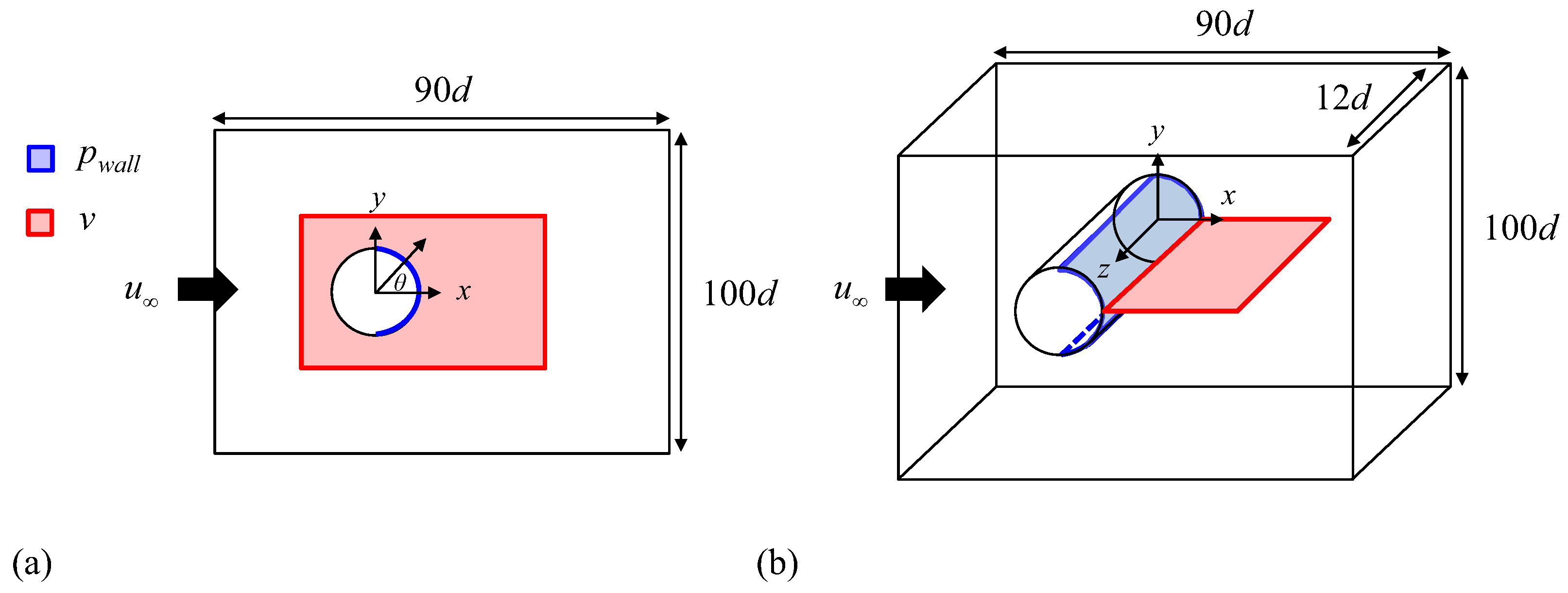
where t is the time, are the Cartesian coordinates, are the corresponding velocity components, and p is the pressure. Here, x, y, and z denote the streamwise, transverse, and spanwise directions, respectively (see Figure 1). To satisfy the no-slip condition on the cylinder surface, we adopt an immersed boundary method by Kim et al. [7]. Owing to the use of the immersed boundary method, Equations (1) and (2) include the mass source/sink term q and the momentum forcing term , respectively. We adopt the fully implicit fractional step method [5,25] to numerically decouple the pressure and velocity in the Navier–Stokes equation using the Crank–Nicolson scheme. The second-order central difference scheme is used for spatial discretizations in each term of Equations (1) and (2). We note that the numerical details described above have been implemented through our own in-house code, and its accuracy has been proven in predicting various complex flow configurations [7,9,26,27].
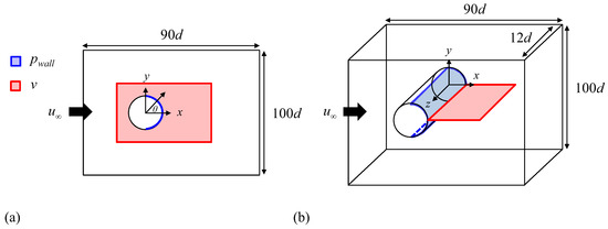
Figure 1.
Computational domains for the numerical simulation of flow over a circular cylinder together with learning dataset domains for machine learning: (a) ; (b) . Blue area: domains for wall pressures as the input variables of neural networks; red area: domains for the transverse velocity prediction as the output variables of neural networks.
Figure 1a,b shows the computational domains for and 300, respectively. The two-dimensional computational domain for is and (see Figure 1a). The computational domain for is three-dimensi
onal with the same x–y domain as that for , and its domain for the spanwise direction is set to be (see Figure 1b). The center axis of a circular cylinder is located at . The numbers of grid points used for numerical simulations are and for and 300, respectively. At the inflow boundary, a Dirichlet boundary condition ( and ) is employed. At the top and bottom boundaries, is given. At the outflow boundary, a convective boundary condition is adopted as , where c is the plane-averaged streamwise velocity on the outflow plane. A periodic boundary condition is applied in the spanwise direction for the three-dimensional computational domain of .
2.2. Dataset
In this study, we aim to predict the near-wake transverse velocity in laminar flow over a circular cylinder by using a neural network with instantaneous wall pressures on the cylinder surface as the input variables. The transverse velocity in the wake of a circular cylinder has been considered a good indicator for the state of Kármán vortex shedding [27,28,29,30,31]. In this regard, one of the motivations for constructing neural networks to predict the transverse velocity is to further integrate them, in future studies, with active feedback control methods such as proportional–integral–derivative (PID) control [27,29], whose control purpose is to mitigate the strength of the Kármán vortex shedding. Figure 1 shows learning dataset domains for neural networks at and 300. As shown in Figure 1a for the two-dimensional flow at , the wall pressures at 44 points on the cylinder surface, ranging from to , constitute the input variables for the learning dataset. Here, represents an angle measured from the base ((,) = (0.5,0)) of the cylinder. The output variables for the learning dataset consist of the transverse velocities v in the ranges of and , encompassing a total of 8192 data points. On the other hand, Figure 1b shows learning dataset domains for input and output variables for the three-dimensional flow at . As shown, the number of input variables for is on the –z plane of the cylinder surface. Here, the locations for and z on the –z plane range from to and from to 12, respectively. The number of output variables for the transverse velocity v is on the finite center plane () of and in the wake of the cylinder. For both and 300, we note that the wall pressures for the input variables are instantaneous ones.
As described in Section 2.1, input and output datasets for training neural networks are obtained from numerical simulations of flow over a circular cylinder at and 300. Consistent with the governing equations in Equations (1) and (2), we adopt dimensionless input and output variables for neural networks, which are non-dimensionalized with the freestream velocity and fluid density. From the numerical simulation of the two-dimensional flow at , we collect 3000 and 1000 instantaneous flow fields as training and testing data, respectively. On the other hand, from the numerical simulation of the three-dimensional flow at , we collect 40,000 and 5000 instantaneous flow fields as training and testing data, respectively. As flow structures become more complex with increasing Reynolds numbers, we use a larger number of instantaneous flow fields for constructing neural networks at compared to that at .
2.3. Details of Neural Networks
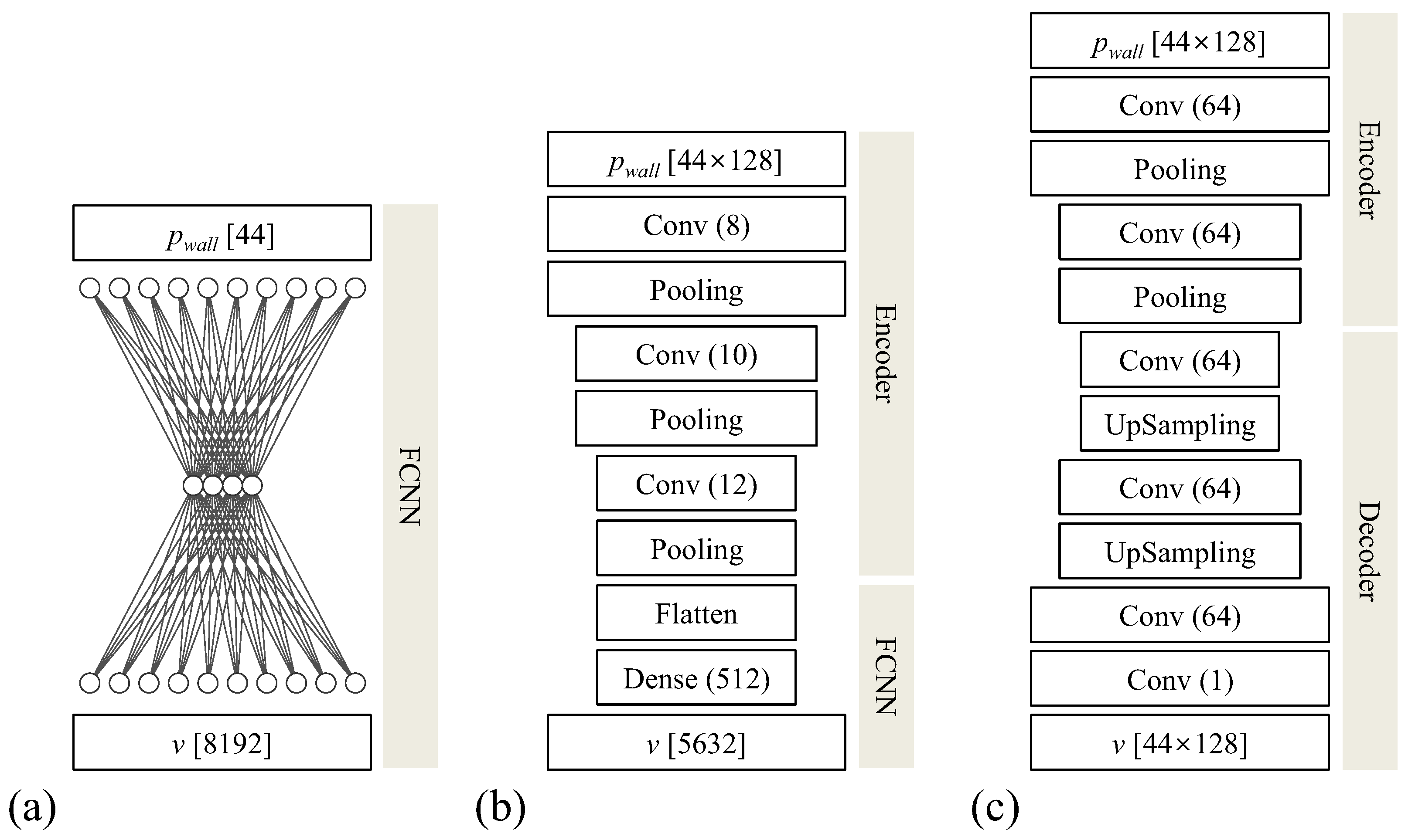
Figure 2 shows schematic diagrams of the present neural networks adopted for and . As shown in Figure 2a, the fully connected neural network for has one hidden layer with four hidden nodes, while the numbers of input () and output (v) variables are 44 and 8192, respectively. In Figure 2b,c, for the case of , we employ two different neural networks of a CNN with an encoder–FCNN structure (CNN-F) and a CNN with an encoder–decoder structure (CNN-D) [32]. In the latter structure, the encoder compresses the input data and encodes them into a latent space, capturing essential features of the input data, while the decoder subsequently generates the output data based on this information [32]. For both encoder–FCNN and encoder–decoder structures employed in CNN as shown in Figure 2b,c, the kernel size of all convolution layers is 5 × 5, the stride is 1, the number of channels is 64, and the number of channels in the last convolution layer is 1. For the activation function for hidden layers, a rectified linear unit (ReLU) is applied [33]. The kernel size and stride of the max pooling and up-sampling layers are and 2, respectively. The up-sampling layers in the neural network as shown in Figure 2c are widely adopted in tasks such as noise reduction for images and image compression and generation [34]. In recent studies adopting CNN with the up-sampling layers [21,22,35], it was found that high-resolution velocity fields in fluid flow could be successfully reconstructed using neural networks with the input of the low-resolution velocity field images. In the present study, we adopt a similar neural network structure with up-sampling layers (Figure 2c) to reconstruct the transverse velocity field in the wake of the cylinder but with the input variables consisting of instantaneous wall pressures on the cylinder surface. For the optimization algorithm during neural network trainings, we use the adaptive moment estimation (Adam) method [36]. Hyperparameters used for trainings are a learning rate of 0.0005, , for the Adam method, and a mini-batch size of 800, which are comparable to those in the study by Jin et al. [24]. In addition, we note that hyperparameters such as the number of channels in Figure 2c were tuned in our preliminary study. The loss function, denoted as , used in the neural network training is defined as follows:
Here, N is the number of training or testing data, and v and represent the transverse velocity obtained from the numerical simulation of flow over a circular cylinder and that predicted by the neural networks as in Figure 2, respectively. Training of neural networks is performed using the open-source software TensorFlow [37].
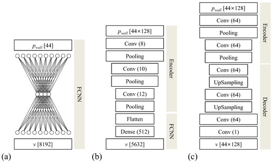
Figure 2.
Schematic diagrams of the present neural networks: (a) fully connected neural networks for ; (b) CNN with an encoder–FCNN structure (CNN-F) for ; (c) CNN with an encoder–decoder structure (CNN-D) for . Here, Conv, Pooling, UpSampling, Flatten, and Dense denote convolutional, max pooling, upsampling, flatten, and dense layers, respectively. is the number of the input/output variables, and is the number of hidden nodes/channels.
3. Results and Discussion
3.1. Simulations of Flows over a Circular Cylinder at = 60 and 300
To acquire training and testing data for constructing neural networks, we first perform numerical simulations of flows over a circular cylinder at and 300. Table 1 shows the flow statistics of laminar flows over a circular cylinder at and 300 obtained from the present numerical simulations, together with those from previous studies. In this table, the mean drag coefficient (), base pressure coefficient (), and Strouhal number () are shown. The base pressure coefficient is the pressure coefficient at the cylinder base (). As shown, for both Reynolds numbers, it is evident that the flow statistics from the present simulations are in good agreements with those of the previous studies, confirming the numerical accuracy of present simulations.

Table 1.
Flow statistics for laminar flows over a circular cylinder at and 300 obtained from the present numerical simulations together with those from previous studies.
3.2. Prediction of Near-Wake Velocity at = 60
In the present study, we use an FCNN with instantaneous wall pressures on the cylinder surface as the input variables to predict the transverse velocity around a circular cylinder at . As illustrated in Figure 1a, 44 locations of wall pressures are used to predict 8192 locations of transverse velocities around the cylinder. This FCNN is constructed by training it with the input and output database of flow fields obtained from the numerical simulation at . The correlation coefficients R between the transverse velocity (v) from the numerical simulation and that () predicted by the FCNN constructed are found to be greater than 0.999 at all locations (Figure 1a) around the cylinder. Here, the correlation coefficient R is defined as follows:
where M is the number of testing data and denotes averaged quantities.
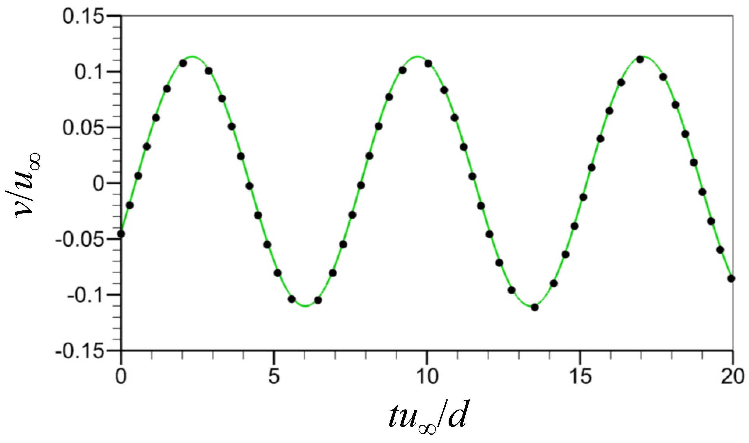
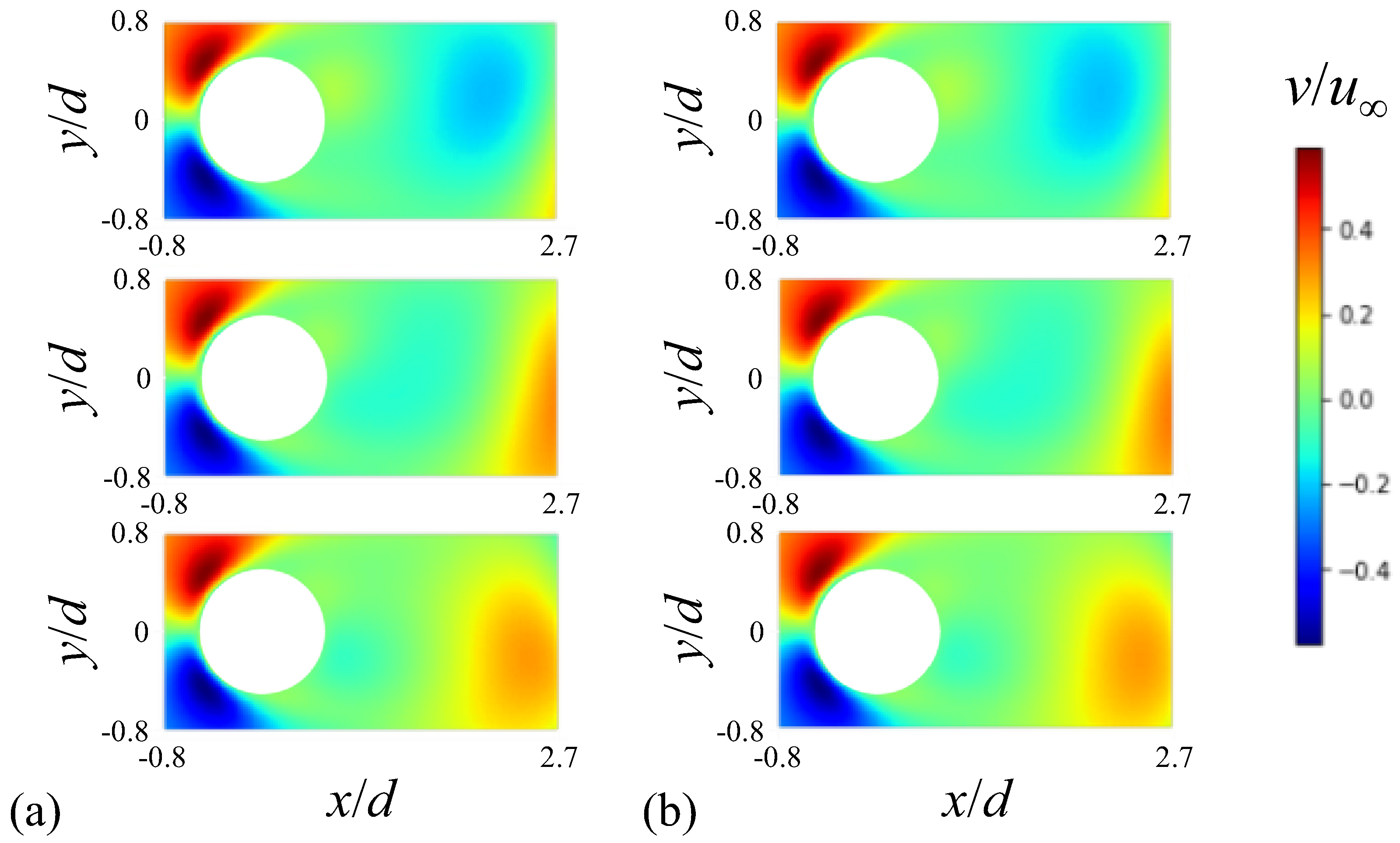
Figure 3 displays the time histories of the transverse velocity at a wake location ( and ) behind the cylinder predicted by the neural network together with that from the numerical simulation at . In the figure, temporal behaviors of the transverse velocity, such as the peak amplitude and temporal periodicity, are well-predicted by the present neural network constructed. Figure 4 shows the contours of the instantaneous transverse velocity predicted by the present FCNN compared with those from the numerical simulation at various temporal instances. As expected from the correlation coefficient of 0.999, the transverse velocity contours agree very well with those from the numerical simulation at all instances.
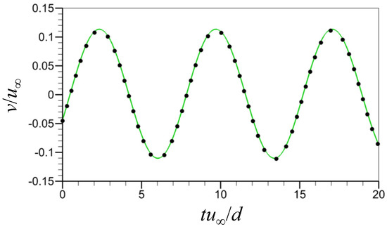
Figure 3.
Time histories of the transverse velocity at and (). ●, from the numerical simulation; green line, predicted by FCNN.

Figure 4.
Contours of the instantaneous transverse velocity at : (a) from the numerical simulation; (b) predicted by FCNN. The three contour plots in (a,b) correspond to temporal instances arbitrarily chosen from the unsteady numerical simulation at .
In the study by Jin et al. [24], they showed that velocity fields in the two-dimensional laminar flow over a circular cylinder could be successfully predicted with neural networks having as their input the pressures on the cylinder surface. In their work, the input variables of the neural network included the pressures at the time together with the pressures at multiple past instances at , and the velocity field at was predicted using these input pressures. On the other hand, our study only employs the instantaneous pressures at the time without past pressure information, resulting in a compact neural network structure. Nevertheless, the prediction quality is comparable to that of Jin et al. [24] at the Reynolds number considered.
3.3. Prediction of Near-Wake Velocity at = 300
In laminar flow over a circular cylinder at , it is well-known that the Kármán vortex shedding maintains its two-dimensionality without spanwise variations in its vortical structure [1,41]. Thus, we considered two-dimensional flow at in Section 3.2. However, the Kármán vortex shedding behind a circular cylinder becomes three-dimensional for , where spanwise variations in vortical structures are observed owing to the occurrences of vortex loops and streamwise vortices [1,41]. Therefore, predictions of the wake flow field over a circular cylinder at would be a more difficult task than those at . In the present study, to predict the transverse velocity on the centerplane in the near-wake behind the cylinder at , we construct two different neural network structures (CNN-F and CNN-D) as described in Figure 2b,c. We note that a neural network similar to CNN-F was used in the study of Jin et al. [24].
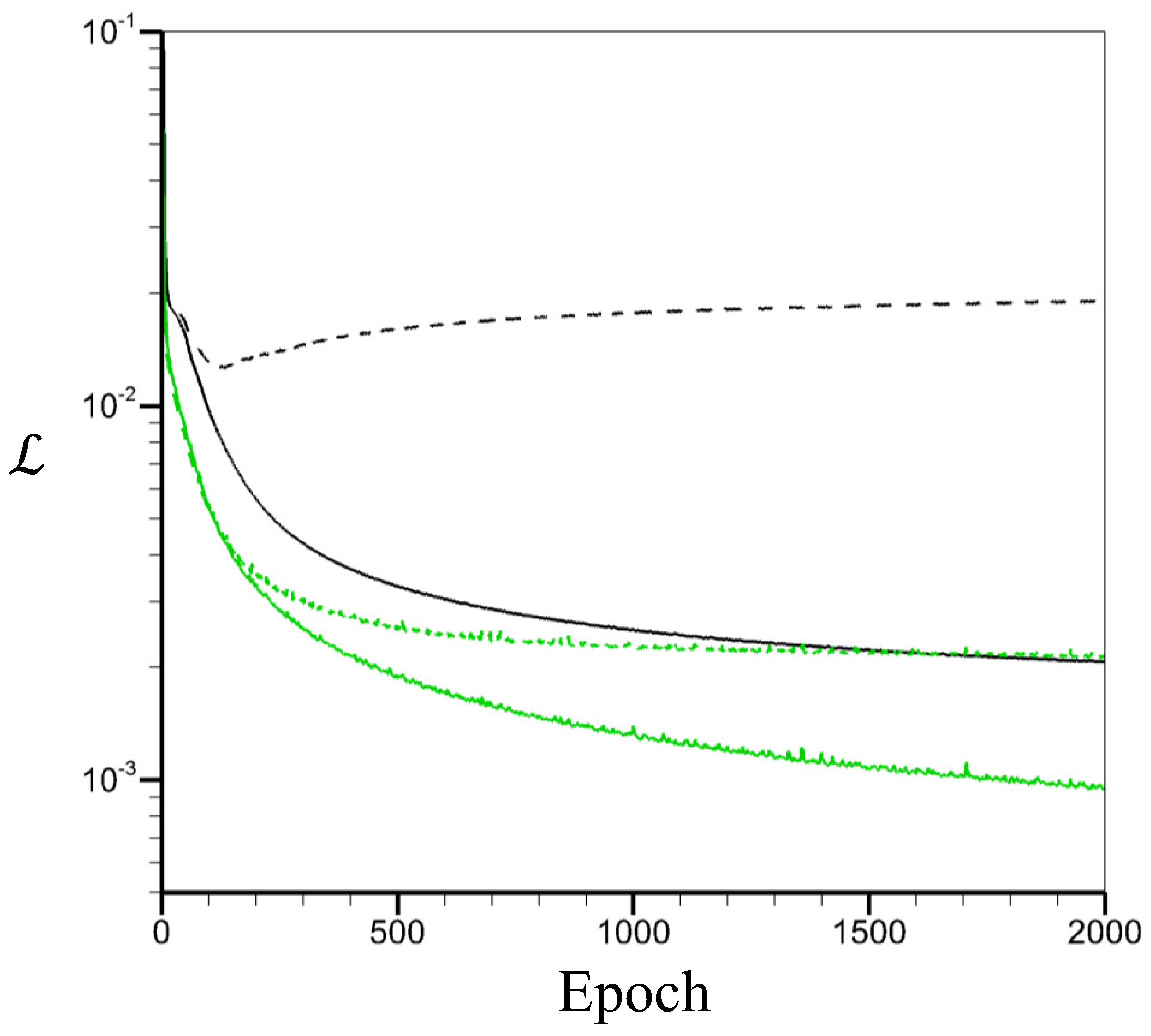
Figure 5 shows loss functions versus the number of epochs for the training of both CNN-D and CNN-F structures at . As shown, CNN-D exhibits lower values of loss function than CNN-F as the number of epochs increases, suggesting that CNN-D has better prediction accuracy for the hyperparameters and dataset considered in this study. Notably, during the learning process of CNN-F, the value of loss function for testing data increases after 100 epochs, which suggests that a mild overfitting occurs for CNN-F. We suspect that this overfitting occurs because the number of instantaneous flow fields is insufficient for the proper training of CNN-F. On the other hand, CNN-D does not exhibit an overfitting behavior. We believe that this could be attributed to the fact that the decoder structure of CNN-D has fewer parameters in hidden layers than the FCNN structure of CNN-F, making it less vulnerable to overfitting when dealing with a smaller dataset.
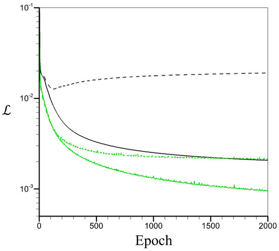
Figure 5.
Loss functions versus the number of epochs for the training of neural networks at : black line, CNN-F; green line, CNN-D; solid line, training loss; dashed line, testing loss.
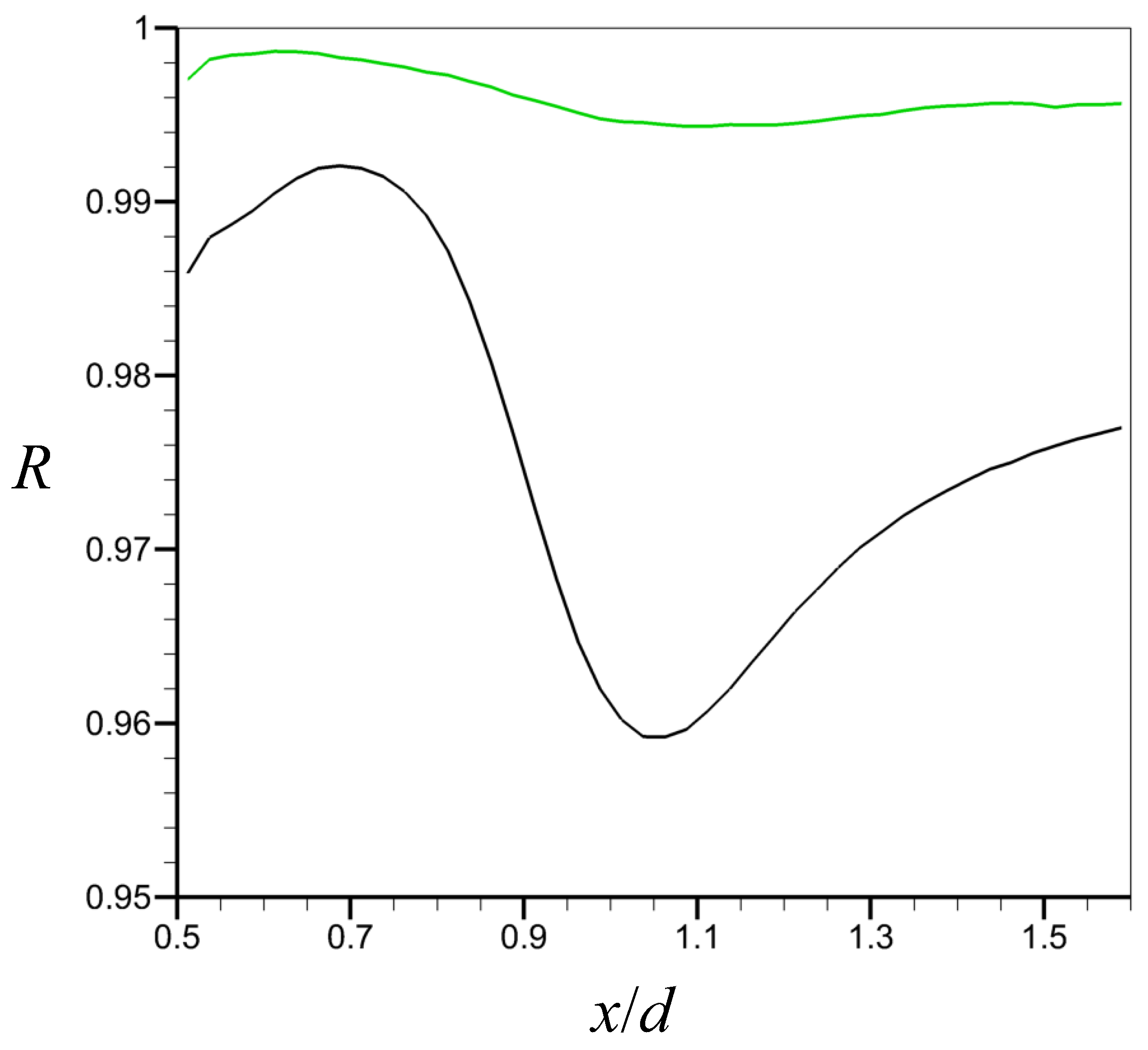
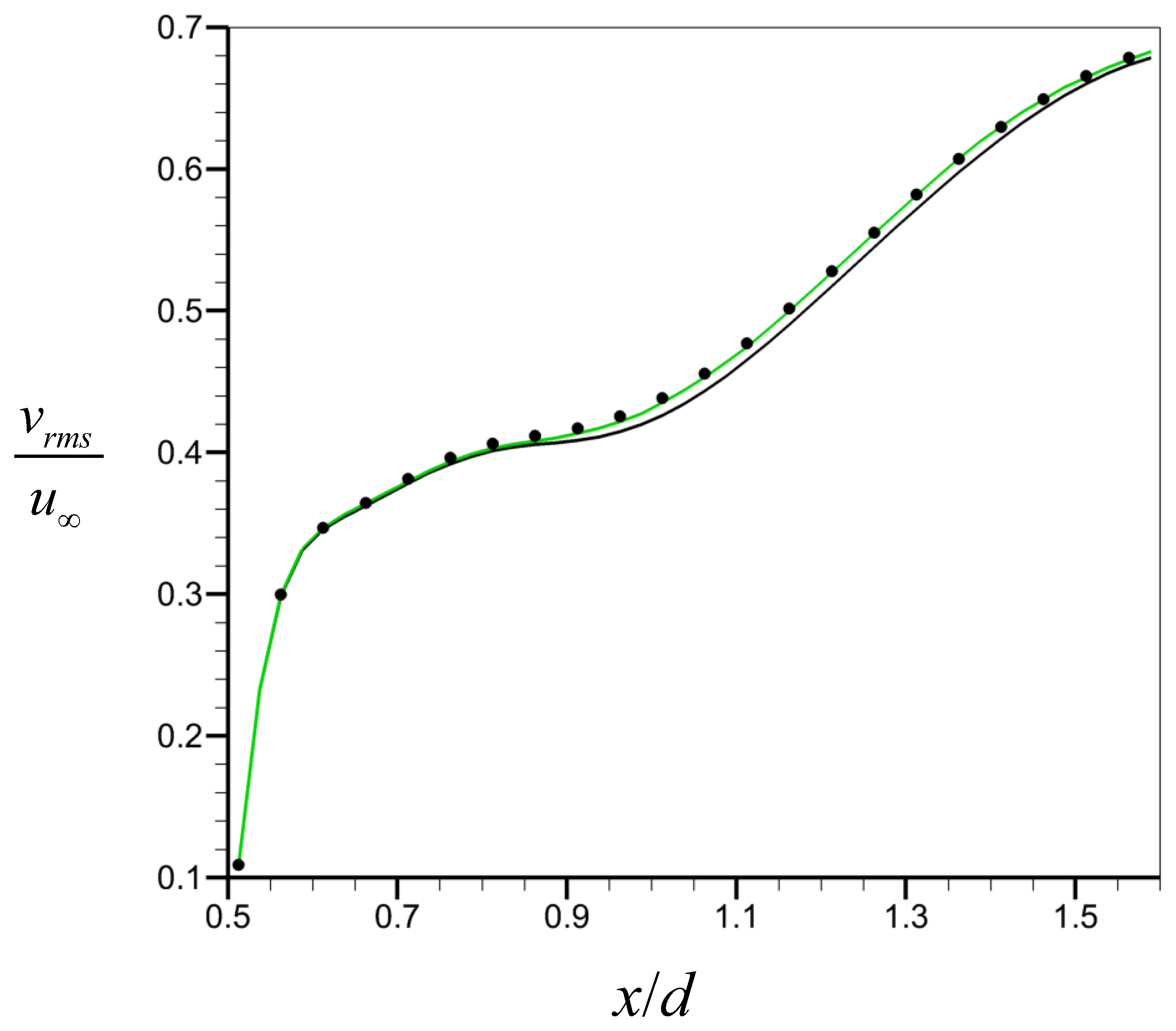
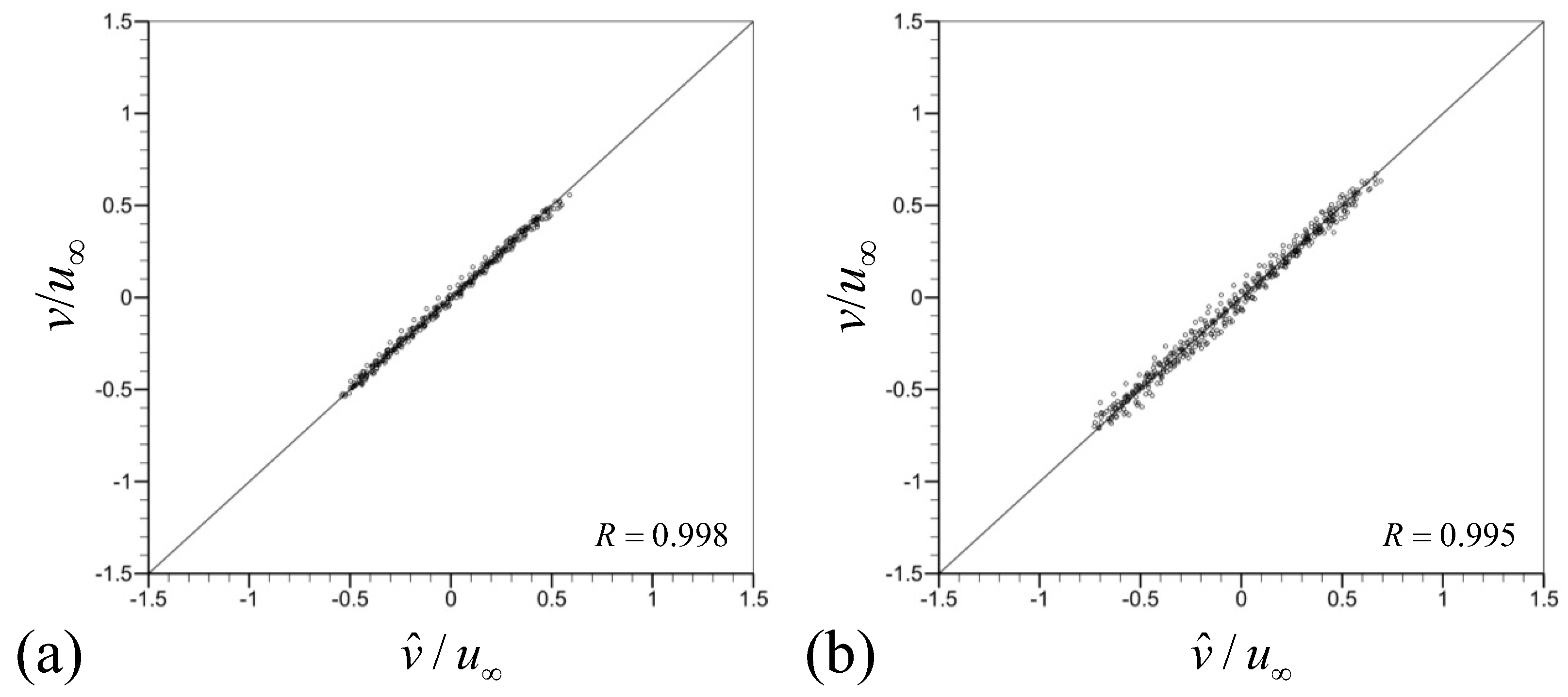
Figure 6 shows the correlation function R according to the streamwise location () at , where R is obtained by Equation (4). Here, owing to the statistical homogeneity in the spanwise direction, we conduct an averaging of R in the spanwise direction. As shown, the prediction performance of CNN-D is superior to that of CNN-F at all streamwise locations. Compared to CNN-F with an average of , the prediction using CNN-D yields an average of with variations of depending on x. This superiority of CNN-D over CNN-F is also evident in the root mean square (rms) of transverse velocity on the centerplane of the wake presented in Figure 7. The rms of transverse velocity from CNN-D agrees very well with that from the numerical simulation, while that from CNN-F shows a slight deviation. Figure 8 shows the scatter plots of from the numerical simulation and predicted by CNN-D at two different streamwise locations ( and ). For both locations, the transverse velocity predicted by CNN-D shows a good prediction performance, supporting the results of Figure 5, Figure 6 and Figure 7.
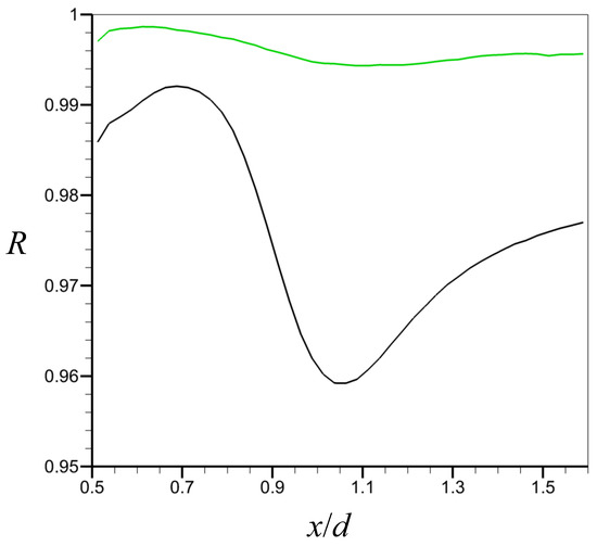
Figure 6.
Correlation function R on the centerplane of the wake at . Black line, R from CNN-F; green line, R from CNN-D.
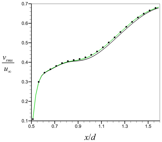
Figure 7.
Root mean square of transverse velocity on the centerplane of the wake at . ●, from the numerical simulation; black line, predicted by CNN-F; green line, predicted by CNN-D.
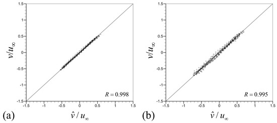
Figure 8.
Scatter plots of from the numerical simulation and predicted by CNN-D at . (a) (); (b) ().
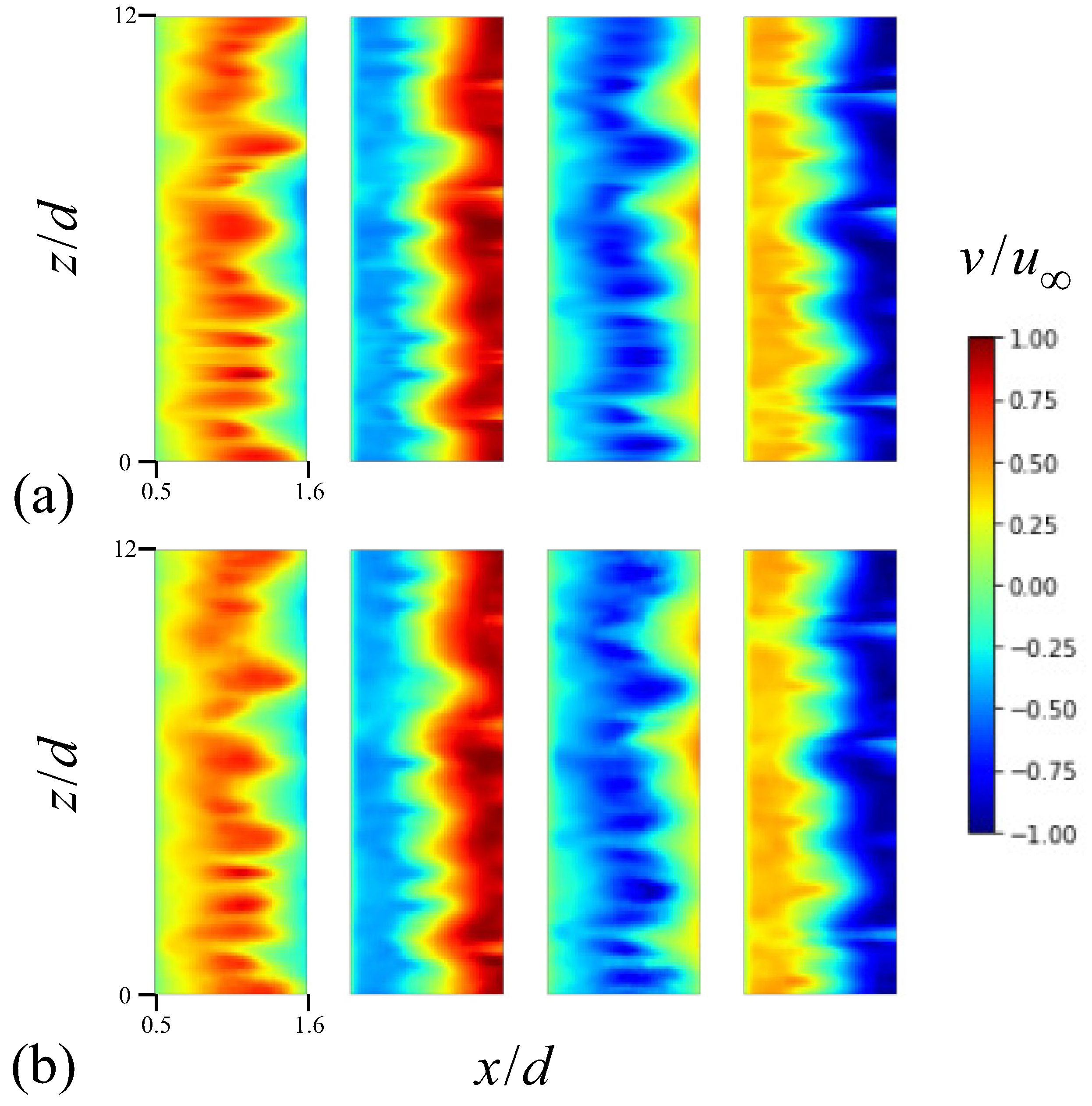
Figure 9 presents the time histories of the transverse velocity at the point of and in the wake for . The velocity from CNN-D accurately follows the temporal behaviors of the numerical simulation, while that from CNN-F becomes less accurate in the vicinity of the peak locations of the velocity. Figure 10 displays the contours of the instantaneous transverse velocity on the x–z plane of (centerplane) predicted by CNN-D, together with those from the numerical simulation at four different temporal instances. From Figure 10a, the transverse velocity from the numerical simulation displays significant spanwise variations that change over time. These variations in Figure 10a compare very well with those predicted by the present neural network of CNN-D, as demonstrated in Figure 10b.
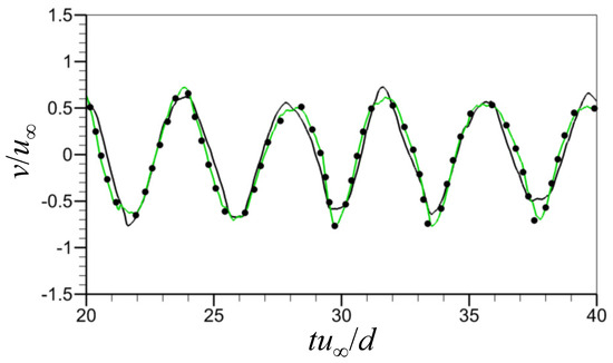
Figure 9.
Time histories of the transverse velocity at the point of and in the wake for . ●, from the numerical simulation; black line, predicted by CNN-F (); green line, predicted by CNN-D ().

Figure 10.
Contours of the instantaneous transverse velocity on the centerplane () at different temporal instances for : (a) from the numerical simulation; (b) predicted by CNN-D. Here, the four contour plots in (a,b) correspond to temporal instances arbitrarily chosen from the unsteady numerical simulation at .
4. Conclusions
In the present study, to predict the transverse velocity field in the near-wake of laminar flow over a circular cylinder at the Reynolds numbers of 60 and 300, we constructed neural networks with instantaneous wall pressures on the cylinder surface as the input variables. For the two-dimensional unsteady flow at , a fully connected neural network was considered. On the other hand, for the three-dimensional unsteady flow at having spanwise variations, we employed two different convolutional neural networks of CNN-F and CNN-D. Numerical simulations were carried out for both Reynolds numbers to obtain instantaneous flow fields, from which the input and output datasets were generated for training these neural networks. At the Reynolds numbers considered, the neural networks constructed accurately predicted the transverse velocity fields in the near-wake over the cylinder using the information of instantaneous wall pressures as the input variables. In addition, at , it was observed that CNN-D showed a better prediction ability than CNN-F.
The neural networks in this study were trained at a specific Reynolds number. Consequently, their performance at predicting other Reynolds numbers may not be as reliable. To improve the prediction performance for a wider range of Reynolds numbers, one could consider training the networks using flow fields from various Reynolds numbers. In addition, flow structures such as flow separation, shear layer, and wake are commonly observed in the flow over a cylinder across different Reynolds numbers. Designing neural networks to consider these features could therefore be a promising approach for future studies.
The transverse velocity in the near-wake of the cylinder is a useful information indicating the status of the Kármán vortex shedding. Thus, various feedback controls applied to flow over a circular cylinder measure the transverse velocity in the wake as sensors and aim to reduce its amplitude to weaken the strength of the Kármán vortex shedding [27,28,29,30,31]. However, it would not be practical to measure the transverse velocity in the wake in real applications of these control methods. Therefore, we believe that incorporating the present neural networks with feedback control methods would be an effective control strategy to improve its practical applicability because this approach does not need to measure the velocity and only measures the wall pressures as a sensor of feedback controller [27].
Author Contributions
Conceptualization, methodology, investigation: J.Y. and J.L.; validation, formal analysis, writing—original draft preparation, visualization: J.Y. and J.L.; writing—review and editing, supervision, project administration, funding acquisition: J.L. All authors have read and agreed to the published version of the manuscript.
Funding
This research was supported by Basic Science Research Program through the National Research Foundation of Korea (NRF) funded by the Ministry of Education (2016R1D1A1B03932120). Additionally, this work was supported by Korea Ministry of Environment (MOE) as “Chemical Accident Advancement Project” (No. 2022003620005/1485018894).
Data Availability Statement
The data presented in this study are available from the corresponding author upon reasonable request.
Conflicts of Interest
The authors declare no conflict of interest.
Nomenclature
| x | Streamwise direction |
| y | Transverse direction |
| z | Spanwise direction |
| Angle from the cylinder base | |
| t | Time |
| u | Streamwise velocity |
| v | Transverse velocity |
| w | Spanwise velocity |
| p | Pressure |
| d | Cylinder diameter |
| Free stream velocity | |
| Kinematic viscosity | |
| Reynolds number | |
| Drag coefficient | |
| Pressure coefficient at the cylinder base | |
| Strouhal number | |
| Wall pressure on a circular cylinder | |
| Transverse velocity predicted by neural network | |
| Loss function | |
| q | Mass source/sink |
| f | Momentum forcing |
| N | Number of training or testing data |
| R | Correlation coefficient |
References
- Williamson, C. Vortex dynamics in the cylinder wake. Annu. Rev. Fluid Mech. 1996, 28, 477–512. [Google Scholar] [CrossRef]
- Westerweel, J.; Elsinga, G.E.; Adrian, R.J. Particle image velocimetry for complex and turbulent flows. Annu. Rev. Fluid Mech. 2013, 45, 409–436. [Google Scholar] [CrossRef]
- Soria, J. An investigation of the near wake of a circular cylinder using a video-based digital cross-correlation particle image velocimetry technique. Exp. Therm. Fluid Sci. 1996, 12, 221–233. [Google Scholar] [CrossRef]
- Wu, Z.; Choi, H. Modification of flow behind a circular cylinder by steady and time-periodic blowing. Phys. Fluids 2021, 33, 115126. [Google Scholar] [CrossRef]
- Kim, J.; Moin, P. Application of a fractional-step method to incompressible Navier–Stokes equations. J. Comput. Phys. 1985, 59, 308–323. [Google Scholar] [CrossRef]
- Moin, P.; Mahesh, K. Direct numerical simulation: A tool in turbulence research. Annu. Rev. Fluid Mech. 1998, 30, 539–578. [Google Scholar] [CrossRef]
- Kim, J.; Kim, D.; Choi, H. An immersed-boundary finite-volume method for simulations of flow in complex geometries. J. Comput. Phys. 2001, 171, 132–150. [Google Scholar] [CrossRef]
- Vreman, A. An eddy-viscosity subgrid-scale model for turbulent shear flow: Algebraic theory and applications. Phys. Fluids 2004, 16, 3670–3681. [Google Scholar] [CrossRef]
- Park, N.; Lee, S.; Lee, J.; Choi, H. A dynamic subgrid-scale eddy viscosity model with a global model coefficient. Phys. Fluids 2006, 18, 125109. [Google Scholar] [CrossRef]
- Lee, J.; Choi, H.; Park, N. Dynamic global model for large eddy simulation of transient flow. Phys. Fluids 2010, 22, 075106. [Google Scholar] [CrossRef]
- Ling, J.; Kurzawski, A.; Templeton, J. Reynolds averaged turbulence modelling using deep neural networks with embedded invariance. J. Fluid Mech. 2016, 807, 155–166. [Google Scholar] [CrossRef]
- Maulik, R.; San, O. A neural network approach for the blind deconvolution of turbulent flows. J. Fluid Mech. 2017, 831, 151–181. [Google Scholar] [CrossRef]
- Stolz, S.; Adams, N.A. An approximate deconvolution procedure for large-eddy simulation. Phys. Fluids 1999, 11, 1699–1701. [Google Scholar] [CrossRef]
- Park, J.; Choi, H. Toward neural-network-based large eddy simulation: Application to turbulent channel flow. J. Fluid Mech. 2021, 914, A16. [Google Scholar] [CrossRef]
- Gamahara, M.; Hattori, Y. Searching for turbulence models by artificial neural network. Phys. Rev. Fluids 2017, 2, 054604. [Google Scholar] [CrossRef]
- Wang, Z.; Luo, K.; Li, D.; Tan, J.; Fan, J. Investigations of data-driven closure for subgrid-scale stress in large-eddy simulation. Phys. Fluids 2018, 30, 125101. [Google Scholar] [CrossRef]
- Sarghini, F.; De Felice, G.; Santini, S. Neural networks based subgrid scale modeling in large eddy simulations. Comput. Fluids 2003, 32, 97–108. [Google Scholar] [CrossRef]
- Germano, M.; Piomelli, U.; Moin, P.; Cabot, W.H. A dynamic subgrid-scale eddy viscosity model. Phys. Fluids A Fluid Dyn. 1991, 3, 1760–1765. [Google Scholar] [CrossRef]
- Lilly, D.K. A proposed modification of the Germano subgrid-scale closure method. Phys. Fluids A Fluid Dyn. 1992, 4, 633–635. [Google Scholar] [CrossRef]
- Brunton, S.L.; Noack, B.R.; Koumoutsakos, P. Machine learning for fluid mechanics. Annu. Rev. Fluid Mech. 2020, 52, 477–508. [Google Scholar] [CrossRef]
- Fukami, K.; Fukagata, K.; Taira, K. Super-resolution reconstruction of turbulent flows with machine learning. J. Fluid Mech. 2019, 870, 106–120. [Google Scholar] [CrossRef]
- Fukami, K.; Fukagata, K.; Taira, K. Machine-learning-based spatio-temporal super resolution reconstruction of turbulent flows. J. Fluid Mech. 2021, 909, A9. [Google Scholar] [CrossRef]
- Lee, S.; You, D. Data-driven prediction of unsteady flow over a circular cylinder using deep learning. J. Fluid Mech. 2019, 879, 217–254. [Google Scholar] [CrossRef]
- Jin, X.; Cheng, P.; Chen, W.L.; Li, H. Prediction model of velocity field around circular cylinder over various Reynolds numbers by fusion convolutional neural networks based on pressure on the cylinder. Phys. Fluids 2018, 30, 047105. [Google Scholar] [CrossRef]
- Kim, K.; Baek, S.J.; Sung, H.J. An implicit velocity decoupling procedure for the incompressible Navier–Stokes equations. Int. J. Numer. Methods Fluids 2002, 38, 125–138. [Google Scholar] [CrossRef]
- Kim, W.; Lee, J.; Choi, H. Flow around a helically twisted elliptic cylinder. Phys. Fluids 2016, 28, 053602. [Google Scholar] [CrossRef]
- Yun, J.; Lee, J. Active proportional feedback control of turbulent flow over a circular cylinder with averaged velocity sensor. Phys. Fluids 2022, 34, 095133. [Google Scholar] [CrossRef]
- Park, D.; Ladd, D.; Hendricks, E. Feedback control of von Kármán vortex shedding behind a circular cylinder at low Reynolds numbers. Phys. Fluids 1994, 6, 2390–2405. [Google Scholar] [CrossRef]
- Son, D.; Jeon, S.; Choi, H. A proportional–integral–differential control of flow over a circular cylinder. Philos. Trans. R. Soc. A 2011, 369, 1540–1555. [Google Scholar] [CrossRef]
- Son, D.; Choi, H. Iterative feedback tuning of the proportional-integral-differential control of flow over a circular cylinder. IEEE Trans. Control. Syst. Technol. 2018, 27, 1385–1396. [Google Scholar] [CrossRef]
- Jiang, H.; Cheng, L. Transition to the secondary vortex street in the wake of a circular cylinder. J. Fluid Mech. 2019, 867, 691–722. [Google Scholar] [CrossRef]
- Baldi, P. Autoencoders, unsupervised learning, and deep architectures. In Proceedings of the ICML Workshop on Unsupervised and Transfer Learning, Bellevue, WA, USA, 2 July 2011; pp. 37–49. [Google Scholar]
- Nair, V.; Hinton, G.E. Rectified linear units improve restricted boltzmann machines. In Proceedings of the 27th International Conference on Machine Learning (ICML-10), Haifa, Israel, 21–24 June 2010; pp. 807–814. [Google Scholar]
- Bank, D.; Koenigstein, N.; Giryes, R. Autoencoders. arXiv 2020, arXiv:2003.05991. [Google Scholar]
- Liu, B.; Tang, J.; Huang, H.; Lu, X.Y. Deep learning methods for super-resolution reconstruction of turbulent flows. Phys. Fluids 2020, 32, 025105. [Google Scholar] [CrossRef]
- Kingma, D.P.; Ba, J. Adam: A method for stochastic optimization. arXiv 2014, arXiv:1412.6980. [Google Scholar]
- Abadi, M.; Agarwal, A.; Barham, P.; Brevdo, E.; Chen, Z.; Citro, C.; Corrado, G.S.; Davis, A.; Dean, J.; Devin, M.; et al. Tensorflow: Large-scale machine learning on heterogeneous distributed systems. arXiv 2016, arXiv:1603.04467. [Google Scholar]
- Park, J.; Kwon, K.; Choi, H. Numerical solutions of flow past a circular cylinder at Reynolds numbers up to 160. KSME Int. J. 1998, 12, 1200–1205. [Google Scholar] [CrossRef]
- Kravchenko, A.G.; Moin, P.; Shariff, K. B-spline method and zonal grids for simulations of complex turbulent flows. J. Comput. Phys. 1999, 151, 757–789. [Google Scholar] [CrossRef]
- Jiang, H.; Cheng, L.; Draper, S.; An, H.; Tong, F. Three-dimensional direct numerical simulation of wake transitions of a circular cylinder. J. Fluid Mech. 2016, 801, 353–391. [Google Scholar] [CrossRef]
- Williamson, C. The existence of two stages in the transition to three-dimensionality of a cylinder wake. Phys. Fluids 1988, 31, 3165–3168. [Google Scholar] [CrossRef]
Disclaimer/Publisher’s Note: The statements, opinions and data contained in all publications are solely those of the individual author(s) and contributor(s) and not of MDPI and/or the editor(s). MDPI and/or the editor(s) disclaim responsibility for any injury to people or property resulting from any ideas, methods, instructions or products referred to in the content. |
© 2023 by the authors. Licensee MDPI, Basel, Switzerland. This article is an open access article distributed under the terms and conditions of the Creative Commons Attribution (CC BY) license (https://creativecommons.org/licenses/by/4.0/).

