Effect of Cohesive Properties on Low-Velocity Impact Simulations of Woven Composite Shells

Abstract

The effect of the interface stiffness and interface strength on the low-velocity impact response of woven-fabric semicylindrical composite shells is studied using finite element (FE) models generated with continuum shell elements and cohesive surfaces. The intralaminar damage is accounted for using the constitutive model provided within the ABAQUS software, while the interlaminar is addressed utilising cohesive surfaces. The results show that the interface stiffness has a negligible effect on the force and energy histories for values between 10${}^1$ N/mm${}^3$ and 2.43 × 10${}^6$ N/mm${}^3$. However, it has a significant impact on the delamination predictions. It is observed that only the normal interface strength affects the maximum impact force and the delamination predictions. Increasing its value from 15 MPa to 30 MPa resulted in an 8% growth in the maximum force, and a substantial reduction in the delaminated area. The obtained results serve as guidelines for the accurate and efficient computation of delamination. The successful validation of the FE models establishes a solid foundation for further numerical investigations and offers the potential to significantly reduce the time and expenses associated with experimental testing.

1. Introduction

Low-velocity impact tests are commonly employed for assessing the damage resistance and tolerance of fibre-reinforced composite structures. The extensive research in this area focuses on experimental analysis, aiming to comprehend the intricate progressive degradation of the material, considering inter-related failure mechanisms [1,2].

The intrinsic characteristics of the structure and of the impactor, and the prevailing environmental conditions collectively influence the structural response to low-velocity impact events. Visual inspection of the damaged area, measurement of dent depth, and a nondestructive evaluation, such as C-Scan, may be used to assess the damage extension in a structure that has experienced low-velocity impact(s) [3].

Typically, matrix cracking is the initial failure observed at the onset of the impact force. Subsequently, delaminations are induced by the matrix cracking and propagate further as the applied force continues to increase. A substantial decrease in force can frequently be used to detect the emergence of notable delaminations [4]. Depending on the amount of impact energy, there may be noticeable fibre breakage after the delamination has grown. Due to the flexibility of the matrix and the disorganisation of the broken fibres, persistent indentation may appear after the impact [5].

Understanding the phenomenon of impact damage in laminated composite structures presents a significant analytical challenge due to its intricate and complex nature. The numerical models built using the finite element (FE) method, on the other hand, are a powerful tool for predicting physical processes. Many different impact configurations and structures can be studied using FE models, especially in situations when experimental testing would be prohibitively expensive or complex [6,7,8,9]. The computing requirements increase as the model’s complexity increases. Hence, there is a need to dedicate efforts towards developing time-efficient FE models.

Simulating low-velocity impact tests on composite structures poses a challenging problem due to the occurrence of contact and progressive degradation of the material. Consequently, it is crucial to accurately model the interlaminar and intralaminar failure mechanisms within an FE analysis. Additionally, defining several important parameters that can impact the precision of numerical predictions, such as material properties, element types, FE mesh discretization, assembly of the parts, and imposed boundary conditions, becomes imperative [10].

There is a scarcity of numerical studies focusing on the impact dynamics of cylindrical composite shells. Among the notable studies, Kim et al. [11] conducted research that revealed a relationship between the curvature of composite shell and the contact force. They observed an increase in contact force with a higher shell curvature, accompanied by a decrease in deflection and the contact duration. Furthermore, they found that the velocity of the impactor had a more significant influence on the contact force compared to the mass of the impactor. Another noteworthy study by Choi [12] demonstrated a similar contact force and deflection. Zhao and Cho investigated the onset and evolution of impact damage in composite shells [13], while Kistler and Wass established scaling relationships between impact energy, momentum, mass, and velocity [14]. In their investigation, Kumar et al. [15] employed an FE analysis to examine the impact behaviour of cylindrical composite shells.

This paper aims to study the effect of the cohesive properties on the numerical predictions of low-velocity impact events on woven-fabric composite shells. This work is based on the FE modelling strategy presented in [16] and the experimental testing performed in [2]. The ABAQUS/Explicit [17] VUMAT subroutine specifically designed for fabric-reinforced composites was used to capture the intralaminar damage [18]. Simultaneously, a surface-based cohesive model (S-BCM) was implemented to account for the interlaminar damage.

The document is structured as follows: Section 2 provides a comprehensive overview of the FE modelling approach employed, encompassing the description of intra- and interlaminar damage models, FE mesh discretisation, and boundary conditions and contact definitions. In Section 3, the accuracy of the numerical predictions regarding delamination, force, and energy histories is thoroughly assessed by comparing the results with experimental evidence, while considering the influence of interface stiffness and strength. Finally, Section 4 presents the key findings and main conclusions derived from this study.

2. Finite Element Models

In this section, the approaches employed for generating the FE models of semicylindrical composite shells are presented. It encompasses the constitutive models utilised to simulate both intralaminar and interlaminar material impact induced damage on the semicylindrical composite shells. Additionally, it provides a concise description of the element types and sizes, the boundary conditions, and the contact definitions imposed to replicate the experimental setup.

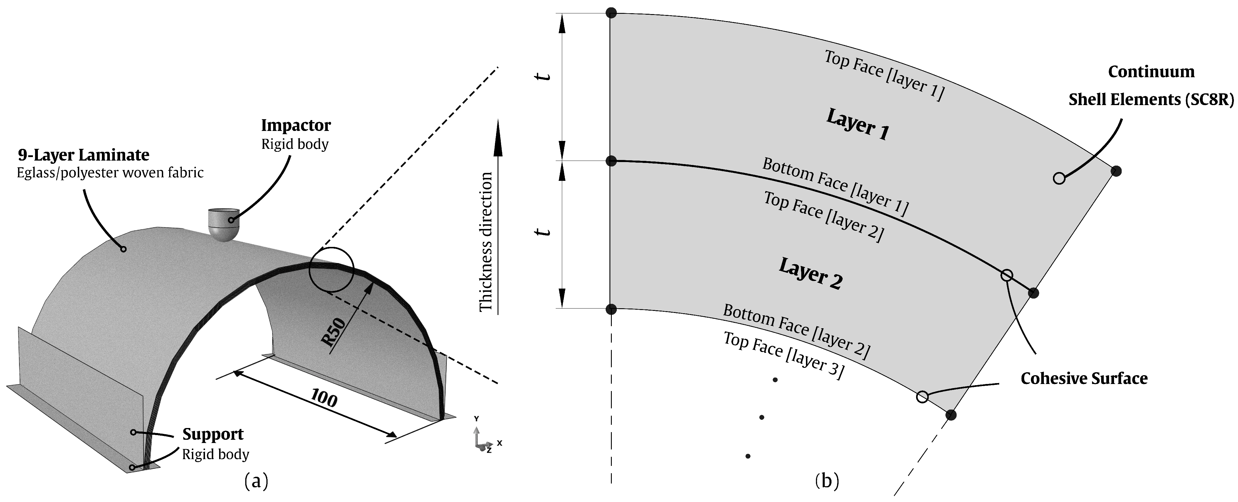
2.1. Finite Element Modelling Approach

Nine plain weaves of glass fibres at 0 and 90 degrees with 98 ± 4% g/m${}^2$ in each direction were combined with an AROPOL FS 1962 polyester resin and a MEKP-50 hardener to produce the semicylindrical composite shells shown in Figure 1. This figure also shows a schematic representation of the shell layup generated with continuum shell elements. These elements provide an efficient and accurate way to simulate the behaviour of shell structures under various loading conditions, making them suitable to study composite shells structures. Moreover, they are computationally efficient when compared to solid elements.

To model the interlaminar behaviour, cohesive surfaces were added to the interfaces of adjacent layers. The cohesive behaviour was applied to the nodes that were initially in contact, meaning that any new contact that occurred during the analysis did not experience cohesive constrain forces. The cohesive surfaces are directly related to the shell elements and share the same FE mesh size. In this way, they provide a simple way to model the interlaminar connection in negligible small interface thicknesses. The use of this strategy for modelling the interlaminar damage implies that the S-BCM must be defined as a surface interaction property and not as a material property. The main advantage of this approach is the quick and easy modelling of the cohesive connection. Moreover, it often allows for higher stable time increments than cohesive elements and does not add any mass to the FE model.

The simulations were conducted using a semiautomatic mass-scaling technique that was uniformly applied to the entire FE model. A target time increment of 1 × 10${}^{-7}$ was employed during the simulations. This approach resulted in an overall mass increase of 1.8%. However, it also provided a notable benefit in terms of computational efficiency, reducing the computational cost of the solution by approximately 50%.

2.2. Intralaminar Damage Modelling

To capture the progression of damage at the intralaminar level, a constitutive model specifically designed for fabric-reinforced composites, was used in ABAQUS/Explicit [17]. This constitutive model, initially developed by Johnson et al. [19] and based on the work of Ladeveze and Ledantec [20], offers comprehensive capabilities for capturing the intralaminar damage phenomena. It can be seamlessly integrated into the analysis workflow as a VUMAT user subroutine, with the user-defined material identified by the text “ABQ_PLY_FABRIC” [18]. This integration enables effective modelling and simulation of the intralaminar damage process in fabric-reinforced composites. In this damage model, each woven fabric-reinforced layer is modelled as a homogeneous orthotropic elastic material with the capability of sustaining progressive stiffness degradation due to fibre failure and matrix cracking, and plastic deformation under shear loading [16,18].

Notice that in the absence of specific experimental data for the tested material, reference values from similar studies/materials were employed as a starting point. However, recognising the need for a more refined and comprehensive analysis, a parametric study was conducted to thoroughly investigate and evaluate the influence of fracture toughness on the numerical-experimental correlation.

The intralaminar damage model utilised in this study adopts the maximum stress failure criterion to determine the initiation of damage in the fibres. Additionally, a damage evolution model based on fracture energies was employed to govern the progressive reduction in stiffness. To describe the mechanical behaviour of the degraded orthotropic material, the Hooke’s law was applied, and its expression is as follows:

$$\epsilon =\left[\begin{array}{ccc}\frac{S_1}{\left(1-d_1\right)}& S_{12}& 0\\ S_{21}& \frac{S_2}{\left(1-d_2\right)}& 0\\ 0& 0& \frac{S_6}{\left(1-d_{12}\right)}\end{array}\right]\sigma$$

(1)

where $S_{ij}$ represents the components of the compliance matrix for the undamaged orthotropic material. The nominal Cauchy stress tensor is denoted as $\sigma$, while $\epsilon$ represents the elastic strain tensor. The damage coefficients, $d_1$, $d_2$, and $d_{12}$, have specific associations: $d_1$ and $d_2$ relate to fibre fracture along directions 1 and 2, respectively, whereas $d_{12}$ corresponds to matrix microcracking caused by shear deformation.

The elastic domain, at any given time, is calculated based on the damage activation functions, $F_{\alpha }$, expressed as:

$$F_{\alpha }=\frac{{\tilde{\sigma }}_{\alpha }}{X_{\alpha }}-r_{\alpha }\le 0\mathrm{with}\alpha =1\pm ,2\pm ,12$$

(2)

where ${\tilde{\sigma }}_{\alpha }$ and $X_{\alpha }$ represent the effective stresses and strengths, respectively, and $r_{\alpha }$ denotes the damage thresholds, initially set to 1. Once the damage onset is reached, indicated by $\frac{{\tilde{\sigma }}_{\alpha }}{X_{\alpha }}=1$, the evolution of the damage coefficients $d_1$ and $d_2$ (associated with tensile and compressive loading) is determined using Equations (3) and (4). Similarly, the damage coefficient $d_{12}$ (related to shear loading) is obtained from Equation (5).

$$d_{1,2}=1-\frac{1}{r_{1,2}}{e}^{-A_{1,2}\left(r_{1,2}-1\right)}$$

(3)

$$A_{1,2}=\frac{2g_0^{1,2}{L}_{ch}}{G_f^{1,2}-g_0^{1,2}{L}_{ch}}\mathrm{with}{g}_0^{1,2}=\frac{X_{1,2}^2}{2E_{1,2}}$$

(4)

$$d_{12}=min\left[{\alpha }_{12}ln\left(r_{12}\right),d_{12}^{max}\right]$$

(5)

where $r_{1,2}$ and $r_{12}$ represent the damage thresholds for tensile/compressive and shear loading, respectively, $G_f^{1,2}$ refers to the fracture energies per unit area, $g_0^{1,2}$ corresponds to the elastic energy density at the damage onset, and $L_{ch}$ represents the characteristic length of the element. The shear damage parameter ${\alpha }_{12}$ is determined through a calibration procedure outlined in [18].

At the intralaminar level, the shear damage response is driven by the nonlinear behaviour of the matrix due to matrix microcracking. This response involves both stiffness loss and plasticity. The VUMAT subroutine employs yield and hardening functions, as shown in Equations (6) and (7), to define the plasticity response of the matrix:

$$F_{pl}=\left|{\tilde{\sigma }}_{12}\right|-{\tilde{\sigma }}_0({\overline{\epsilon }}^{pl})\le 0$$

(6)

$${\tilde{\sigma }}_0({\overline{\epsilon }}^{pl})={\tilde{\sigma }}_{y0}+C{({\overline{\epsilon }}^{pl})}^p$$

(7)

where ${\tilde{\sigma }}_{12}$ represents the effective shear stress, ${\tilde{\sigma }}_{y0}$ is the initial effective shear stress, and ${\overline{\epsilon }}^{pl}$ represents the plastic strain due to shear deformation. The coefficient and power term in the hardening function are denoted by C and the superscript p, respectively.

The two-step homogenisation methodology described by Liu et al. [21] was used to estimate the stiffness properties of the layers while the remaining properties were taken from the literature [22,23,24,25,26,27].

The intralaminar properties employed in this study are listed in

Table 1. Intralaminar properties defined for each layer of the composite shell [16].

Property	Symbol	Units	Value
Mass density	$\rho$	kg/m3	1900
Stiffness properties	$E_1^{+,-}=E_2^{+,-}$	GPa	21.9
	$E_3$	GPa	8.6
	$G_{12}$	GPa	3.4
	$G_{13}$	GPa	2.4
	${\nu }_{12}$	-	0.14
Strength properties	$X_1^{+}=X_2^{+}$	MPa	250
	$X_1^{-}=X_2^{-}$	MPa	200
	$X_{12}$	MPa	40
Fracture toughness	$G_f^{1,2}$	N/mm	4.5
Shear plasticity	$d_{12}^{max}$	-	1
	${\tilde{\sigma }}_{y0}$	MPa	25
	C	-	800
	p	-	0.552

.

2.3. Interlaminar Damage Modelling

Among the various damage modes observed in composite laminates subjected to low-velocity impact loads, the debonding of adjacent layers stands out as one of the most significant. In this way, a S-BCM was incorporated in the FE models to account for delamination. This model has features that are comparable to cohesive elements and it is particularly designed for extremely thin interfaces. Moreover, the cohesive behaviour is classified as a surface interaction attribute and is controlled by a bilinear traction–separation $(\tau -\delta )$ constitutive model, which is illustrated in Figure 2 for the pure normal and shear responses, and for the expected mixed-mode response. Notice that the subscripts $n,s$, and t correspond to the normal, first, and second shear directions, respectively, and that the superscripts 0 and f to the onset and fully delaminated stages, respectively. The interface is defined with an initial elastic response with a slope defined by the normal $k_n$ and shear $k_{s,t}$ cohesive stiffnesses, and which is maintained until the failure criterion condition is met.

The stress-based quadratic failure criterion shown in Equation (1) is used to determine the damage onset of the interface material:

$${\left(\frac{〈{\tau }_n〉}{{\tau }_n^0}\right)}^2+{\left(\frac{{\tau }_s}{{\tau }_s^0}\right)}^2+{\left(\frac{{\tau }_t}{{\tau }_t^0}\right)}^2=1$$

(8)

where, in the context of the present study, the variables ${\tau }_n,{\tau }_s$ and ${\tau }_t$ symbolise the interface normal and shear tractions, while ${\tau }_n^0,{\tau }_s^0$, and ${\tau }_t^0$ represent the respective peak contact stress values associated with these tractions. The Macaulay brackets 〈〉 indicate that the compressive stress does not contribute to damage. When the quadratic interaction function involving the nominal stress ratios is equal to one, interlaminar damage is presumed to start occurring. Equation (9) represents the softening response of the cohesive surface where d is the damage coefficient.

$${\tau }_i=\left(1-d\right)k_i{\delta }_{i}withi=n,s,t$$

(9)

From this point on, the energy $G_c$ that was dissipated during the damage process and that corresponds to the region below the $\tau -\delta$ curves controls the damage progression. Its value is obtained implementing the Benzeggagh and Kenane (B-K) damage evolution criterion under mixed-mode loading [28]:

$$G_c=G_{Ic}+\left(G_{IIc}+G_{Ic}\right){\left(\frac{G_{II}+G_{III}}{G_I+G_{II}+G_{III}}\right)}^{\eta }$$

(10)

where the parameters $G_I$, $G_{II}$, and $G_{III}$ signify the strain energy release rates associated with mode I, II, and III, respectively. On the other hand, $G_{Ic}$ and $G_{IIc}$ denote the critical strain energy release rates, and $\eta$ represents a material coefficient of the B-K equation. Notice that with this constitutive model, damage evolution depicts the deterioration of the cohesive stiffness. In contrast, damage evolution for cohesive elements describes the deterioration of the material stiffness.

The values used to study the effect of the interlaminar properties listed in

Table 2. Interlaminar properties defined for the composite shell interfaces.

Property	Symbol	Units	Value
Stiffness properties	$k_n=k_s=k_t$	N/mm3	10, 10${}^3$, 10${}^5$, 10${}^6$
Strength properties	${\tau }_n^0({\tau }_s^0={\tau }_t^0)$	MPa	15 (30, 45, 60)
			30 (30, 60)
Fracture toughness	$G_{Ic}$	N/mm	0.3
	$G_{IIc}=G_{IIIc}$	N/mm	0.6
	$\eta$	-	1.45

were taken from the authors previous work [16]. The fracture toughness parameters remained unchanged for all simulations, and the effect of the variation in the strength property values was studied assuming $k_n=k_s=k_t=10$${}^6$ [29].

2.4. Finite Element Mesh

Eight-node continuum shell elements (SC8R) with a characteristic length of $l_e=0.3$ mm, reduced integration, and stiffness hourglass formulation were used to mesh the semicylindrical composite shell layers [17]. The equations proposed by Turon et al. [30] were used to calculate the element‘s characteristic length $l_e$, and its effect on the numerical predictions was studied by the authors in [16]. The elements’ coordinate system was set up considering the material directions in the different composite layers. All the nine layers were modelled with the same thickness $t=0.178$ mm, resulting in a total thickness of the composite shell of 1.6 mm. As mentioned before, the cohesive behaviour between the adjacent layers of the laminate was modelled using cohesive surfaces, therefore no elements were required. On the other hand, the impactor was meshed with discrete rigid elements (R3D4) with a characteristic length of $l_e=0.3$ mm. Finally, the supports were modelled as analytical rigid bodies, therefore no element or mesh definitions were necessary.

During the simulation process in ABAQUS/Explicit [17], the analysis automatically halts if severe distortion is detected in deteriorated elements. It is a common practice to remove degraded elements from the FE mesh once a damage variable, often associated with the fibre, reaches a predefined threshold close to one. However, it is crucial to define these thresholds carefully as they can significantly impact the shape of the constitutive law. In the case of the low-velocity impact simulations in this study, no puncture was observed in the experimentally tested specimens [2]. Therefore, element deletion was not implemented, ensuring that the simulations captured the behaviour without compromising the structural integrity of the model.

2.5. Boundary Conditions and Contact Definitions

Identically to the previous numerical study presented by the authors [16], the generated FE models replicate the experimental testing conditions used in [1,2]. In this low-velocity impact test, the composite shell specimens were stroked by an impactor with a 10 mm diameter hemispherical head and a mass of 2.826 kg. The energy of 5J was used to promote visible damage without full perforation of the specimens (further details about the experimental testing setup can be found in [2]). The amplitude of the impactor’s velocity throughout the step time was also defined according to the experimental evidence. All the rotations of the impactor were constrained, and only the displacements along the y-direction were allowed. The fixed rigid body supports represented in Figure 1a simply support the bottom straight faces of the composite shell. Notice that, as presented in detail in [16], only one-fourth of the semicylindrical composite shell was generated to reduce the computational cost of the simulations. Despite this, due to the significant scale of the 9-layer FE model, i.e., consisting of 403,753 elements and 814,462 nodes, the computational complexity necessitated the utilisation of a computer cluster for the numerical simulations. To expedite the computations, 20 CPUs and 40 GB of RAM were allocated. Despite these computational resources, the solution times ranged from 7 days to 20 days.

The surface-to-surface contact interactions between the supports, impactor, and the composite shell were carefully defined using the penalty enforcement contact method available in ABAQUS/Explicit [17]. To accurately capture the behaviour of completely delaminated interfaces, this contact formulation was implemented across all interfaces of the composite shell, ensuring frictional effects were properly accounted for.

Specific friction coefficient values were assigned to the tangential behaviour between different surfaces. For the contact between the metal hemispherical head of the impactor and the top surface of the composite shell, a friction coefficient of $\mu =0.3$ was specified [31,32]. Additionally, a value of $\mu =0.7$ was assigned to the contact between the composite laminate surfaces and the metal surfaces of the supports. For all other interfaces within the composite shell, a friction coefficient of $\mu =0.5$ was considered.

3. Results

Correctly defining the interface stiffness and interface strength is of utmost importance in ensuring the intended functionality of FE models that incorporate cohesive behaviour. These interlaminar properties can significantly influence both the accuracy, in terms of the correlation with experimental evidence, and the computational cost of the solutions. Therefore, the subsequent subsections focus on analysing the impact of these properties on low-velocity impact simulations.

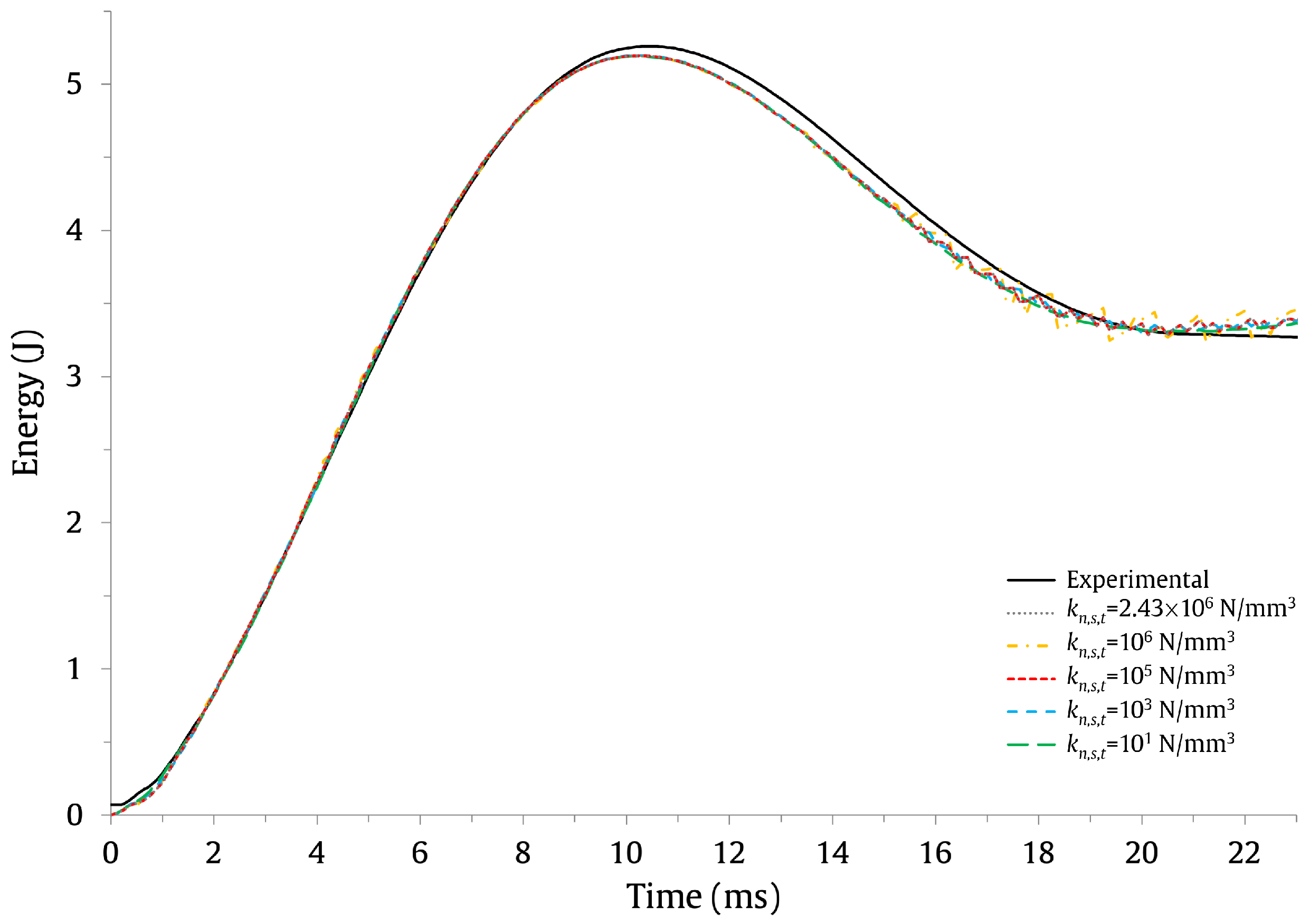
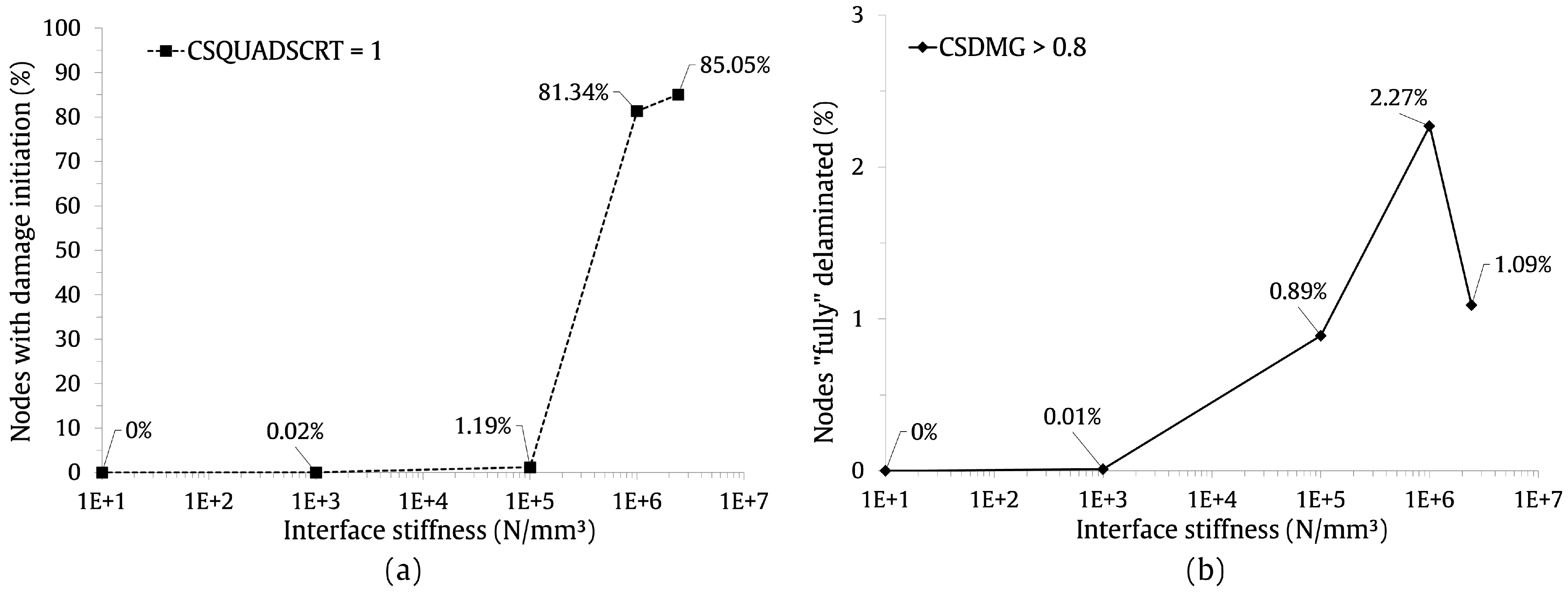
3.1. Effect of the Interface Stiffness

To assess the influence of the interface stiffness on the impact response of the semicylindrical woven composite shells, simulations were carried out using cohesive stiffness values ranging from 10${}^1$ N/mm${}^3$ to $2.43\times {10}^6$ N/mm${}^3$ ($k_n=k_s=k_t$), while maintaining the normal and shear interface strengths constant (${\tau }_n^0=15$ MPa and ${\tau }_s^0={\tau }_t^0=30$ MPa). Notice that the highest value considered for the cohesive stiffness, that is, $2.43\times {10}^6$ N/mm${}^3$, was obtained by employing the equation proposed by Turon et al. [30]:

$$k=\frac{\alpha E_3}{t}$$

(11)

where t is the thickness of each ply, $E_3$ is the through-thickness elastic modulus, and $\alpha$ is a parameter larger than 1, which, in this study, was set with a value of 50, as suggested in [30]. The cohesive stiffness proposed by Camanho et al. [29] (10${}^6$ N/mm${}^3$) was also analysed in this study.

The numerical and experimental [2] force–time, energy–time, and force–displacement curves are shown in Figure 3, Figure 4 and Figure 5, respectively. It is possible to appreciate that the cohesive stiffness has no impact on the force and energy histories for values between 10${}^3$ N/mm${}^3$ and $2.43\times {10}^6$ N/mm${}^3$, and that there is a satisfactory numerical–experimental correlation within this range. The force–time and force–displacement response curves are significantly affected by employing smaller cohesive stiffness values, such as 10${}^1$ N/mm${}^3$, because the stiff connection between the laminate layers is not ensured. It was noted, however, that the energy–time response curve was unaffected because the numerical output results for the impact energy were calculated based solely on the mass and velocity of the impactor along the established step time, which were defined on the FE models in accordance with the experimental evidence. On the other hand, high cohesive stiffness values caused convergence issues. For instance, adopting a cohesive stiffness of 10${}^9$ N/mm${}^3$ resulted in immediate convergence failure. It should be noted that these findings are in good agreement with those presented by Song et al. in [33].

If the cohesive stiffness is maintained between 10${}^3$ N/mm${}^3$ and $2.43\times {10}^6$ N/mm${}^3$, the impact bending stiffness (IBS), which is determined by the slope of the ascending branch of the force–displacement curves represented in Figure 5 [34], is also hardly affected. Once more, for 10${}^1$ N/mm${}^3$, the IBS significantly declines and completely breaks apart from the experimental evidence.

It was observed that, in terms of computing efficiency, an increase in cohesive stiffness is accompanied by a significant rise in the number of increments required to compute the solution. As an example, it was observed that increasing the cohesive stiffness from 10${}^5$ N/mm${}^3$ to 10${}^6$ N/mm${}^3$ raised the computational cost of the solution by 138%.

The cohesive stiffness was observed to have a limited impact on the response curves when maintained within the range of 10${}^3$–$2.43\times$10${}^6$ N/mm${}^3$. However, it was identified as a critical factor affecting the delamination predictions. To understand and quantify this impact, the effect of the cohesive stiffness on the delamination initiation and progression are shown in Figure 6a,b, respectively. The damage initiation in the cohesive surfaces was measured for this reason using the output variable CSQUADSCRT. This variable shows whether or not the quadratic contact stress damage initiation threshold was met (see Equation (8)). It was anticipated that cohesive surface degradation would start when its value approached 1. The stiffness deterioration, following damage initiation, was measured using the output variable CSDMG. The interface can be thought of as entirely delaminated when it reaches the value of 1. The results are provided as the percentage of nodes with CSQUADSCRT = 1 and percentage of nodes with CSDMG > 0.8.

The findings demonstrate that delamination only appears for cohesive stiffness values greater than 10${}^3$ N/mm${}^3$. In fact, the influence of delamination in the FE model simulations is hardly perceptible up to 10${}^5$ N/mm${}^3$. The percentage of nodes that experience damage initiation (CSQUADSCRT output variable), however, climbs sharply from 1.19% to 85.05% if the value calculated by Equation (11) is considered (2.43 × 10${}^6$ N/mm${}^3$).

The observed trend reveals a direct correlation between the cohesive stiffness and the percentage of nodes exhibiting complete delamination, as indicated by the CSDMG output variable. Notably, as the cohesive stiffness value, denoted as $k_{n,s,t}$, is increased to ${10}^6$ N/mm${}^3$, the proportion of totally delaminated nodes rises to 2.27% of the total number of nodes within the composite shell. However, when the cohesive stiffness is further elevated to $2.43\times {10}^6$ N/mm${}^3$, the percentage decreases to 1.09%. These findings underscore the significant impact of interface stiffness on the accurate delamination predictions. Moreover, upon analysing the calculated values of $\alpha$ for each considered cohesive stiffness, as determined by Equation (11) and listed in in

Table 3. Parameter $\alpha$ for the considered cohesive stiffness values (calculated from Equation (11)).

Cohesive Stiffness (${\mathit{k}}_{\mathit{n},\mathit{s},\mathit{t}}$)	Parameter $\mathit{\alpha }$
$2.43\times {10}^6$ N/mm${}^3$	50
10${}^6$ N/mm${}^3$	21
10${}^5$ N/mm${}^3$	2.1
10${}^3$ N/mm${}^3$	$2.1\times {10}^{-2}$
10${}^1$ N/mm${}^3$	$2.1\times {10}^{-4}$

, it becomes evident that only for 2.43 × 10${}^6$ N/mm${}^3$ and 10${}^6$ N/mm${}^3$ does $\alpha$ exhibit significant higher values than 1, as suggested by Turon et al. [30]. This underscores the importance of evaluating the value of the parameter $\alpha$ utilised in the numerical simulations, in order to obtain proper delamination predictions.

The effect of the interface stiffness on the delamination predictions throughout the entire FE model, and the damage observed on the experimentally tested specimens [2] are plotted in Figure 7 and Figure 8, respectively.

In Figure 7, it is possible to observe that the FE models with cohesive stiffness values ranging from 10${}^1$ N/mm${}^3$ to 10${}^3$ N/mm${}^3$ do not present any discernible signs of delamination. However, the presence of delamination becomes increasingly apparent as the cohesive stiffness surpasses 10${}^5$ N/mm${}^3$. Notably, for a cohesive stiffness of 10${}^6$ N/mm${}^3$, the extent of delamination becomes more severe, extending beyond the impact area and propagating along the longitudinal direction of the composite shell. However, as seen observed in Figure 6b, with a higher cohesive stiffness of $2.43\times {10}^6$ N/mm${}^3$, the delaminated area noticeably reduces compared to the previous analysed case. It is important to note that a satisfactory agreement can be observed between the experimental evidence presented in Figure 8 and the simulation results obtained with a cohesive stiffness of 10${}^6$ N/mm${}^3$.

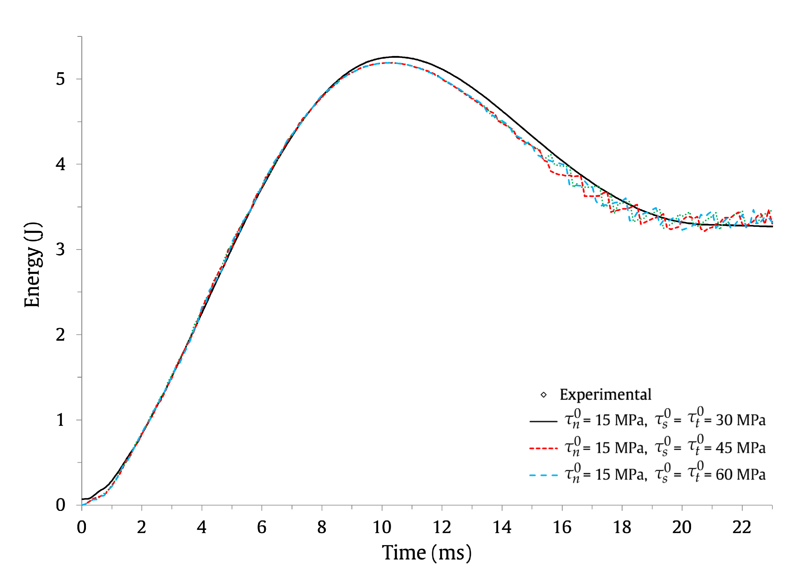
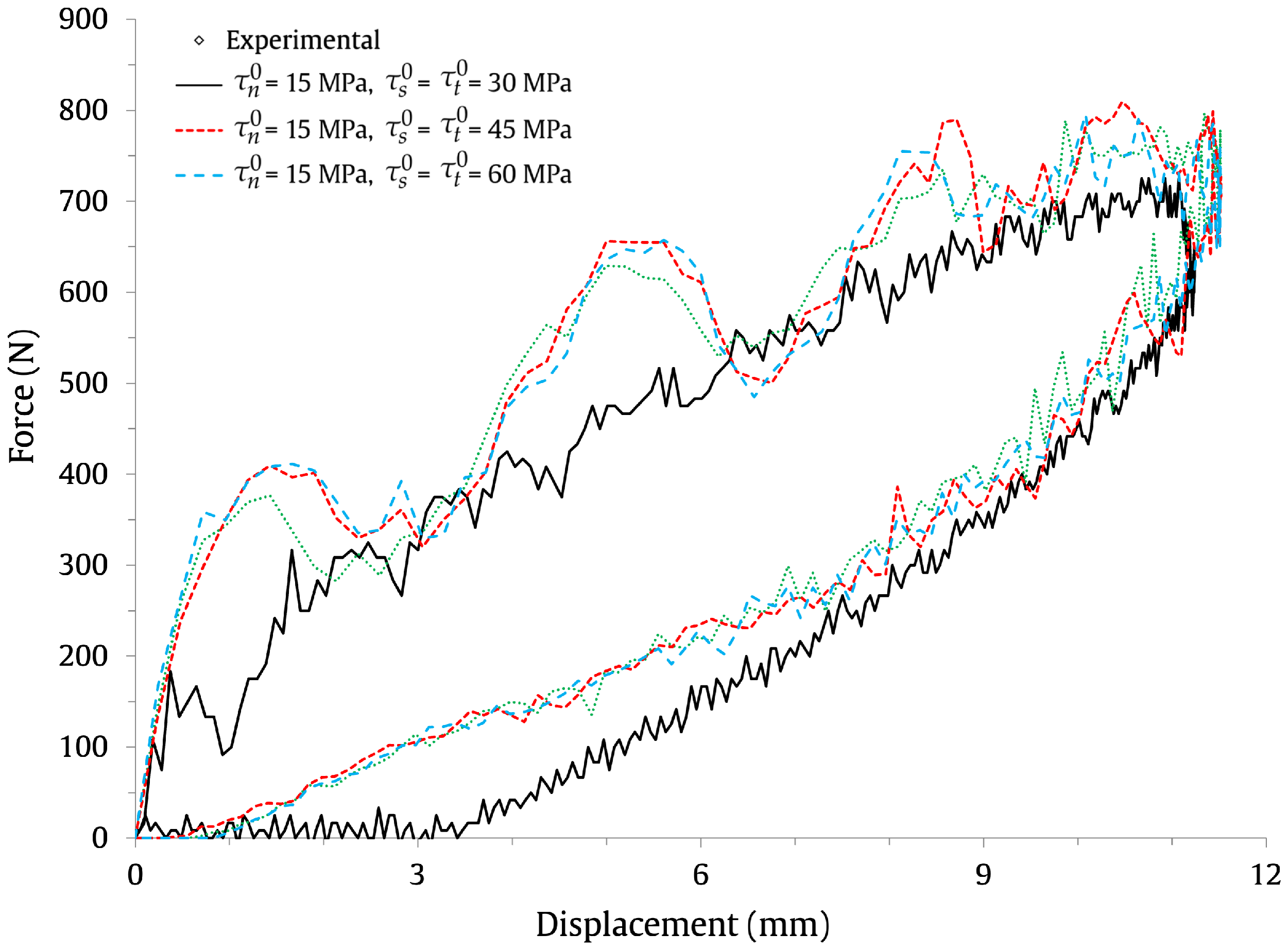
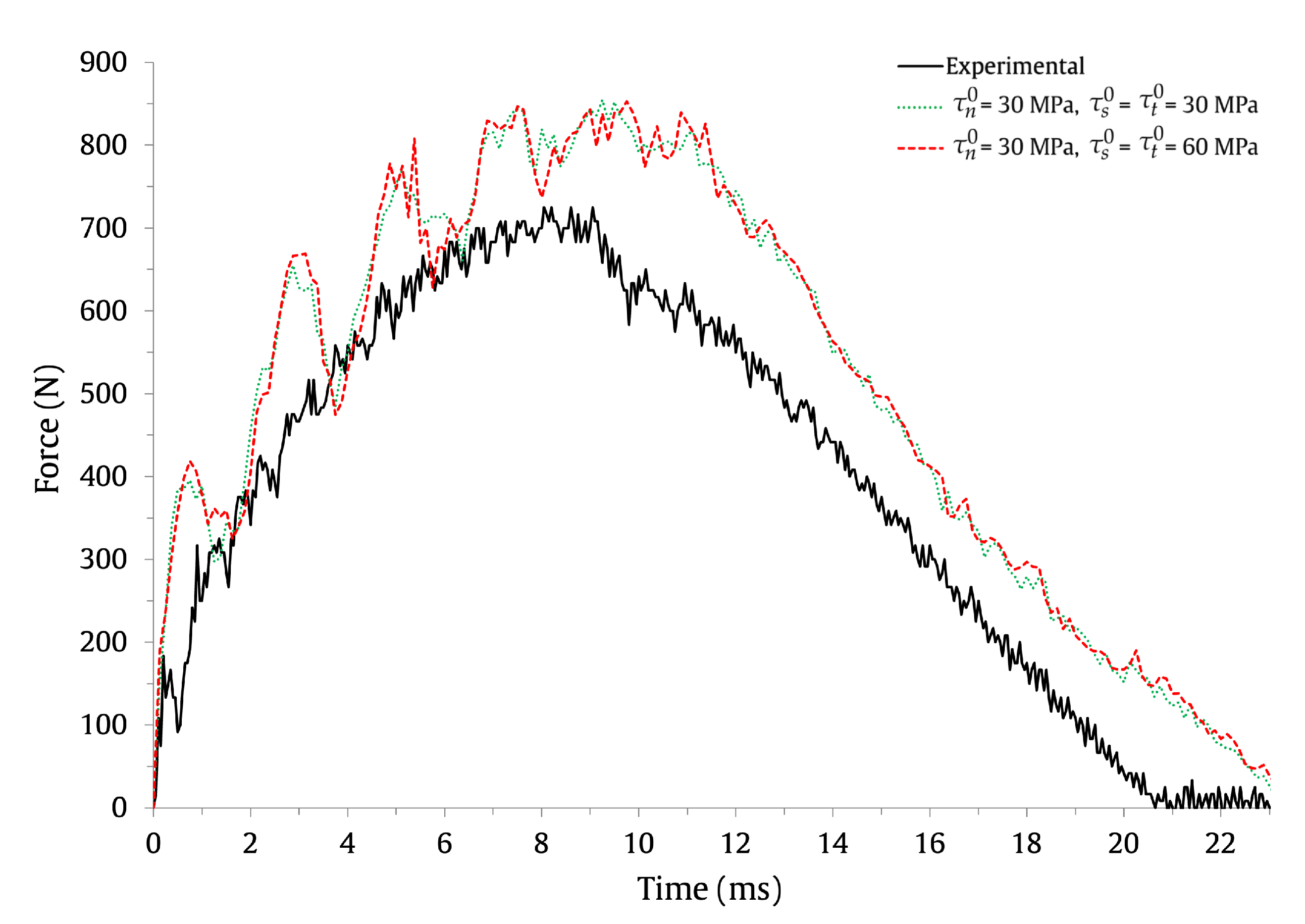
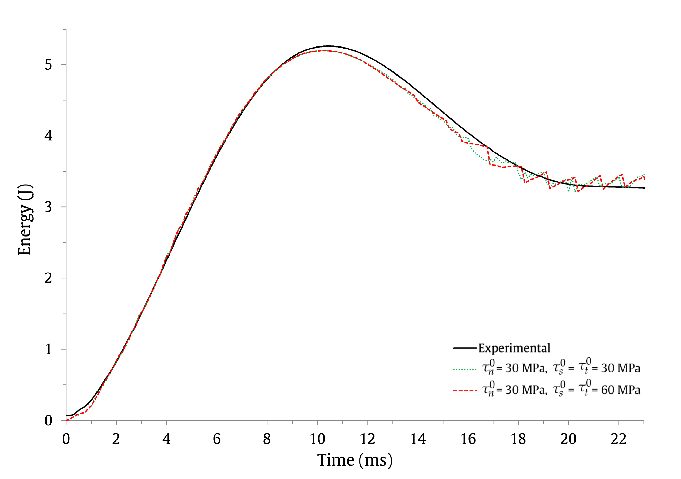
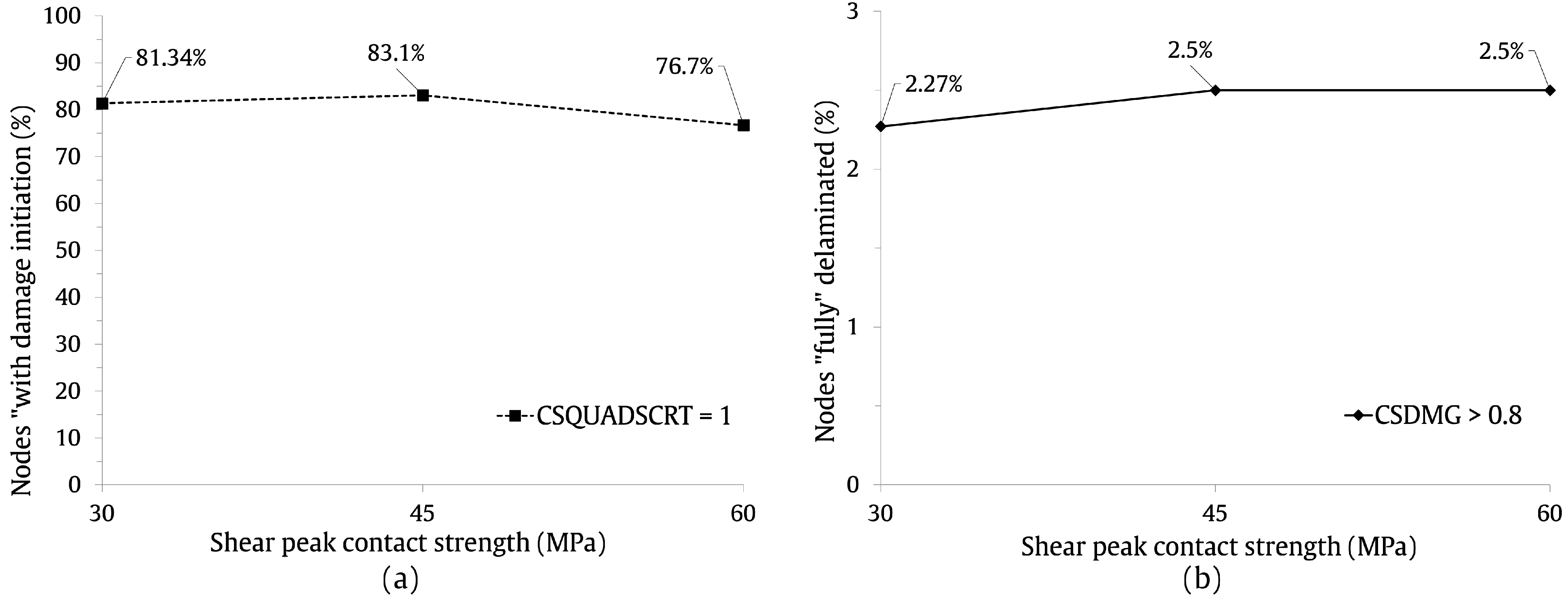
3.2. Effect of the Interface Strength

This section analyses the impact the response curves, delamination, and computing cost of the solutions as a function of the normal peak contact stress ${\tau }_n^0$ and shear peak contact stresses, ${\tau }_s^0={\tau }_t^0$. For that purpose, simulations were carried out in two separate sets, assuming a constant interface stiffness of 10${}^6$ N/mm${}^3$, and in accordance with the values shown in Table 2: (i) with a normal peak contact stress ${\tau }_n^0=15$ MPa and shear peak contact stresses ${\tau }_s^0={\tau }_t^0=30,45,60$ MPa; (ii) with a normal peak contact stress ${\tau }_n^0=30$ MPa and shear peak contact stresses ${\tau }_s^0={\tau }_t^0=30,60$ MPa. The force–time, energy–time, and force–displacement curves are shown in Figure 9, Figure 10 and Figure 11 for the first set, and in Figure 12, Figure 13 and Figure 14 for the second set.

The results demonstrate that adjusting the value of the shear interface strength has a minor impact on the force–time, energy–time, and force–displacement curves for the studied normal interface strengths (${\tau }_n^0=15$ MPa and ${\tau }_n^0=30$ MPa). Additionally, all of the scenarios that were taken into consideration had comparable predictions for the maximum impact force, maximum displacement, and absorbed energy.

On the other hand, it is possible to appreciate how the force–time and force–displacement curves are impacted by changes in the normal contact strength. When the normal contact strength increases from 15 MPa to 30 MPa, the maximum impact force as predicted by the numerical model increases by around 8%. However, as previously indicated, the variation in the normal interface strength has no impact on the maximum displacement and the absorbed energy because the velocity profile was integrated into the FE models according to the experimental results. This interface property, then, has an impact on the agreement between the numerical and experimental findings. A greater numerical–experimental correlation was found for ${\tau }_n^0=15$ MPa than for ${\tau }_n^0=30$ MPa, regardless of the shear interface strength. This discrepancy suggests that the chosen normal strength value of 30 MPa does not accurately capture the true behaviour of the material under investigation. Based on these results, it is evident that caution must be exercised when selecting normal strength values for the numerical model. Therefore, it is crucial to carefully assess and validate the chosen normal strength values to ensure a reliable and meaningful numerical–experimental correlation.

It is also notable that for all the normal and shear interface strength scenarios taken into account, the impact bending stiffness barely changes.

The delamination predictions are also affected by the variation in the normal interface strength. Figure 15 and Figure 16 show, for ${\tau }_n^0=15$ MPa and ${\tau }_n^0=30$ MPa, respectively, the percentage of nodes in the composite shell with the output variables CSQUADSCRT = 1 and CSDMG > 0.8. Moreover, Figure 17 illustrates the extent and location of the delamination predictions in the FE models.

Figure 15a and Figure 16a show that neither the variation in the normal interface strength nor the variation in the shear interface strengths affect the percentage of nodes that achieve the damage initiation threshold. For every case that was looked at, its value is essentially constant and around 80%. It can also be observed in Figure 15b and Figure 16b that, although the amount of fully delaminated nodes decreases as the normal interface strength increases, the effect of changing the shear interface strengths on delamination predictions is less pronounced. In fact, the simulation results show distinct behaviours for the alteration of the shear interface strengths for ${\tau }_n^0=15$ MPa and ${\tau }_n^0=30$ MPa. With an increase in shear interface strengths, the percentage of totally delaminated nodes grows marginally for ${\tau }_n^0=15$ MPa, but it falls for ${\tau }_n^0=30$ MPa. However, the variation is not significant in any situation. The delaminated areas plotted in Figure 17 also support these findings.

The findings demonstrate that the severity and location of delamination are predicted to be identical for all simulations run with ${\tau }_n^0=15$ MPa, remaining, as previously observed, limited to the impact zone and spreading along the length of the shell. This behaviour is still discernible for ${\tau }_n^0=30$ MPa and ${\tau }_s^0={\tau }_t^0=30$ MPa, though much less intensely. However, taking into account greater shear interface strength values led to a noticeably smaller reduction in the observable delaminated areas.

4. Conclusions

In this study, the influence of the interface stiffness and strength on the low-velocity impact response of woven fabric-reinforced composite shells was investigated. For that purpose, FE models that incorporated continuum shell elements and cohesive surfaces to account for the intra- and interlaminar damage, respectively, were generated in ABAQUS/Explicit.

The simulations were performed using interface stiffness values ranging from 10${}^1$ N/mm${}^3$ to $2.43 \times$10${}^6$ N/mm${}^3$ and interface strength values ranging from 15 MPa to 60 MPa. To be able to analyse the results, the force–time, energy–time, and force–displacement curves were presented. Additionally, in order to assess the extent of cohesive degradation and delamination within the FE models, the variation in the percentage of nodes initiating cohesive degradation and the percentage of nodes that become fully delaminated were plotted. It was observed that, for values between 10${}^3$ N/mm${}^3$ and $2.43\times$10${}^6$ N/mm${}^3$, the interface stiffness has a negligible effect on the force and energy histories, and, within this range, there is a satisfactory numerical–experimental correlation. The use of stiffness values outside this range resulted in convergence issues (high values of interface stiffness) or no numerical–experimental correlation (low values of interface stiffness). Although the interface stiffness has a minimal impact on the response curves’ accuracy, it has a significant impact on the delamination predictions. Only for an interface stiffness value of 10${}^5$ N/mm${}^3$ do completely delaminated nodes become clearly visible. Furthermore, it is worth noting that a significant increase in computational cost was observed with the increase in interface stiffness.

The results show that the shear interface strength values (peak contact stresses) have a negligible impact on the force and energy histories. On the other hand, the normal interface strength affects the numerical predictions of the maximum impact force. Increasing its value from 15 MPa to 30 MPa resulted in an 8% increase in the maximum impact force, and thus a deviation from the experimental data. Only the variation in the normal interface strength was found to have an effect on the delamination predictions. It was observed that the percentage of fully delaminated nodes decreases with the increase of the normal interface strength; however, the percentage of nodes that initiate cohesive degradation remains almost unchanged. In addition, it was observed that varying the interface strength had minimal impact on the computational cost of the solutions.

The results obtained from this study provide valuable insights and recommendations for accurately and efficiently simulating delamination phenomena. By successfully validating the FE models used in this research, a strong basis is established for conducting future numerical investigations. It also presents an opportunity to reduce the reliance on costly and time-consuming experimental testing. Furthermore, the utilisation of numerical simulations enables researchers to investigate delamination in a more detailed and comprehensive manner. The FE models can capture intricate delamination mechanisms, predict failure modes, and provide detailed information about stress distribution and energy absorption during the process. This information can be utilised to enhance design guidelines, develop mitigation strategies, and optimise the performance and reliability of laminated shell structures.

References

1. Ferreira, L.; Coelho, C.; Reis, P. Impact Response of Semi-Cylindrical Composite Laminate Shells Under Repeated Low-Velocity Impacts. In Proceedings of the 2022 Advances in Science and Engineering Technology International Conferences (ASET), Dubai, United Arab Emirates, 21–24 February 2022; pp. 1–5. [Google Scholar] [CrossRef]
2. Reis, P.; Sousa, P.; Ferreira, L.; Coelho, C. Multi-impact response of semicylindrical composite laminated shells with different thicknesses. Compos. Struct. 2023, 310, 116771. [Google Scholar] [CrossRef]
3. Amaro, A.M.; Reis, P.N.B.; de Moura, M.F.S.F.; Santos, J.B. Damage detection on laminated composite materials using several NDT techniques. Insight 2012, 54, 14–20. [Google Scholar] [CrossRef]
4. ASTM D7136/D7136M-05; Standard Test Method for Measuring the Damage Resistance of a Fiber Reinforced Polymer Matrix Composite to a Drop Weight Impact Event. American Society for Testing and Materials. ASTM: Philadelphia, PA, USA, 2005.
5. Richardson, M.; Wisheart, M. Review of low-velocity impact properties of composite materials. Compos. Part A Appl. Sci. Manuf. 1996, 27, 1123–1131. [Google Scholar] [CrossRef]
6. Ferreira, L.; Coelho, C. Modelling Progressive Damage in NCF Composites using the Continuum Damage Mechanics Method. In Proceedings of the 2022 Advances in Science and Engineering Technology International Conferences (ASET), Dubai, United Arab Emirates, 21–24 February 2022; pp. 1–4. [Google Scholar] [CrossRef]
7. Ferreira, L.M.; Graciani, E.; París, F. Modelling the waviness of the fibres in non-crimp fabric composites using 3D finite element models with straight tows. Compos. Struct. 2014, 107, 79–87. [Google Scholar] [CrossRef]
8. Ferreira, L.M.; Graciani, E.; París, F. Predicting failure load of a non-crimp fabric composite by means of a 3D finite element model including progressive damage. Compos. Struct. 2019, 225, 111115. [Google Scholar] [CrossRef]
9. Ferreira, L.M.; Graciani, E.; París, F. Three dimensional finite element study of the behaviour and failure mechanism of non-crimp fabric composites under in-plane compression. Compos. Struct. 2016, 149, 106–113. [Google Scholar] [CrossRef]
10. de Moura, M.; Campilho, R.; Amaro, A.; Reis, P. Interlaminar and intralaminar fracture characterization of composites under mode I loading. Compos. Struct. 2010, 92, 144–149. [Google Scholar] [CrossRef]
11. Kim, S.J.; Goo, N.S.; Kim, T.W. The effect of curvature on the dynamic response and impact-induced damage in composite laminates. Compos. Sci. Technol. 1997, 57, 763–773. [Google Scholar] [CrossRef]
12. Choi, I.H. Finite element analysis of low-velocity impact response of convex and concave composite laminated shells. Compos. Struct. 2018, 186, 210–220. [Google Scholar] [CrossRef]
13. Zhao, G.; Cho, C. On Impact Damage of Composite Shells by a Low-Velocity Projectile. J. Compos. Mater. 2004, 38, 1231–1254. [Google Scholar] [CrossRef]
14. Kistler, L.S.; Waas, A.M. Experiment and Analysison the Response of Curved Laminated Composite Panels Subjected to Low Velocity Impact. Int. J. Impact Eng. 1998, 21, 711–736. [Google Scholar] [CrossRef]
15. Kumar, S.; Nageswara Rao, B.; Pradhan, B. Effect of Impactor Parameters and Laminate Characteristics on Impact Response and Damage in Curved Composite Laminates. J. Reinf. Plast. Compos. 2007, 26, 1273–1290. [Google Scholar] [CrossRef]
16. Ferreira, L.M.; Coelho, C.A.C.P.; Reis, P.N.B. Numerical Simulations of the Low-Velocity Impact Response of Semicylindrical Woven Composite Shells. Materials 2023, 16, 3442. [Google Scholar] [CrossRef] [PubMed]
17. ABAQUS Analysis User’s Manual, Version 6.14; Dassault Systèmes Simulia Corp: Providence, RI, USA, 2014.
18. ABAQUS/Explicit. VUMAT for Fabric Reinforced Composites; Dassault Systèmes Simulia Corp: Providence, RI, USA, 2008.
19. Johnson, A.; Pickett, A.; Rozycki, P. Computational methods for predicting impact damage in composite structures. Compos. Sci. Technol. 2001, 61, 2183–2192. [Google Scholar] [CrossRef] [Green Version]
20. Ladeveze, P.; LeDantec, E. Damage modelling of the elementary ply for laminated composites. Compos. Sci. Technol. 1992, 43, 257–267. [Google Scholar] [CrossRef]
21. Liu, X.; Rouf, K.; Peng, B.; Yu, W. Two-step homogenization of textile composites using mechanics of structure genome. Compos. Struct. 2017, 171, 252–262. [Google Scholar] [CrossRef]
22. Sridharan, S.; Pankow, M. Performance evaluation of two progressive damage models for composite laminates under various speed impact loading. Int. J. Impact Eng. 2020, 143, 103615. [Google Scholar] [CrossRef]
23. Bodepati, V.; Mogulanna, K.; Rao, G.S.; Vemuri, M. Numerical Simulation and Experimental Validation of E-Glass/epoxy Composite Material under Ballistic Impact of 9 mm Soft Projectile. Plast. Impact Mech. 2017, 173, 740–746. [Google Scholar] [CrossRef]
24. Esnaola, A.; Elguezabal, B.; Aurrekoetxea, J.; Gallego, I.; Ulacia, I. Optimization of the semi-hexagonal geometry of a composite crush structure by finite element analysis. Compos. Part B Eng. 2016, 93, 56–66. [Google Scholar] [CrossRef]
25. Kostopoulos, V.; Markopoulos, Y.; Giannopoulos, G.; Vlachos, D. Finite element analysis of impact damage response of composite motorcycle safety helmets. Compos. Part B Eng. 2002, 33, 99–107. [Google Scholar] [CrossRef]
26. Hoo Fatt, M.S.; Lin, C. Perforation of clamped, woven E-glass/polyester panels. Compos. Part B Eng. 2004, 35, 359–378. [Google Scholar] [CrossRef]
27. Alonso, L.; Martínez-Hergueta, F.; Garcia-Gonzalez, D.; Navarro, C.; García-Castillo, S.; Teixeira-Dias, F. A finite element approach to model high-velocity impact on thin woven GFRP plates. Int. J. Impact Eng. 2020, 142, 103593. [Google Scholar] [CrossRef]
28. Benzeggagh, M.; Kenane, M. Measurement of mixed-mode delamination fracture toughness of unidirectional glass/epoxy composites with mixed-mode bending apparatus. Compos. Sci. Technol. 1996, 56, 439–449. [Google Scholar] [CrossRef]
29. Camanho, P.P.; Davila, C.G.; de Moura, M.F. Numerical Simulation of Mixed-Mode Progressive Delamination in Composite Materials. J. Compos. Mater. 2003, 37, 1415–1438. [Google Scholar] [CrossRef]
30. Turon, A.; Dávila, C.; Camanho, P.; Costa, J. An engineering solution for mesh size effects in the simulation of delamination using cohesive zone models. Eng. Fract. Mech. 2007, 74, 1665–1682. [Google Scholar] [CrossRef]
31. Schön, J. Coefficient of friction of composite delamination surfaces. Wear 2000, 237, 77–89. [Google Scholar] [CrossRef]
32. Bresciani, L.; Manes, A.; Ruggiero, A.; Iannitti, G.; Giglio, M. Experimental tests and numerical modelling of ballistic impacts against Kevlar 29 plain-woven fabrics with an epoxy matrix: Macro-homogeneous and Meso-heterogeneous approaches. Compos. Part B Eng. 2016, 88, 114–130. [Google Scholar] [CrossRef]
33. Song, K.; Dávila, C.G.; Rose, C.A. Guidelines and parameter selection for the simulation of progressive delamination. In Proceedings of the 2008 Abaqus Users’ Conference, Newport, RI, USA, 19–22 May 2008; Volume 41, pp. 43–44. [Google Scholar]
34. David-West, O.; Nash, D.; Banks, W. An experimental study of damage accumulation in balanced CFRP laminates due to repeated impact. Compos. Struct. 2008, 83, 247–258. [Google Scholar] [CrossRef]
Figure 1. FE modelling approach based on continuum shell elements and cohesive surfaces: (a) Representation of the complete FE model. (b) Schematic representation of the shell in the through-thickness direction. The parameter t refers to the thickness of a layer.
Applsci 13 06948 g001
Figure 2. Bilinear cohesive model for mixed modes (normal and shear modes).
Applsci 13 06948 g002
Figure 3. Effect of the interface stiffness on the force–time results with τ n 0 = 15 MPa and τ s 0 = τ t 0 = 30 MPa.
Applsci 13 06948 g003
Figure 4. Effect of the interface stiffness on the energy–time results with τ n 0 = 15 MPa and τ s 0 = τ t 0 = 30 MPa.
Applsci 13 06948 g004
Figure 5. Effect of the interface stiffness on the force–displacement results with τ n 0 = 15 MPa and τ s 0 = τ t 0 = 30 MPa.
Applsci 13 06948 g005
Figure 6. Effect of the interface stiffness with τ n 0 = 15 MPa and τ s 0 = τ t 0 = 30 MPa: (a) CSQUADSCRT output variable. (b) CSDMG output variable.
Applsci 13 06948 g006
Figure 7. Effect of interface stiffness on the delamination predictions with τ n 0 = 15 MPa and τ s 0 = τ t 0 = 30 MPa, represented throughout the FE model.
Applsci 13 06948 g007
Figure 8. Damage observed on the experimentally tested specimens (visual inspection with intense backlight) [2].
Applsci 13 06948 g008
Figure 9. Effect of the interface strength on the force–time results for τ n 0 = 15 MPa and k n = k s = k t = 10 6 N/mm 3 .
Applsci 13 06948 g009
Figure 10. Effect of the interface strength on the energy–time results for τ n 0 = 15 MPa and k n = k s = k t = 10 6 N/mm 3 .
Applsci 13 06948 g010
Figure 11. Effect of the interface strength on the force–displacement results with τ n 0 = 15 MPa and k n = k s = k t = 10 6 N/mm 3 .
Applsci 13 06948 g011
Figure 12. Effect of the interface strength on the force–time results with τ n 0 = 30 MPa and k n = k s = k t = 10 6 N/mm 3 .
Applsci 13 06948 g012
Figure 13. Effect of the interface strength on the energy–time results with τ n 0 = 30 MPa and k n = k s = k t = 10 6 N/mm 3 .
Applsci 13 06948 g013
Figure 14. Effect of the interface strength on the force–displacement results with τ n 0 = 30 MPa and k n = k s = k t = 10 6 N/mm 3 .
Applsci 13 06948 g014
Figure 15. Effect of the interface stiffness with τ n 0 = 15 MPa and k n = k s = k t = 10 6 N/mm 3 : (a) CSQUADSCRT output variable. (b) CSDMG output variable.
Applsci 13 06948 g015
Figure 16. Effect of the interface stiffness with τ n 0 = 30 MPa and k n = k s = k t = 10 6 N/mm 3 : (a) CSQUADSCRT output variable. (b) CSDMG output variable.
Applsci 13 06948 g016
Figure 17. Effect of interface strength on the delamination predictions with k n = k s = k t = 10 6 N/mm 3 , represented throughout the FE model.
Applsci 13 06948 g017