1. Introduction
Nowadays, smartphones have become necessary devices in our daily lives. With their widespread use, every day applications are using our location. For instance, we can quickly navigate using an online service such as Google Maps. However, indoor navigation is limited, since Global Navigation Satellite System (GNSS) signals are attenuated in indoor environments. Furthermore, a comprehensive database of indoor maps needs to be developed.
The use of indoor location is critical in various industries. Thus, many methods have been developed for indoor localization. For example, there are localization methods using indoor image databases [
1,
2], lighting information of the environment [
3], the magnetic field of the structure [
4], the Received Signal Strength Indication (RSSI) from Wi-Fi access points, and Bluetooth Low Energy (BLE) beacons installed inside a building [
5,
6]. However, these methods require special equipment and fingerprinting maps, which need periodic system maintenance following environmental changes. Maintenance is a heavy burden for managers. Although there is a method that does not require special equipment [
7], it accumulates localization errors estimated by Pedestrian Dead Reckoning (PDR), resulting in inaccurate localization. In summary, existing methods encounter two obstacles: the maintenance of special equipment and the accumulation of localization errors.
In this paper, we aim to solve these two problems. The proposed method is based on work in [
7]. Specifically, the proposed method uses only smartphones to estimate positions in a map image taken from an information board. Thus, the requirement for special equipment is avoided.
In addition, the error accumulation is suppressed by collaborative indoor localization. Specifically, we propose a method to exchange estimated localization using Bluetooth Low Energy (BLE)-enabled smartphones when users encounter each other. As shown in
Figure 1, either of the phones can estimate a more accurate location, and the other can correct its location using the encounter place detected by BLE. There exists methods using encounter communication [
8,
9]. However, these methods do not fully utilize the estimated locations, as explained in
Section 2.2. The proposed method compares the accuracy of the estimated locations using a machine learning model. Then, the localization performance is improved by the comparison result.
The contributions of this paper are described in the following three points:
A reliable encounter communication architecture using BLE-enabled smartphones.
A model trained on synthesized data for comparing the localization of two users.
A collaborative localization method by adjusting the localization parameters according to the comparison results.
The experiments were carried out at eight facilities. The results showed that the proposed localization comparison method achieved 83.0% localization accuracy. Furthermore, the proposed collaborative localization improved the baseline method by 13.0%.
2. Related Work
There are various approaches to realize indoor localization using a variety of modalities, such as Inertial Measurement Units (IMU), image analysis, and wireless communication. We briefly describe them.
2.1. Inertial Measurement Unit-Based Localization
Pedestrian Dead Reckoning (PDR) is a method of localization using IMU sensors such as accelerometers, gyroscopes, and magnetometers in the smartphone [
10,
11]. SmartPDR [
11] obtains the user’s stride length using the relationship between stride and the magnitude of acceleration along the z-axis. The heading direction is determined by integrating the angular velocity obtained from the gyroscope and the value of the magnetometer.
Some methods process IMU sensor data with Deep Neural Networks (DNNs) such as CNNs to obtain the user’s velocity vector [
12,
13,
14,
15,
16,
17]. RoNIN [
14] uses accelerometer and gyroscope values from a smartphone as input. This method uses Visual Simultaneous Localization and Mapping (SLAM) trajectories as the training data to learn the trajectory of the user. Thus, the method uses velocity vectors to predict daily activities, such as walking, putting the device in a pocket, etc.
IMU-based methods suffer from error accumulation since localization is relative to the start position. Thus, the localization quality deteriorates significantly when the user walks a long distance. Therefore, the proposed method suppresses error accumulation by exploiting a new collaborative technique.
2.2. Localization with Indoor Maps
In order to reduce the localization error in IMUs or other approaches, there exist methods to utilize indoor maps [
18,
19]. These methods perform localization by combining indoor maps and map matching algorithms with a particle filter [
7,
20,
21]. Map matching localizes the user’s position on the indoor map. Precisely, the methods predict the user’s walking trajectory on the indoor map by a particle filter using IMU data. The particles hold parameters such as position, orientation, and scale, which are successively updated by the velocity vectors obtained from the IMU. Each particle has a weight, representing confidence in the user’s location. Then, the position on the indoor map is calculated by the weighted average over the positions of the particles. Generally, the weight needs to be small if particles pass through the obstacles in the indoor map, such as a wall in the floor plan. Rormero et al. [
20] calculated the overlap of obstacles with the trajectory. Then, the weight was decided according to the degree of the overlap.
The methods in [
7,
18,
19,
20,
21] use indoor maps and map matching to reduce error accumulation. However, the localization fails if the error accumulation is too large and the indoor map is distorted. The proposed collaborative method solves this problem using the information from the other device.
2.3. Wireless-Based Localization
There is a localization approach using radio waves from Wi-Fi access points or Bluetooth beacons. The trilateration method identifies the position using three or more transmitters whose positions are known [
22]. The position is an intersection of radio waves emitted by three transmitters. Localization by triangulation exploiting the Angle of Arrival (AOA) is also available [
23]. However, the methods using radio waves are inaccurate since radio waves go through multiple paths in indoor environments due to wall reflection.
Several localization methods using Wi-Fi fingerprints have been developed [
5,
6]. These methods compile a database composed of RSSIs, which are related to indoor locations. Generally, the database is called the fingerprint. Localization is performed by matching an observed RSSI with the fingerprint. However, the construction of the fingerprint requires a large amount of human work.
There are methods of communicating with other users to improve the localization accuracy. Kloch et al. [
8] corrected their location by merging the probability distributions for their own and others’ locations when users encountered each other. Qiu et al. updated the weights of a particle filter using the distance between their own device and other devices [
9]. However, these methods only consider current locations. Previous locations are an informative resource to correct the current location. The proposed method analyzes various information in multiple steps to achieve a highly accurate localization.
3. Proposed Method
We propose a novel collaborative mechanism to reduce the cumulative error of localization by communicating between smartphones when two users encounter each other. As shown in
Figure 2, the proposed method comprises three modules: encounter communication, localization comparison at the encounter location, and localization correction.
We acquire walking data, stride length, and heading direction using SmartPDR [
11]. Then, the indoor position is estimated by projecting the walking data to an indoor map obtained from the information board image. Inspired by localization using indoor maps [
7], a particle filter is used to project walking data to the map image. If the encounter of users is detected, we compare the trajectories of estimated locations by a decision tree model trained on synthesized walking data. Finally, the positions are corrected according to the comparison result.
3.1. Baseline Localization Using a Particle Filter
We were inspired to adopt a particle filter by existing methods [
24,
25,
26] with a particle filter for estimating the user’s position in a map image. Additionally, particle filters are used in a wide range of tasks, such as multiple target tracking [
27], magnetic particle tracking [
28], and wireless tracking of magnet position [
29]. The Kalman filter is also a promising algorithm for the localization task [
30,
31].
We manually create the passage region, which consists of 0 or 1 values, from the image of the information board. Given a stride length
l and a heading direction
, one particle follows Equation (
1) to update three parameters: the two-dimensional position
in the map image, the scale of the map
(meter-per-pixel), and the offset of the heading direction
. This converts the coordinates of the smartphone to the map image.
denotes noise from a normal distribution. Likewise, the sine function is used for updating
y. Furthermore,
and
are updated by adding noise obtained from normal distributions. Finally, the position is defined as the average of the positions of all the particles. The number of particles is 2000. Particles will disappear if they are not in the passage region. Resampling is performed to keep the total number of particles constant. We followed the work in [
7] to determine the number of particles. The proposed method removes particles if they are not in the passage regions. Thus, localization will fail if all the particles are removed at once. The experimental results verified that localization was performed successfully. All particles did not disappear at once. Therefore, the number of particles was sufficient.
3.2. Encounter Communication Using Bluetooth Low Energy (BLE)
Indoor localization using Bluetooth Low Energy (BLE) is an essential technology that is used in various indoor applications, such as emergency management [
32], occupancy tracking [
33], smart grids [
34], and smart energy management [
35] in buildings. In this paper, BLE is used to detect the user’s encounters and exchange the user’s localization performance, resulting in a realization of a collaborative localization.
A novel method of encounter communication is devised for two users using BLE. There are two modes in BLE: broadcasting and connection. Generally, the broadcast mode is used for encounter communication. However, we experimentally confirmed that the relationship between the RSSI and distance is more stable in the connection mode. Hence, the connection mode is used to realize encounter communication. In connection mode, the device has two roles: central and peripheral. The central mode scans packets and initiates a connection. The peripheral mode sends request packets and follows the central to exchange data. Communication is established only between the central and peripheral modes. In addition, devices cannot communicate with other devices if they have the same role. Therefore, we develop an application that operates both central and peripheral modes. The application chooses a suitable role dynamically. The flow of the proposed encounter communication is shown in
Figure 3. The application has a unique number for each device. Here, the device operates the central mode at the beginning of the communication if it has a larger number than the other. Thus, communication can be prevented from being unstable due to the establishment of multiple communications between devices.
An encounter is detected using the relationship between the RSSI and distance.
Figure 4 shows an example of a relationship measured in the connection mode. A Google Pixel 4a was used. Specifically, we detect an encounter when an average of three consecutive RSSI values are larger than a threshold. The threshold is set to −58 (dBm) in this study. For example, the encounter interval is from one to four meters in
Figure 4. Communication is not established for 10 s after the previous communication to prevent multiple communications with the same collaborator immediately after the data exchange. In other words, the communication will not be re-connected for 10 s. Thus, an encounter will not be detected if the two devices re-encounter right after they first meet. Multiple and immediate re-encounters are not assumed in this work.
3.3. Localization Comparison
After an encounter is detected, the localization accuracies of two devices are compared using a machine learning model. Generally, models require large amounts of training data. However, actual walking data are difficult to obtain comprehensively. Therefore, we synthesize walking data and perform the baseline method to generate training data.
Data generation is described in
Section 3.3.1. Furthermore, feature extraction and the machine learning model for localization comparison are described in
Section 3.3.2 and
Section 3.3.4, respectively.
3.3.1. Generation of Walking Data
We generate walking data (stride length and heading direction per step) by connecting intersections in the map.
Firstly, as shown in
Figure 5, a walking path is generated using an information board. We manually extract the passage region from the board image, resulting in a binary image (one if the pixels are in a passage region, zero otherwise). Intersections in the passage are defined by hand, and paths are created by connecting the intersections. We can dynamically create a walking path by finding a route connecting two randomly selected intersections.
Secondly, we generate walking data using a created walking path as shown in
Figure 5c. Positions on the walking path are determined with the interval of 0.6 m, which is an approximate human stride length. Seven scales of the map
are used to project the interval to the map image. In addition, random noise is generated in the positions since map distortion and PDR errors cause a discrepancy between the actual and generated walking paths.
Finally, sets of stride lengths and heading directions are obtained using the determined positions. For example, the stride length at time i is defined as , where represents the position in the map image. Likewise, the heading direction is .
3.3.2. Feature Extraction from Localization Process
We extract 15 features expressed in
Table 1 from the localization process of the baseline method. Broadly, the features can be grouped into four categories. The features are developed by focusing on a position where a user makes a turn. We detect a turning position
from the walking data if Equation (
2) is satisfied [
36]. The turning position is useful for evaluating the localization quality. For instance, the localization quality is poor if there is a large gap between the turning position and the nearest intersection. Furthermore, disappearing particles are essential features. The presence of disappearing particles means there is a very low possibility that the device will be located at those certain positions, which indicates that the device is very likely passing through an obstacle. Moreover, large variations in the particle parameters indicate that a variety of particles are required to correct the localization. Since the results obtained by PDR are relative positions, errors accumulate as the number of steps increases.
3.3.3. Evaluation Metric for Localization
Estimated positions are evaluated using a metric
M defined in Equation (
3). Specifically, we use the Dynamic Time Warping distance
D [
37] to measure the distance between the estimated positions
and the ground truth (GT) position
.
is created by selecting points on the walking path with a fixed interval, which divides the path equally. We used sampling points of the GT path to match estimated positions to appropriate points on the GT. For example, as shown in
Figure 6, the estimated positions in the red dashed circle should be matched to the two points, respectively. If the GT path is used, the estimated two points will be matched to close points on the GT path, resulting in incorrect matches.
is the number of matching elements of the series
and
. A smaller metric is better.
3.3.4. Comparison Method Using Machine Learning
Localization qualities are compared by a decision tree model as shown in
Figure 7. Specifically, we use a gradient boosting framework, LightGBM [
38]. The effectiveness of the gradient-boosting machine (GBM) algorithm has been verified in a wide range of tasks, such as binary classification [
39], multi-class classification [
40,
41], and fault detection [
42]. Additionally, we considered the efficiency of the algorithm since a mobile device is used to run the model.
We compared two localization processes, A and B. The features are extracted from each process and concatenated to make input features for the model. The label value zero is assigned to the input features if the metric of the process A is smaller than B. Therefore, the model is trained by solving a binary classification task. The output of the model is a value ranging from 0 to 1.
The model is trained on only the synthesized walking data. Two localization processes are performed on the same map image and . We allow no encounters between the processes. Thus, the model compares independent localization processes.
3.4. Collaborative Localization Correction
Particles are corrected using the encountered user’s position and the comparison model’s output. The two users are close to each other when an encounter is detected. Therefore, we can correct the localization of both encountered users by replacing the position of some particles
with the position of the collaborator
. Here, we assume that both devices use the same map for localization. Equation (
4) is used to determine the number of particles to be corrected according to the comparison output
o, which represents the collaborator’s localization quality against their own localization.
is the total number of particles in their own device. For example, when
, 20% of the position of particles
are replaced with the collaborator’s position
.
m is used to consider the deviation of the distance between users during the encounter (and positioning errors). Accordingly, the position of the particle is corrected by
.
The offset
of particles is corrected, since the heading direction can deviate when a localization has significant errors. This offset is determined according to the initial heading direction on the map. Hence, we correct the offset using the offsets of previous particles. Specifically, the offset is updated by Equation (
5). We update 50 % of particles at time
i. The function med represents the median function.
is the average offset in particles at time
i. The average offset
is used to suppress a drastic update.
denotes the standard deviation.
4. Experiments
Three experiments were carried out to evaluate the proposed collaborative localization method, the encounter communication, and the localization comparison.
4.1. Datasets
We developed training and test datasets containing information map images and walking data (stride lengths and heading directions). The map images of twelve and eight facilities were obtained for training and test datasets, respectively.
The training dataset contained the synthesized walking data described in
Section 3.3.1. We generated 50 walking data for each map image and scale
. Then, baseline localization was applied to the walking data ten times to extract the features of localization. Thus, there were 3500 sets of localization results for a map. Two results were selected randomly from the same map at the same scale to generate input features for the comparison model. Consequently, the training dataset contained 42,875 input features for each map. The comparison model was trained using the training dataset.
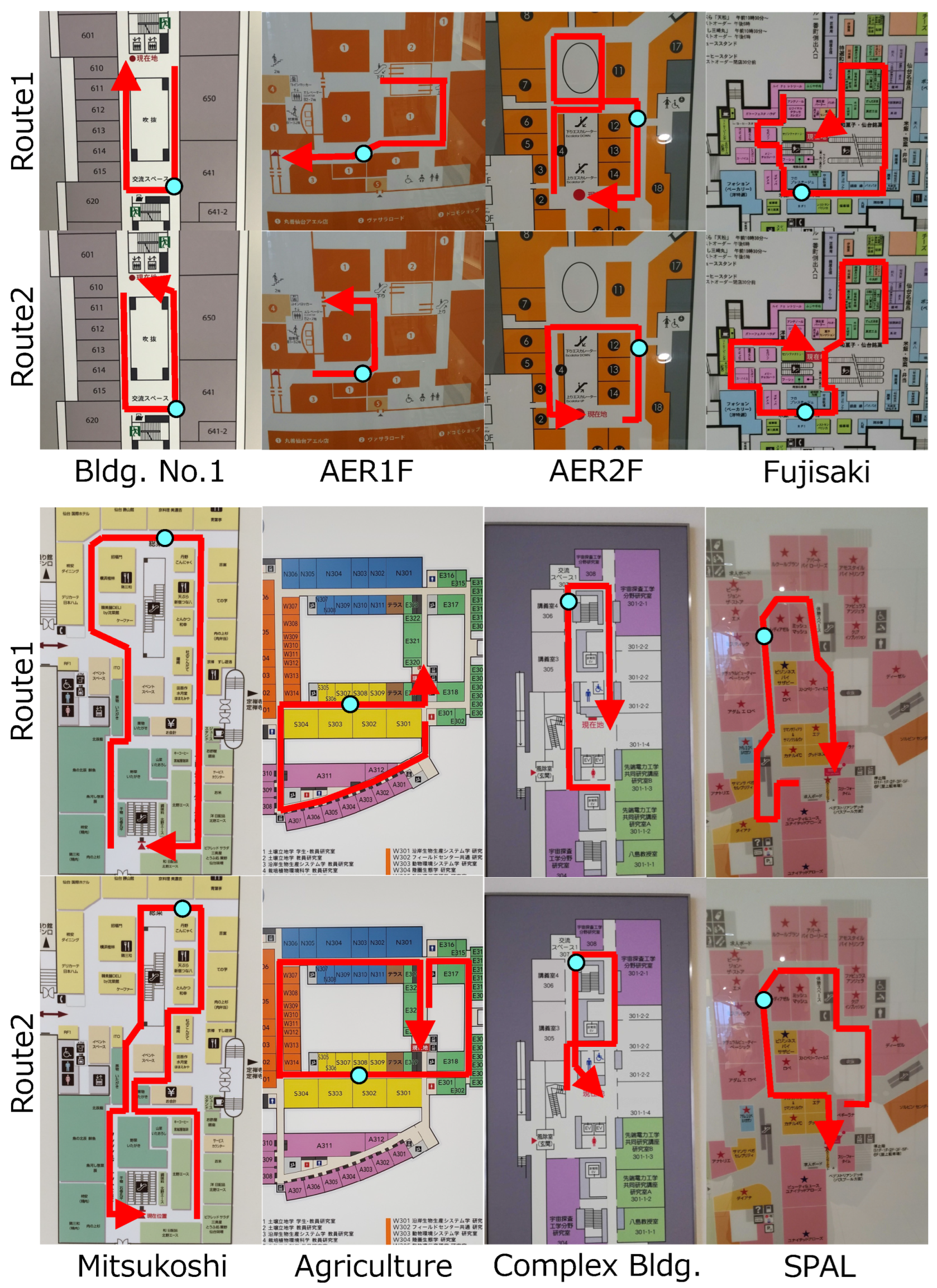
The test dataset was actual walking data obtained by a smartphone, a Google Pixel 4a, at eight facilities. As shown in
Figure 8, there were two walking data properties in a map. The walking data included the time and position of the encounter, which was successfully detected by the proposed method. The walking paths in the map images were determined manually.
4.2. Evaluation on Localization
The proposed method was evaluated in 100 trials using each walking dataset. The evaluation metric for the localization is described in
Section 3.3.3. There are two comparison methods for indoor localization using map images. The first comparison method is the baseline method using PDR and particle filter described in
Section 3.1. The second comparison method, Qiu’s method [
9], improves the baseline method by modifying the weights of particles using encounter communication. When the standard deviation of the collaborator’s particles,
, is within 10 m, the weight of the particle
with index
i is updated by Equation (
6).
is the position of the particle and
represents the estimated location of the collaborator at the encounter. The hyperparameters
and
represent the average and standard deviation of distances between two devices measured by BLE. Values of
and
were determined experimentally.
Table 2 shows the localization results. The proposed method improved the baseline of the average metric by about 18 pixels. On the other hand, the improvement by Qiu’s method was about 2 pixels, which was much smaller than the proposed method. Qiu’s method did not sufficiently utilize the collaborator’s position when modifying the localization. The proposed method exhibited some slight degradations in accuracy, such as route 2 in Fujisaki and Mitsukoshi. Since the collaborator’s position was far from the encounter point, the particles were updated to the wrong positions.
Figure 9 shows an example of the correction for route 1 in Agriculture. The cyan dots are the start positions. The red and blue dots are the estimated position and the turning point, respectively. The red and blue cross marks are the detected encounter positions of the user and its counterpart, respectively. The proposed method correctly estimated the position after collaborative localization correction at the detected encounter. In contrast, the baseline method accumulated errors. Qiu’s method slightly modified the localization using the collaborator’s position. However, the effect of the modification was insufficient.
4.3. Ablation Study on the Collaborative Localization Correction
We evaluated the two modules in the collaborative localization correction, updating the number of particles and the offset using Equations (
4) and (
5), respectively. Specifically,
was fixed to determine the number of particles. Furthermore, the offset was updated by adding a normal distribution:
.
Table 3 shows the improvement rates from the baseline method. Specifically, the improvement rate was calculated by (Baseline − Ours)/Baseline. The full proposed method achieved the highest improvement rate of 13.0%. The method using
achieved the highest improvement rate in route 2 of AER2F and Agriculture. However, there was significant deterioration, for example, for route 2 of Mitsukoshi. The method with
obtained slightly higher improvement rates than the full proposed method on some routes. On the other hand, there was a significant decrease at route 1 in Mitsukoshi.
Figure 10 shows examples of the results. The heading directions significantly deviated in both methods before the encounter. The method with
accumulated error after the encounter, whereas the full proposed method successfully estimated the direction.
4.4. Evaluation of Localization Comparison
The localization comparison model was trained on the training dataset using a cross-entropy loss function. The validation dataset was created by extracting one-quarter of the training dataset and the best model was determined by evaluating the validation dataset. Then, we evaluated the model using the walking data from the start to the encounter in the test dataset. We averaged the results obtained by cross-validation.
Table 4 shows that an accuracy of 0.83 was obtained on the test dataset. Accuracy was low in Building No. 1 and AER2F, where their localizations were highly accurate.
Figure 11 shows examples of comparison pairs of localizations in AER2F. The comparison was correct when the metrics were considerably different. In addition, the number of disappearing particles significantly affected the comparison determination. Many particles disappeared in
Figure 11a. The failed example had two close localizations in the metric. The incorrect result was produced by the features related to turns and intersections.
Figure 11d had a smaller average distance from each turn to the nearest intersection than
Figure 11c.
Figure 12 shows the importance of the features of the comparison model. The importance represents the contribution of each feature to decreasing the loss function. The importance was calculated using the validation dataset. The input features to the model consisted of two localizations. Then, we averaged the corresponding features to obtain the importance of the 15 features.
Generally, the importance I at a node of a decision tree can be calculated by , where L and r represent the loss value at the node and the ratio of the sample size at the node to the total sample size, respectively. Likewise, and are of the left leaf of the node. In this work, binary cross-entropy was used to calculate the loss value. Thus, the importance of a feature f is the total importance at all nodes using f. If the importance is larger, the feature significantly reduces the loss value.
The results showed that the average distance from each turn to the nearest intersection was the most important feature. The proposed method detects the user’s turn positions, and then the distance is measured. Intuitively, the localization performance is high if the predicted turn position is close to the GT intersection. Therefore, the feature is a critical metric for localization performance.
Figure 13 shows the average outputs of the comparison model for correct and incorrect cases. Values were unavailable if there were only correct cases. For simplicity, the output was subtracted from 1 if it exceeded 0.5. Thus, a smaller value indicates a higher confident estimation. In contrast, a value close to 0.5 means an ambiguous estimation. The results showed that the model was more confident for correct than incorrect instances. The outputs in Building No.1 were less confident, since both correct and incorrect were close to 0.5. In fact, the comparison accuracy was the lowest, 0.66, among the facilities. Thus, the model did not make a significant mistake in its estimation on this map.
4.5. Evaluation of Encounter Communication
The encounter communication was evaluated on two facilities in the test dataset. As shown in
Figure 14, two users moved step by step. Then, the distance was measured between the users when an encounter was detected. Ten trials were conducted. The amount of data exchanged at the encounter communication was 500 Bytes.
Table 5 shows the results of the encounter communication. Although the encounter communication failed once, the proposed method successfully detected encounters at an average distance of 1.9 m. The detected distance in Building No.1 was smaller than that for the Complex building. The surrounding walls in the route in Building No.1 are partly made of glass. Thus, the radio waves went through the glass and communication was detected at a close position due to fewer reflected waves.
5. Conclusions
In this paper, we proposed a novel collaborative localization using BLE-based encounter communication. In this encounter communication, an architecture that achieved communication of 500 Bytes was realized. Our method allows multiple communications to be established. We also developed a method to compare the localization of two devices. Virtual walking data were generated and we trained a decision tree model. In addition, we proposed a novel method for correcting the position and direction by using the output value of the comparison. The experimental results showed that the comparison model achieved an 83.0% accuracy for 16 routes at eight facilities. In addition, the proposed method improved the baseline method by 13.0% by appropriately using the collaborator’s location.
The limitation of the proposed method is the manual analysis of map images taken from information boards. In this study, passage regions are manually extracted from the map images. Thus, an automatic method of passage extraction is necessary. A potential approach for automatic extraction is using semantic segmentation models, such as fully convolutional networks [
43] and DeepLabv3+ [
44].


