Abstract
We report composition, grain size, and rheological data related to the mud emitted as a consequence of the maximum moment magnitude (Mw max = 6.5) on 30 October 2016, commonly referred to as the Norcia earthquake (central Italy), and on the activity of pre-existent mud volcanoes affected by the central Italy seismic sequence started on 24 August 2016. The emission sites were located at Monteleone di Fermo and Santa Vittoria in Matenano, two municipalities near the town of Fermo (Marche Region, Italy). We sampled, measured, and analyzed the products of mud emissions 3 days after the mainshock to characterize the mud by geochemical, mineralogical, and rheological analyses. The muds’ geochemical composition and low electrical conductivity suggest a continental origin, likely belonging to the Colombacci Formation. The collected muds are silt–sand–water-rich suspensions characterized by a Bigham rheology with viscosity values between 6.3∙107 and 6.9∙105 Pa∙s. The calculated minimum fluidization velocity of the mud suspensions is between 0.05 m/s (grain size of 2 μm) and 0.74 m/s (grain size of 8 μm). Water-rich mud suspensions flowing on a slope move faster as the water content increases up to 30 wt.%. At higher values, the velocity remains almost constant due to the disaggregation of bonds among the solid particles in the mixtures.
1. Introduction
On 24 August 2016, an earthquake (Mw = 6.2) hit central Italy; its epicenter was close to the village of Accumoli, affecting a very large area, involving four Italian regions: Lazio, Abruzzo, Marche, and Umbria. The earthquake was the first of a strong seismic sequence (Mw max = 6.5), the Amatrice–Norcia–Visso sequence [1,2,3,4,5,6,7]. The area affected by this seismic sequence is between 2 previous seismic events, the 1997 Umbria–Marche Mw 6.0 earthquake in the northwest and the 2009 L’Aquila Mw 6.3 earthquake in the southeast. Indeed, Italy is frequently subject to strong seismic events, sadly noted for the great damage they cause, above all in the zones of the center and south affected by the tectonics of the Apennines. The Amatrice–Norcia–Visso seismic sequence was intense and prolonged, continuing also in 2017. In particular, the 30 October 2016 Mw 6.5 Norcia mainshock was the strongest Italian seismic event since the 1980 Ms 6.9 Irpinia earthquake ([6] and references therein). This earthquake occurred less than 5 km NE of Norcia town as a result of upper crustal normal faulting on a nearly 30 km long, NW-SE-oriented, and SW-dipping fault system (Mt. Vettore–Mt. Bove) [6].
The seismic sequence is the result of the activity of normal faults located along the Apennine ridge. The activated zone is 70 km long and 10 km thick and trends NNW-SSE parallel to the axis of the central–northern Apennines [8]. Each mainshock was followed by sustained aftershock activity; in 3 years, more than 100,000 events were detected by the Italian National Seismic Network (Rete Sismica Nazionale, RSN; http://terremoti.ingv.it/instruments accessed on 2 June 2023), managed by the Istituto Nazionale di Geofisica e Vulcanologia [9]. All these earthquakes have increased attention to seismic risk, engineering applications, and seismic risk mitigation efforts in the affected regions [10]. Unfortunately, each of these events has caused extensive damage to cities and villages as well as large infrastructure systems, especially to historic towns, old urban quarters, villages, and hamlets as well as historic landscapes. In total, there were 299 fatalities, generally due to the collapse of old unrenovated masonry houses. Many localities damaged by the first earthquake on 24 August 2016 were repeatedly shaken and severely damaged by the events that followed, increasing the damage. The October events caused incremental damage to the historic areas, including the total collapse of some structures in several municipalities, and significant damage in many towns in the Apennine foothills. Luckily, the October events resulted in no casualties, as the area had largely been evacuated.
In general, strong earthquakes that can cause widespread territorial and socioeconomic destruction are life-threatening, unexpected, unpredictable, and uncontrollable events with serious psychological consequences [11]. The estimation of the macroeconomic effects of an earthquake critically depends on the identification of the affected area’s boundaries, socioeconomic local heterogeneity, and proper counterfactual analysis [12].
The estimated cost to rebuild the municipalities affected by the seismic sequence that began on 24 August and devastated Lazio, Marche, Umbria, and Abruzzo is more than EUR 26.5 billion. This cost was indicated in a report by the extraordinary commissioner for reconstruction of 2022 and will finance the 56,638 interventions to be carried out in the affected area (https://www.wired.it/gallery/terremoto-2016-italia-amatrice-costo-ricostruzione-dati-commissario/ accessed on 2 June 2023). There are 340,000 damaged buildings scattered over a vast area of 8000 km2, 140 municipalities, more than 70 in the mountains over 900 m asl, and 600,000 people involved.
All the earthquakes, as well as directly damaging the building, cultural, and infrastructural heritage, also have effects on the environment.
Moreover, secondary coseismic effects were induced by the earthquake acceleration after the Norcia earthquake, the strongest seismic event of the entire sequence (Mw = 6.5, occurred on 30 October 2016), including the effusion of mud [7,13] from mud volcanoes and abandoned wells. A wide distribution of mud volcanoes and fluid seeps was observed along the eastern thrust fronts of the Italian peninsula [14]. Different processes can lead to the formation of mud volcanoes, which are usually large structures formed by the eruption of mud breccias pushed to the surface by buoyancy and overpressure, e.g., Mazzini and Etiope [15]. Since the erupting materials are fluid-rich, several types of fluid seepage features are associated with mud volcanoes. The erupted materials essentially consist of solids, water, and gas, the latter being predominantly methane and CO2 (e.g., Kopf [16]). These originated from several phenomena, grouped in with the emission of a mixed mud–water fluid at the surface. Following Kopf [16] and Planke et al. [17], these can be categorized according to morphological features. Mud pools or salsas are collapsed features, and conical edifices are mud extrusions classified on the basis of their height. From a genetic point of view, an anomalous geothermal gradient is not reported at the emission points, and mud volcanism is likely related to the ascent of cold fluids driven by gas-induced overpressures, as is the case of the well-known mud volcanoes along the Pede–Apennine margin of the Northern Apennine, Emilia–Romagna region [2]. Although Emilia–Romagna mud volcanoes have been widely studied, e.g., Bonini [18], Capozzi and Picotti [19,20], Lupi et al. [21], Oppo et al. [22], and Sciarra et al. [23], few documents about the geological and historical activities of mud volcanoes in central Italy are available, such as the emission of saline water and mixtures of mud and hydrocarbons that occur at fractures and small mud volcanoes [24,25,26] along the Marche and the Abruzzo Apennine foothills. As reported above, these phenomena associated with earthquakes are defined as “mud volcanoes”, and we refer to the observations of [27] to describe them. Following these authors, the essential features diagnostic of a mud volcano including the required geological framework of mud volcanism are the occurrence of fossil saline water, evidence of diapirs–diatremes, breccia in the mud discharged, a large amount of mud released, and the major gases have to be related to a catagenetic hydrocarbon production system. Mud volcanism requires thick layers of unconsolidated sediments or brecciated sedimentary rocks with high pore pressures. Mud volcanoes are therefore more common in areas with high sedimentation rates such as sedimentary basins and accretionary prisms. There are hundreds of onshore mud volcanoes [28,29] and a little-known number of offshore mud volcanoes. Faults and fault intersections often help create pathways for fluid upwelling [30]. They are often connected to pressurized hydrocarbon reservoirs, and thus are sometimes the subject of hydrocarbon exploration.
Above, we have outlined that earthquakes may cause gas bubbles’ growth or nucleation, which may encourage the rising of mudflow from deep. The gases detected venting from mud volcanoes are composed predominantly of methane, although some mud volcanoes emit carbon dioxide or nitrogen-enriched gases. Some gases contain dry biogenic methane, others heavier, thermogenic methane (the biochemical gases occur both under surface conditions and at depths up to 1200–2000 m). Usually, the roots of mud volcanoes lay below these depths, and it can be expected that these gases or organic matter will be reworked thermogenically, producing the so-called “thermogenic” gas. The gases of thermogenic origin contain methane accompanied by small amounts of methane homologs and oil leakage. The gases come mainly from source rocks and muddy sediments (clays, shales, mudstones, siltstones, and marls), but shallower layers through which the mud breccia passes may also contribute to the gas. Organic matter makes up a substantial part of freshly deposited mud. Post-depositional transformation leads to active biogenic and thermogenic gas generation, “which is an important added factor which tends to accentuate, or even create, their overpressured, under-compacted state, both by building up additional internal pressure and also by impeding fluid expulsion because of the development of a second phase in the pore fluid” [31]. The high pore fluid pressure is a characteristic feature of all mud volcano areas [31,32] and may be more than twice the hydrostatic pressure and may even be greater than the weight of the overburden.
Therefore, mud volcanoes may be strictly connected to earthquake and fault activity [33]. Indeed, the location and activity of mud volcanoes are sometimes used as indicators of the presence of active fault systems [34]. Earthquakes can influence the rise of mudflow and therefore the eruptions of mud volcanoes by increasing fluid pressure, causing the growth or nucleation of gas bubbles or developing a hydraulic connection between the source or loss of strength, usually located at ~1–3 km depth ([35] and references therein), but greater depths are possible [33], and at the surface [35]. In addition, a close correlation exists between the magnitude of an earthquake and the distance at which a mud volcano eruption can occur ([35] and references therein).
However, in the experimental studies of Manga et al. [35], in which submitted mud suspensions were subjected to cyclic shear under seismic frequencies and amplitudes, the loss of strength occurred at strain amplitudes greater than 10−3, a value much larger than the peak dynamic strain associated with earthquakes that may have triggered mud eruptions. Hanotinm et al. [36] show that applying any finite amplitude vibration suppresses the yield stress of gravitational suspensions that, under vibration, behave as viscous fluids. Their viscosity varies with particle size, suspending fluid viscosity, and vibration amplitude and frequency. However, the real cause/trigger of mud emissions is not well understood. Here, we focus on the case studies of Santa Vittoria in Matenano and Monteleone di Fermo (central Italy) where 17 mud effusions, among the 80 already recognized, erupted shortly after the major earthquakes of the 2016–2017 Amatrice–Norcia–Visso seismic sequence (Figure 1).
Indeed, mud volcanoes are widespread along the Adriatic coast [14]. In the area between the Abruzzo and Marche regions, two main active mud volcano fields are known in Pineto (Pescara province), some smaller ones scattered in the Chieti province, and others in the area near Monteleone di Fermo (Marche region). These small volcanoes produce mudflows and form mud cones a few meters high terminated by a crater. In particular, the village of Monteleone di Fermo is known as the Town of Mud Volcanoes as they are a well-known phenomenon that has been occurring regularly for a long time. There are six emission points located along the Ete Vivo River. Mud volcanoes are induced by the emission of pressurized gas coming from underground deposits of organic material and hydrocarbons [37]. In the Marche region, soon after the Mw 6.5 earthquake, new emission points were detected in Monteleone di Fermo and Santa Vittoria in Matenano, which seem to be further examples of earthquake-triggered/reactivated emission points. In addition, the nearby location of Santa Vittoria in Matenano presented both the reactivation of emission points formed 15 years ago and since then dormant as well as newly formed emission points. Two emission points formed in Contrada San Salvatore, the flow of which covered a wide area and produced large deformations of the neighboring soil. INGV–Emergeo Working Group reconnaissance immediately following the event pointed out that the level of carbon dioxide emissions from the soil was within normal ranges. Low temperatures were measured, a characteristic feature of the phenomenon [37].
This study was aimed to yield new data about one secondary coseismic effect that occurred during the Amatrice–Norcia–Visso sequence: the emission of mud. This goal was reached through (i) analysis of the chemical–physical properties linked to the origin of mud; (ii) determinations of the total water content, grain size distribution, and consequentially the rheological parameters of the emitted mud linked to its motion; and finally (iii) discussions of the physical conditions required to trigger the mud effusions.


Figure 1.
Figure 1a,b is a copy of Figure 1 of Maestrelli et al. [38]. The figure shows (a) the epicenters of earthquakes and (b) the geology of the area and emission centers of mudflows. We added in (c) an image of emission point SV1-A (4766258 N; 375965 E) near the town of Santa Vittoria in Matenano and in (d) an image of emission point ML3-A (43.074429 N; 13.52854 E) near the town of Monteleone di Fermo.


2. Geological Setting and Sampling
The sampling area was located in the Marche Apennine foothills, where turbidite siliciclastic sediments that fill the Messinian foredeep basin are overlapped by Mio–Pliocene marine sediments and Pleistocene continental deposits over it [38,39,40]. The studied area experienced compressional tectonics with NE migration of the Apennine thrust-and-fold belt during the end of the Miocene to the Early Pleistocene. The Messinian turbiditic deposits are mostly composed of pelitic and arenaceous lithofacies containing gypsum intercalations of the Laga Formation. The latter is overlapped by the Colombacci Formation, which is mainly sandy to silty shales intercalated with calcareous levels. The above formations are sharply overlapped by the Pliocene sequence, a marine sequence of alternated mudstone–sandstone lithofacies, i.e., the Argille Azzurre Formation. Quaternary continental deposits lie on top of the marine sequence and outcrop in the Monteleone di Fermo area as a gently deformed NE-dipping monocline [38].
Outcrops of the Argille Azzurre Formation emerge around the Monteleone di Fermo area; however, the formation continues down to considerable depths in the subsurface. The existence of mudstones at depth is one of the best conditions for developing mud volcanoes since they supply an impermeable barrier facilitating fluid overpressure development. This lithology characterizes the solids dragged by the aqueous fluids which move upward. These fluids are usually a mixture of water and hydrocarbons in liquid and gaseous states (e.g., [16]). The occurrence of exsolved (or potentially exsolved) gases in the aqueous fluids enables the formation of mud volcanoes, and once overpressures rise, the moving upward aqueous fluids can fluidize the mud and erupt at the surface.
The sampling area was located in the eastern part of the central Apennines undergoing extension at 3.0–3.5 mm/a [41], and it is characterized by 2 major NNW-SSE-trending extensional fault systems of adjacent, west-dipping, active Quaternary faults [2]. The westernmost fault alignment extends from Gubbio to Colfiorito, Norcia, and L’Aquila. The eastern system develops from Mount Vettore to Amatrice Campotosto (Mount Gorzano fault) and Gran Sasso ridge ([42,43,44], and references therein). The historical and instrumental seismicity occurring on some of these western structures (Gubbio 1984, Mw 5.6; Colfiorito 1997, Mw 6.0; Norcia 1979, Mw 5.9; and L’Aquila 2009, Mw 6.1) indicate that this sector of the chain is active. Conversely, the seismogenic behavior of the eastern fault system has been largely debated, mainly in the geological community [42,43,44,45]. The Mount Vettore and Gran Sasso faults can be considered silent in historical times [42]. The north part of the Gorzano fault was not activated in instrumental times but might be the source of the only large historical earthquake that originated in this area: the 7 October 1639 earthquake (I = IX-X MCS, M = 6.2, CPTI15, Rovida et al. [46]). While the southern part of this fault did not show destructive historical events, it was activated during the L’Aquila 2009 sequence [44,45,46,47].
Seven mud samples (Table 1) were collected in the days after the mainshock. The sampling activity was carried out by the INGV Open EMERGEO Working Group (https://emergeo.ingv.it accessed on 2 June 2023) on 3 November 2016 in the area of Santa Vittoria in Matenano (SV; 1 emission point) and Monteleone di Fermo (ML; 3 emission points) at a 38 and 44 km distance, respectively, from the epicenter of the Mw 6.5 Norcia earthquake (30 October 2016).

Table 1.
Sample information.
The emission points named SV1-A are located in farmland [6,7]. The SV1-A activity (sample AM6) started late on 1 November at 12.00 pm. The first documentation is around 2 pm with a mud emission without gas that ended at 2.15 pm. The activity for SV1-A started again at 3.20 pm for about 10 min and continued irregularly up to the morning of 3 November. Weak mud emissions (0.02 m3/h) were recorded in that period. The area covered by mudflow is about 994 m2, the maximum distance from the emission vent was 94 m, and the flow width was 12 m. The cone formed at emission point SV1-A is 85 cm high, and its diameter is 26 cm [6,7].
SV3-B (sample AM7) is a third emission site located in this area [6,7]. It has been active for years; thus, estimating the volume connected with the activity that started on 1 November was impossible.
Additional sampling (one emission point in Santa Vittoria in Matenano farmland and three emission points in Monteleone di Fermo farmland, named AM1 and AM2 samples, respectively) was conducted where a mud emission reactivated after the earthquake. Three new emission points named ML1, ML2, and ML3 (AM3, AM4, and AM5 samples, respectively) were also activated not far from the Monteleone di Fermo village [6,7].
3. Methodology
Seven mud samples were characterized by chemical and mineralogical analysis, and the rheological properties were measured. A fraction of the mud samples was used for the loss-on-ignition (LOI) analysis and another was selected for the chemical sediment analysis.
3.1. Loss on Ignition (LOI)
The total water content of mud w, expressed in weight percent (wt.%), was measured with the LOI test. The LOI test is a valuable method for the determination of water in sedimentary samples. The principle that underlies the method is that the sample will lose weight at specific temperatures, reflecting a loss of specific components from the material. Loss on ignition (LOI) is one of the most widely used methods for measuring organic matter content in soils but does not have a universal standard protocol. A large number of factors may influence its accuracy, such as furnace type, sample mass, duration and temperature of ignition, and clay content of samples.
In our study, wet samples were weighed before being placed in a muffle furnace for 2 h at 1000 °C. The sample was then re-weighed, and the loss in weight was assumed to be due to the water initially present in the sample. Organic matter was also dissolved at that temperature (Table 1).
3.2. SEM Image Analysis
Image and compositional analyses were conducted using the field emission scanning electron microscope Jeol JSM-6500F at the Istituto Nazionale di Geofisica e Vulcanologia (INGV) in Rome (Italy). Images taken for all samples demonstrated a homogeneous distribution of the particles. Most were rounded and others were plane: the size varied from a nanometer up to a few microns (Figure 2). The area, circularity C (C = 4π area/perimeter2) [48], and major and minor axes of the best-fitting ellipse of the particles were determined using the ImageJ software (https://imagej.nih.gov/ij/index.html accessed on 2 June 2023) on binary images extracted from photos with a 400 × 400-pixel resolution. The average aspect ratio of the particles (AR) was 1.70. The samples were composed mainly of silt and then of very fine sand to medium sand (determined using Gradistat v9.1) (see Table 1). The main minerals were micas, feldspars, carbonates, and clay minerals; they appeared quite homogeneous in composition even if collected in different places. Qualitative chemical analyses were conducted on all studied samples.
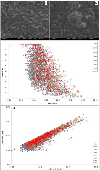
Figure 2.
Scanning electron microscopy images at different magnitudes (a,b) of representative samples; these show grain morphology. (c) Circularity vs. area and (d) minor vs. major axis length of the particles show the homogeneity of the samples. The area; circularity C, where C = 4π area/perimeter2 [48]; and major and minor axes of the best-fitting ellipse of the particles were determined on binary images extracted from photos with a 400 × 400-pixel resolution. The average aspect ratio (AR) is 1.70.
3.3. Mud Chemical Analysis
The mud geochemical analysis was carried out after air-drying, sifting (<2 mm), and quartering to obtain a representative sediment volume (about 200 gr). Soil chemical analysis followed the standard analytical procedure endorsed by the Italian Ministry of Agriculture (D.M. 13 September 1999 that ended on 25 March 2002). The mud conductivity and the pH were determined by an aqueous phase analysis after appropriate mixing with milliQ water. Mud acidity was measured either in water (pHw) or in calcium chloride (pHCa). The pHCa is considered the more accurate of the pH measured on the water as it reflects what the plant experiences in the sediment. The values of pHCa are usually lower than pHw by 0.5 to 0.9 following a nonlinear relationship. The pHCa was determined on a solution suspension of sediment–CaCl2 (0.1%) (1:2.5 ratio). The electrical conductivity was measured on a filtered (2.5 µm) aqueous extract of mud (1:2 sediment–water ratio) equilibrated overnight.
Major elements were determined on filtered (2.5 µm) aqueous extract of mud (1:5 sediment–water ratio). The alkalinity (HCO3− and CO32−) was not directly quantified by titration with 0.05 N HCl due to the turbidity of the samples. It was computed for difference among major anions and cations by assuming a maximum analytical error of 5%. Major elements were analyzed in the laboratory using chromatography systems (Dionex-Thermo ICS 1100) in suppressed mode, equipped with an anion column (AS14A) and a precolumn (AG14A) that works under a continuous flow of the carbonate–bicarbonate eluent for anions (F−, Cl−, Br−, NO3−, and SO42−) and a cation column (CS12A) and precolumn (CG12A) that works under a continuous flow of methanesulfonic acid for cations (Na+, K+, Mg2+, and Ca2+); the precision and accuracy of the method are described in [49]. Major anions and cations were determined on filtered (0.45 µm) and filtered and acidified (HCL 6M) samples, respectively. Chemical–physical parameters and major element chemistry of the sampled sediments are reported in Table 2.
Table 2.
Chemical–physical parameters and chemical composition of analyzed sediments.
3.4. Rheology
The rheological parameters, namely, the Bingham yield stress and the viscosity, were determined using an Anton Paar Physica MCR 301 rheometer equipped with an air-bearing system. A vane rotor system ST22-6V-16—with 6 vanes of 22 mm diameter and 16 mm length immersed in a cylindrical cup (CC27; 27 mm in diameter) [50,51]—was used for fluid suspensions (AM1, AM2, AM4, AM5, AM6, and AM7), and a parallel plate system (PP25; diameter of 25 mm and a distance between the 2 plates of 1.7 mm for AM3) was used for very viscous suspensions. The particular advantages of the vane geometry are its simplicity of fabrication, ease of cleaning, and, more than anything else, its elimination of serious wall slip effects. These geometric characteristics are very useful for the measurement of the flow properties of non-Newtonian liquids.
We used the rheometer in rotational mode for all 7 suspensions. The flow curves of all suspensions were carried out using the controlled shear stress (CSS) method: Steps of constant stresses were applied long enough to reach a steady apparent viscosity with time. For each step of stress, the steady state of viscosity and shear rate was reached [52]. The values of apparent viscosity and the shear rate were calculated by averaging their values reached at steady state for each stress step. Therefore, we could achieve the flow curves with shear stress and shear rate and with apparent viscosity and shear rate for all suspensions.
A fluid-saturated sand can liquefy in response to a sudden shock or earthquake under a shear rate that can be approximated by peak ground velocity (hereafter PGV) using the empirical relationship [53]. Using spectral velocity (vs) expected values of 800 and 1800 m/s [38] for the source area of the collected sample, we calculated that the studied materials underwent a shear rate between 3.4·10−5 and 7.8·10−3 s−1. This range of is within the shear rate obtained under the experimentally applied shear rate (10−3–10−7 s−1).
4. Results
4.1. Mud Chemistry
The electrical conductivity (EC) of the analyzed muds ranges from 1.61 to 3.52 mS/cm, corresponding to non-saline (0 < 2 ms/cm) and very slightly saline (2 < 4 mS/cm) muds (U.S. Salinity Laboratory Staff [54]). The highest EC value was measured in the ML3-A sample, whereas ML1-A had the lowest salt content.
The measured pHCa values are from 7.8 to 8.3, revealing neutral to weakly alkaline muds. In alkaline soils, pH is generally controlled by carbonate, often related to sodium. In the analyzed muds, the major ions are Na+ and alkalinity, showing a correlation trend despite a Na/alkalinity ratio of >1. Only sample ML1-A has a stoichiometric Na-HCO3 composition.
The sulfates show high variability, from 5.81 to 13.42 meq/L. The highest SO42− concentration belongs to sample ML3-A, which also has the highest EC. The analyzed mud samples are depleted in Ca2+ and Mg+2, maybe due to phosphate precipitation processes typical of alkaline sediments. The nitrate concentrations are generally low, excluding anthropogenic pollution, except for samples 3 and SV1-A, which have relatively high NO3− values, around 0.8 meq/L.
The fluorine content of the muds is relatively high, ranging from 0.061 meq/L (sample 1) to 0.326 meq/L (sample ML3-A). The natural fluorine concentration is generally high in mud, since it is directly related to the clay content [55]. However, contamination with fluorine-bearing phosphorous fertilizers could also enhance this element’s presence in soils.
The chlorides are generally low (from 0.21 to 1.57 meq/L), and bromides are below the detection limit in all the samples. The low salinity and low Cl− and Br− concentrations hint at a continental origin of the muds.
The high Na+ values and the depletion of Ca2+ and Mg2+ suggest cationic exchange processes mainly involving Na+-bearing minerals and Ca-rich waters. Another Na+ source could be due to the alkali feldspars weathering, recognized in SEM-EDS analyses.
The wide range of SO42− concentrations may be due to one or more sources for this ionic species, such as: (1) the leaching and dissolution of Messinian gypsum evaporitic horizons, present in the Colombacci and Laga formations (e.g., [38]) and (2) the contribution of fertilizer-polluted waters associated with moderate-to-high levels of nitrate, as occurring for sample 3.
According to the literature, shale formations are suitable for mud volcano formation, favored by a combination of gravitative instability of shales and fluid overpressures, e.g., Kopf [16] and Mazzini and Etiope [15]. Fluid overpressures can develop in the shale formation or in surrounding sedimentary rocks.
The low salinity of the analyzed muds suggests a continental origin, consistent with the Colombacci Formation rather than the Argille Azzurre Formation. The Colombacci Formation includes evaporite horizons, mainly gypsum, which could explain the high SO42− concentrations in water extracted from the muds. The semi-quantitative SEM-EDS analyses of the muds are compatible with the Colombacci origin since they recorded the presence of quartz, Fe-rich mica, alkali feldspars, carbonates, and clay minerals.
The geochemical analyses of mud volcanoes extruded from the Argille Azzurre formation at Salse di Nirano (Modena province, Italy) show higher EC values, ranging from 2.72 to 26.60 mS/cm and a Na-Cl composition typical of marine sediments [23].
4.2. Rheological Behavior
The measured rheological parameters were fitted using the Bingham model. The shear stress is given as a linear function of the shear rate and the constant material parameter yield stress and the Bingham viscosity:
where τ is the applied shear stress expressed in Pa, τb is the constant parameter yield stress expressed in Pa, η is the Bingham viscosity expressed in Pa·s, and is the shear rate expressed in s−1. Table 3 reports the rheological parameters determined for each suspension fitting the data with the Bingham model.
Table 3.
Rheological parameters determined for each suspension.
The Bingham viscosities of the mud suspension (Figure 3a) decrease from 6.3E+7 Pa∙s (AM6) to 6.9E+5 Pa∙s (AM7) with increasing water content from 13.5 to 29.5 wt.%.
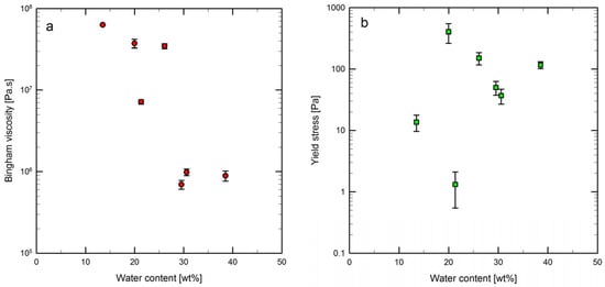
Figure 3.
Bingham viscosity (a) decreases with increasing water content of the liquefied muds. Yield stress (b) tendency with water content.
The yield stress τb, i.e., the stress that has to be exceeded to start the flow, is between 1 and 404 Pa (Figure 3b). Sample AM1 (30.5 wt.% of water), AM2 (26.1 wt.% of water), AM3 (19.9 wt.% of water), and AM7 (29.5 wt.% of water) show a reasonably linear decreasing yield stress, from 404 to 36.8 Pa, with increasing water content. The exceptions are samples AM5 (38.5 wt.% of water), AM3 (19.9 wt.% of water), and AM2 (26.1 wt.% of water) which have a high Bingham yield stress oscillating between 1.3 and 115.8 Pa.
Notably, the rheological parameters of the seven experimentally tested suspensions, with few exceptions, show an expected decrease in viscosity and yield stress as the amount of water increases.
5. Discussion
A few days after the Norcia earthquake, a sampling of mud emissions was performed at 7 sites in the area of Santa Vittoria in Matenano (SV emission point) and Monteleone di Fermo (ML emission point), which are located at 38 and 44 km, respectively, from the epicenter of the 30 October 2016 Mw 6.5 Norcia earthquake, Italy. At Monteleone di Fermo, 2 emission points (1 and 3) were reactivated. The fluids feeding the mud emission points SV and ML originated in the Laga flysch formation, a complex with generally low permeability but hosting locally perched aquifers stored in the highly permeable sandstone horizons [6,7].
The shock passage of seismic waves during the earthquake induced the disruptions of the sediment and the associated liquefaction in the presence of water.
Modeling Mudflow
We used two equations to model the flow from the emission points: the Jolly and Lonergan model [56] to calculate the rise velocity of liquefied muds and the Kaitna et al. model [57] to calculate the flow velocity on the substratum. In their study of sandstone intrusions due to seismicity-induced liquefaction, Jolly and Lonergan [56] found that the forceful intrusion of remobilized clastic sediment, and its emplacement into the surrounding strata, forms sheets of sediment that are discordant to bedding (dykes) or concordant with bedding (sills). These intrusions can stay in the substrate as fissures, dykes, and sills and can reach the surface as sand volcanoes and flow on the substratum. The injection of high-pressure fluids (with entrained sand grains) into the surrounding sediments requires a sustained pressure differential between the fluid in the propagating fracture or intrusion and the fluid in the pores of the sediment or sedimentary rock, so that the fracture dilates and the sand–fluid mixture can flow through the fracture as liquefied in response to a sudden shock, e.g., an earthquake [56]. We used the minimum fluidization velocity (Umf) proposed by Jolly and Lonergan ([56] and references therein):
where d is the grain diameter, ρf is the density of the fluid, ρs is the density of the grains, g is the acceleration due to gravity, and η the dynamic viscosity of the fluid (water; 3∙10−4 Pa∙s). We considered grains with a minimum and maximum size of 2 and 8 μm, respectively, based on the results of the granulometric analysis. ρf is the water density, and ρs was assumed equal to 1600 kg/m3. The result shows a minimum fluidization velocity ranging between 0.05 and 0.74 m/s for grain sizes of 2 and 8 μm, respectively.
By selecting the parameters listed in Table 3, and assuming a Bingham fluid moving on an infinitely wide plane, we determined the velocity V of the selected suspensions by applying the following relation [57]:
where ρ is the density of the mixtures—we used 1400 kg/m3, following Del Gaudio and Ventura [52], g is the gravity acceleration (9.8 m/s2), θ is the slope angle (we considered 2°, 5°, and 10°), η the dynamic Bingham viscosity, and y0 the thickness of the shear layer calculated as:
where H is the flow thickness (here assumed as 0.7 m). This relation holds for H ≥ y ≥ y0 (y is measured from the surface in its perpendicular direction) and can be used to determine the velocity of non-Newtonian suspensions provided that the thickness H, the density of the water, the suspended load, and the slope angle of the substratum are known. The results are summarized in Figure 4. The highest velocities are reached for sample AM7 (29.5 wt.% of water). If the AM7 flow moves on a substratum with a slope of 2°, the maximum velocity is 0.12 mm/s; if 5°, the maximum velocity is 0.37 mm/s; and if 10°, the maximum velocity is 0.79 mm/s. In the range of 10–30 wt.% of water content, the flow velocity increases with increasing water content. By increasing the water content of the sample above 30 wt.%, the velocity does not increase. This could reflect the lack of particle aggregates within the water–solid mixture and the consequent movement of the flow as a particle-free water stream.
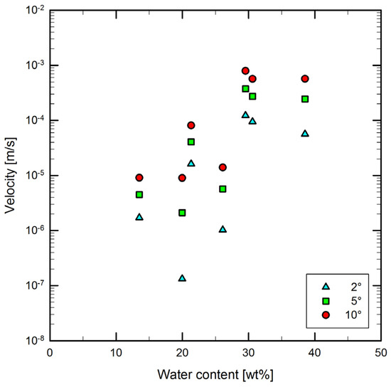
Figure 4.
Flow velocities [57] on substrates with different slope angles of 2°, 5°, and 10°.
6. Conclusions
The rheological behavior of muddy samples collected in the Fermo area after the Norcia earthquake on 30 October 2016 is consistent with that of a Bingham fluid. The same behavior was found by Mazzini et al. [30]; they studied the mudflow of Lusi volcanoes in Indonesia as a Bingham fluid with yield stress; conversely, Coussot and Piau [58] performed viscosity experiments on mud suspensions and found these to have shear-thinning rheology.
The Bingham viscosity shows a typical behavior: it lowers when increasing the water of the suspensions (from 6.3∙107 to 6.9∙105 Pa∙s). The Bingham yield stress follows a more complex behavior.
Using the rheological parameters in the experiments, we determined the rise and flow velocity along a slope of the studied muds. This result assumes relevant importance for the hazard of spreading liquefied sands. The rise velocity of liquefied mud is strongly dependent on the grain size and the fluid’s rheological properties; this velocity ranges between 0.05 and 0.74 m/s for grain sizes of 2 and 8 μm, respectively. Water-rich mudflows move faster on a slope as the water content increases up to 30 wt.%. Above this value, the flow velocity remains constant due to the disaggregation of bonds among the solid particles in the mixture. At the same time, liquefied mudflows move faster on large-slope-angle surfaces.
The geochemical analysis of the muds shows low electrical conductivity, a pH slightly alkaline, and high Na+, alkalinity, and SO42− content, suggesting a cationic exchange process in clay and weathering of gypsum and alkali feldspars. The mud origin is continental, likely belonging to the Colombacci Formation.
Author Contributions
Conceptualization, G.V., P.D.G. and V.M.; methodology, P.D.G., V.M., B.C., M.L. and A.S.; software, P.D.G. and V.M.; validation, P.D.G., V.M., B.C., A.S., M.L., S.A., D.D.N., P.M., T.R. and G.V.; formal analysis, V.M., B.C., P.D.G., A.S. and M.L.; investigation, P.D.G., T.R., S.A., D.D.N., A.S., B.C. and P.M.; resources, G.V.; data curation, P.D.G., V.M. and B.C.; writing—original draft preparation, P.D.G.; writing—review and editing, P.D.G., V.M., B.C., T.R. and A.S.; visualization, G.V.; supervision, G.V. All authors have read and agreed to the published version of the manuscript.
Funding
This research has been carried out with a funding of DPC-INGV.
Institutional Review Board Statement
Not applicable.
Informed Consent Statement
Not applicable.
Data Availability Statement
The data are only available in the tables in this article.
Acknowledgments
We thank the editor and two anonymous reviewers for comments and suggestions that allowed us to significantly improve the manuscript. We thank the INGV–EMERGEO Working Group (https://emergeo.ingv.it accessed on 2 June 2023) for the logistical and technical support during the field activities (project administration and funding acquisition) and the Mayor of Monteleone di Fermo, M. Fabiani, for his courtesy and support during the field campaign. We thank the HP–HT group of INGV for their support in the laboratory.
Conflicts of Interest
The authors declare no conflict of interest.
References
- Livio, F.; Michetti, A.M.; Vittori, E.; Gregory, L.; Wedmore, L.; Piccardi, L. Central Italy earthquake working group. Surface faulting during the August 24, 2016, central Italy earthquake (Mw = 6.0): Preliminary results. Ann. Geophys. 2016, 59, 1–8. [Google Scholar]
- Tinti, E.; Scognamiglio, L.; Michelini, A.; Cocco, M. Slip heterogeneity and directivity of the ML 6.0, 2016, Amatrice earthquake estimated with rapid finite-fault inversion. Geophys. Res. Lett. 2016, 43, 10745–10752. [Google Scholar] [CrossRef]
- Chiaraluce, L.; Di Stefano, R.; Tinti, E.; Scognamiglio, L.; Michele, M.; Casarotti, E.; Lombardi, A. The 2016 Central Italy seismic sequence: A first look at the mainshocks, aftershocks, and source models. Seismol. Res. Lett. 2017, 88, 757–771. [Google Scholar] [CrossRef]
- Cheloni, D.; De Novellis, V.; Albano, M.; Antonioli, A.; Anzidei, M.; Atzori, S.; Doglioni, C. Geodetic model of the 2016 Central Italy seismic sequence: A first look at the mainshocks, aftershocks, and source models. Seismol. Res. Lett. 2017, 88, 757–771. [Google Scholar]
- Pucci, S.; De Martini, P.M.; Civico, R.; Villani, F.; Nappi, R.; Ricci, T.; Azzaro, R.; Brunori, C.A.; Caciagli, M.; Cinti, F.R.; et al. Coseismic ruptures of the 24 August 2016, Mw 6.0 Amatrice earthquake (central Italy). Geophys. Res. Lett. 2017, 44, 2138–2147. [Google Scholar] [CrossRef]
- Civico, R.; Pucci, S.; Villani, F.; Pizzimenti, L.; De Martini, P.M.; Nappi, R.; the Open EMERGEO Working Group. Surface ruptures following the 30 October 2016 Mw 6.5 Norcia earthquake, central Italy. J. Maps 2018, 14, 151–160. [Google Scholar] [CrossRef]
- Villani, F.; Civico, R.; Pucci, S.; Pizzimenti, L.; Nappi, R.; De Martini, P.M.; the Open EMERGEO Working Group. A database of the post-30 October 2016 Norcia earthquake coseismic effects in Central Italy, Scientific Data. Nature 2018, 5, 180049. [Google Scholar] [CrossRef]
- Improta, L.; Latorre, D.; Margheriti, L.; Nardi, A.; Marchetti, A.; Lombardi, A.M.; Castello, B.; Villani, F.; Ciaccio, M.G.; Mele, F.M.; et al. Multi-segment rupture of the 2016 Amatrice-Visso-Norcia seismic sequence (central Italy) constrained by the first high-quality catalog of Early Aftershocks. Sci. Rep. 2019, 9, 6921. [Google Scholar] [CrossRef]
- Moschella, M.; Ciaccio, M.G.; Latorre, D. Minor earthquake sequences in the Amatrice-Norcia epicentral area (Central Italy). Tectonophysics 2021, 809, 228858. [Google Scholar] [CrossRef]
- Ojeda, J.; Akinci, A.; Tinti, E.; Arriola, S.; Ruiz, S. Hybrid broadband strong-motion simulation to investigate the near-source characteristics of the M6.5, 30 October 2016 Norcia, Italy earthquake. Soil Dyn. Earthq. Eng. 2021, 149, 106866. [Google Scholar] [CrossRef]
- Maslovaric, G.; Zaccagnino, M.; Mezzaluna, C.; Perilli, S.; Trivellato, D.; Longo, V.; Civilotti, C. The Effectiveness of Eye Movement Desensitization and Reprocessing Integrative Group Protocol with Adolescent Survivors of the Central Italy Earthquake. Front. Phychol. Sec. Phychol. Clin. Settings 2017, 8, 1826. [Google Scholar] [CrossRef] [PubMed]
- Farabollini, P.; Angelini, S.; Fazzini, M.; Lugeri, F.R.; Scalella, G.; GeomorphoLab. Earthquakes and Society: The 2016 central Italy reverse seismic sequence. In Earthquake Risk Perception, Communication and Mitigation Strategies across Europe; Geographies of the Anthropocene (Il Sileno Edizioni); Farabollini, P., Lugeri, F.R., Mugnano, S., Eds.; Il Sileno Edizioni: Lago, Italy, 2019; Volume 2, pp. 249–266. ISSN 2611-3171. Available online: http://www.ilsileno.it/geographiesoftheanthropocene/e-book-releases/ (accessed on 2 June 2023).
- EMERGEO Working Group. A new photographic dataset of the coseismic geological effects originated by the Mw 5.9 Visso and Mw 6.5 Norcia earthquakes (26th and 30th October 2016, central Italy). Misc. INGV 2017, 38, 1–114. [Google Scholar]
- Martinelli, G.; Judd, A. Mud volcanoes of Italy. Geol. J. 2004, 39, 49–61. [Google Scholar] [CrossRef]
- Mazzini, A.; Etiope, G. Mud volcanism: An updated review. Earth-Sci. Rev. 2017, 168, 81–112. [Google Scholar] [CrossRef]
- Kopf, A.J. Significance of mud volcanism. Rev. Geophys. 2002, 40, 1005. [Google Scholar] [CrossRef]
- Planke, S.; Svensen, H.; Hovland, M.; Banks, D.A.; Jamtveit, B. Mud and fluid migration in active mud volcanoes in Azerbaijan. Geo-Mar. Lett. 2003, 23, 258–268. [Google Scholar] [CrossRef]
- Bonini, M. Elliptical mud volcano caldera as stress indicator in an active compressional setting (Nirano, Pede-Apennine margin. northern Italy). Geology 2008, 36, 131–134. [Google Scholar] [CrossRef]
- Capozzi, R.; Picotti, V. Fluid migration and origin of a mud volcano in the Northern Apennine (Italy): The role of deeply rooted normal faults. Terra Nova 2002, 14, 363–370. [Google Scholar] [CrossRef]
- Capozzi, R.; Picotti, V. Spontaneous fluid emissions in the Northern Apennines: Geochemistry, structures and implications for the petroleum system. Geol. Soc. Lond. Spec. Publ. 2010, 348, 115–135. [Google Scholar] [CrossRef]
- Lupi, M.; Ricci, B.S.; Kenkel, J.; Ricci, T.; Fuchs, F.; Miller, S.A.; Kemna, A. Subsurface fluid distribution and possible seismic precursory signal at the Salse di Nirano mud volcanic field, Italy. Geophys. J. Int. 2015, 204, 907–917. [Google Scholar] [CrossRef]
- Oppo, D.; Capozzi, R.; Picotti, V. A new model of the petroleum system in the Northern Apennines, Italy. Mar. Pet. Geol. 2013, 48, 57–76. [Google Scholar] [CrossRef]
- Sciarra, A.; Cantucci, B.; Ricci, T.; Tomonaga, Y.; Mazzini, A. Geochemical characterization of the Nirano mud volcano, Italy. Appl. Geochem. 2019, 102, 77–87. [Google Scholar] [CrossRef]
- Bonasera, F. I vulcanelli di fango del Preappennino Marchigiano. Riv. Geogr. Ital. 1952, 59, 16–26. [Google Scholar]
- Bonasera, F. I vulcanelli di fango dell’Abruzzo orientale. Riv. Geogr. Ital. 1954, 61, 217–223. [Google Scholar]
- Damiani, A.V. Studio della Salsa di Offida (Ascoli Piceno, Marche). L’Universo 1964, 3, 473–487. [Google Scholar]
- Etiope, G.; Martinelli, G. ‘‘Pieve Santo Stefano’’ is not a mud volcano: Comment on ‘‘Structural controls on a carbon dioxide-driven mud volcano field in the Northern Apennines’’ (by Bonini, 2009). J. Struct. Geol. 2009, 31, 1270–1271. [Google Scholar] [CrossRef]
- Etiope, G.; Milkov, A.V. A new estimate of global methane flux from onshore and shallow submarine mud volcanoes to the atmosphere. Environ. Geol. 2004, 46, 997–1002. [Google Scholar] [CrossRef]
- Etiope, G. Natural gas seepage. In Earth’s Hydrocarbon Degassing; Springer: Berlin/Heidelberg, Germany, 2015. [Google Scholar] [CrossRef]
- Mazzini, A.; Nermoen, A.; Krotkiewski, M.; Podladchikov, Y.; Planke, S.; Svensen, H. Strike-slip faulting as a trigger mechanism for overpressure release through piercement. Mar. Pet. Geol. 2009, 26, 1751–1765. [Google Scholar] [CrossRef]
- Hedberg, H.D. Relation of methane generation to undercompacted shales, sale diapirs, and mud volcanoes. AAPG Bull. 1974, 58, 661–673. [Google Scholar]
- Reed, D.L.; Silver, E.A.; Tagudin, J.E.; Shipley, T.H.; Vrolijk, P. Relations between mud volcanoes, thrust deformation, slope sedimentation, and gas hydrate, offshore north Panama. Mar. Pet. Geol. 1990, 7, 44–54. [Google Scholar] [CrossRef]
- Kopf, A.J. Making calderas from mud. Nat. Geosci. 2008, 1, 500–501. [Google Scholar] [CrossRef]
- Lynch, D.K.; Hudnut, K.W. The Wister mud pot lineament: Southeastward extension or abandoned strand of the San Andreas fault? Bull. Seismol. Soc. Am. 2008, 98, 1720–1729. [Google Scholar] [CrossRef]
- Manga, M.; Brumm, M.; Rudolph, M.L. Earthquake triggering of mud Volcanoes. Mar. Pet. Geol. 2009, 26, 1785–1798. [Google Scholar] [CrossRef]
- Hanotinm, C.; Kiesgen de Richterm, S.; Marchalm, P.; Michotm, L.J.; Baravianm, C. Vibration-induced Liquefaction of Granular Suspensions. Phys. Rev. Lett. 2012, 108, 198301. [Google Scholar] [CrossRef] [PubMed]
- Lanzo, G.; Tommasi, P.; Ausilio, E.; Aversa, S.; Bozzoni, F.; Cairo, R.; d’Onofrio, A.; Durante, M.G.; Foti, S.; Giallini, S.; et al. Reconnaissance of geotechnical aspects of the 2016 Central Italy earthquakes. Bull. Earthq. Eng. 2019, 17, 5495–5532. [Google Scholar] [CrossRef]
- Maestrelli, D.; Bonini, M.; Delle Donne, D.; Manga, M.; Piccardi, L.; Sani, F. Dynamic triggering of mud volcano eruptions during the 2016–2017 Central Italy seismic sequence. J. Geophys. Res. Solid Earth 2017, 122, 9149–9165. [Google Scholar] [CrossRef]
- Bigi, S.; Calamita, F.; Cello, G.; Centamore, E.; Deiana, G.; Paltrinieri, W.; Ridolfi, M. Tectonics and sedimentation within a Messinian foredeep in the Central Apennines, Italy. J. Pet. Geol. 1999, 22, 5–18. [Google Scholar] [CrossRef]
- Centamore, E.; Cantalamessa, G.; Micarelli, A.; Potetti, M.; Berti, D.; Bigi, S.; Ridolfi, M. Stratigrafia e analisi di facies dei depositi del Miocene e del Pliocene inferiore dell’avanfossa marchigiano-abruzzese e delle zone limitrofe. Studi Geol. Camerti 1991, 2, 125–131. [Google Scholar]
- Carafa, M.M.C.; Galvani, A.; Di Naccio, D.; Kastelic, V.; Di Lorenzo, C.; Miccolis, S.; Sepe, V.; Pietrantonio, G.; Gizzi, C.; Massucci, A.; et al. Partitioning the ongoing extension of the central Apennines (Italy): Fault slip rates and bulk deformation rates from geodetic and stress data. J. Geophys. Res. Solid Earth 2020, 125, e2019JB018956. [Google Scholar] [CrossRef]
- Boncio, P.; Lavecchia, G.; Milana, G.; Rozzi, B. Seismogenesis in Central Apennines, Italy: An integrated analysis of minor earthquake sequences and structural data in the Amatrice-Campotosto area. Ann. Geophys. 2004, 47, 1723–1742. [Google Scholar] [CrossRef]
- Galadini, F.; Galli, P. Active tectonics in the Central Apennines (Italy)—Input data for Seismic Hazard Assessment. Nat. Hazards 2000, 22, 225–270. [Google Scholar] [CrossRef]
- Lavecchia, G.; Ferrarini, F.; Brozzetti, F.; De Nardis, R.; Boncio, P.; Chiaraluce, L. From surface geology to aftershock analysis: Constraints on the geometry of the L’Aquila 2009 seismogenic fault system. Ital. J. Geosci. (Boll. Soc. Geol. Ital.) 2012, 131, 330–347. [Google Scholar] [CrossRef]
- Galadini, F.; Galli, P.; Leschiutta, I.; Monachesi, G.; Stucchi, M. Active tectonics and seismicity in the area of the 1997 earthquake sequence in Central Italy: A. short review. J. Seismol. 1999, 3, 165–175. [Google Scholar] [CrossRef]
- Rovida, A.; Locati, M.; Camassi, R.; Lolli, B.; Gasperini, P. (Eds.) CPTI15, the 2015 Version of the Parametric Catalogue of Italian Earthquakes; Istituto Nazionale di Geofisica e Vulcanologia: Bologna, Italy, 2016. [Google Scholar] [CrossRef]
- Chiaraluce, L. Unravelling the complexity of Apenninic extensional fault systems: A review of the 2009 L’Aquila earthquake (Central Apennines, Italy). J. Struct. Geol. 2012, 42, 2–18. [Google Scholar] [CrossRef]
- Cox, M.R.; Budhu, B.A. practical approach to grain shape quantification. Eng. Geol. 2008, 96, 1–16. [Google Scholar] [CrossRef]
- Prano, V.; Liotta, M. Precisione e accuratezza nella determinazione dei costituenti maggiori in soluzione acquosa mediante cromatografia ionica: Stime per i cromatografi Dionex ICS-1100 utilizzati presso la Sezione INGV di Palermo. Rapp. Tec. INGV 2017, 390, 1–22. [Google Scholar] [CrossRef]
- Barnesm, H.A.; Nguyenm, Q.D. Rotating vane rheometry—A review. J. Non-Newton. Fluid Mech. 2001, 98, 1–14. [Google Scholar] [CrossRef]
- Scotto di Santolo, A.; Pellegrino, A.M.; Evangelista, A. Experimental study on the rheological behavior of debris flow. Nat. Hazards Earth Syst. Sci. 2010, 10, 2507–2514. [Google Scholar] [CrossRef]
- Del Gaudio, P.; Ventura, G. Flow Behavior of Clay-Silt to Sand-Silt Water-Rich Suspensions at Low to High Shear Rates: Implications for Slurries, Transitional Flows, and Submarine Debris-Flows. Acta Geol. Sin. 2018, 92, 2395–2404. [Google Scholar] [CrossRef]
- Rudolph, M.L.; Manga, M. Mud volcano response to the 4 April 2010 El Mayor-Cucapah earthquake. J. Geophys. Res. 2010, 115, B12211. [Google Scholar] [CrossRef]
- U.S. Salinity Laboratory Staff. Diagnosis and improvement of saline and alkali soils. In US Department of Agriculture Handbook 60; U.S. Salinity Laboratory Staff: Washington, DC, USA, 1954. [Google Scholar]
- Bombik, E.; Bombik, A.; Górski, K.; Saba, L.; Bombik, T.; Rymuza, K. The Effect of Environmental Contamination by Fluorine Compounds on Selected Horse Tissues. Pol. J. Environ. Stud. 2011, 20, 37–43. [Google Scholar]
- Jolly, R.J.H.; Lonergan, L. Mechanisms and controls on the formation of sand intrusions. J. Geol. Soc. Lond. 2002, 159, 605–617. [Google Scholar] [CrossRef]
- Kaitna, R.; Rickenmann, D.; Schatzmann, M. Experimental study on rheological behaviour of debris flow material. Acta Geotech. 2007, 2, 71–85. [Google Scholar] [CrossRef]
- Coussotm, P.; Piaum, J.M. On the behavior of fine mud suspensions. Rheol. Acta 1994, 33, 175–184. [Google Scholar] [CrossRef]


Disclaimer/Publisher’s Note: The statements, opinions and data contained in all publications are solely those of the individual author(s) and contributor(s) and not of MDPI and/or the editor(s). MDPI and/or the editor(s) disclaim responsibility for any injury to people or property resulting from any ideas, methods, instructions or products referred to in the content. |
© 2023 by the authors. Licensee MDPI, Basel, Switzerland. This article is an open access article distributed under the terms and conditions of the Creative Commons Attribution (CC BY) license (https://creativecommons.org/licenses/by/4.0/).