A Solution Procedure to Improve 3D Solid Finite Element Analysis with an Enrichment Scheme

Abstract

This paper presents a novel and efficient solution procedure to improve 3D solid finite element analysis with an enrichment scheme. To this end, we employ finite elements enriched by polynomial cover functions, which can expand their solution space without requiring mesh refinement or additional nodes. To facilitate this solution procedure, an error estimation method and cover function selection scheme for 3D solid finite element analysis are developed. This enables the identification of nodes with suboptimal solution accuracy, allowing for the adaptive application of cover functions in a systematic and efficient manner. Furthermore, a significant advantage of this procedure is its consistency, achieved by excluding arbitrary coefficients from the formulations employed. The effectiveness of the proposed procedure is demonstrated through several numerical examples. In the majority of the examples, it is observed that the stress prediction error is reduced by more than half after applying the proposed procedure.

1. Introduction

During the last decades, the finite element method (FEM) has been widely used for analyzing various engineering problems and still many researchers have been devoted to improving the accuracy of solutions [1,2,3,4]. Despite its notable success, the standard finite element method (ST-FEM) has some drawbacks, especially in solution accuracy which is affected by the finite element mesh and the use of linear elements such as 2D 3-node triangular and 3D 4-node tetrahedral elements that have considerably low accuracy in stress and strain prediction [5,6,7]. There are several ways to improve the accuracy, such as increasing mesh density and adding nodes to use higher-order finite elements.

In addition, numerous studies have been carried out to overcome these limitations of the standard FEM (ST-FEM). As a result, several numerical methods have been developed, including extended FEM (EX-FEM), enriched FEM (EN-FEM), and smoothed FEM (S-FEM) [6,7,8,9,10]. EX- and EN-FEM improve the solution accuracy by supplementing their solution space [11,12,13]. S-FEM improves the accuracy by using information from neighboring elements [14,15,16,17].

Among numerical methods, an enrichment scheme expands the solution space by introducing cover functions to additional degrees of freedom (DOFs) compared to the standard DOFs of ST-FEM [18,19]. It can enhance finite element analysis solution like the p-version of the ST-FEM but does not require additional nodes. Also, different cover functions can be applied to each node. Therefore, the solution accuracy of the finite element analysis result could be effectively improved through adaptively applying the cover function to the local region where the predictive capability needs to be improved. [19]. However, the presence of linear dependence (LD) problems has limited the use of enriched finite elements. When the LD problem occurs, it is difficult to obtain reliable solutions because the stiffness matrix becomes a singular matrix.

Various approaches have been proposed to address the LD problem in EN-FEM [20,21,22], and effective ways to avoid the LD problem have been suggested in recent studies [23,24,25]. One such solution proposed by Tian involves suppressing all degrees of freedom corresponding to the cover function at the node where essential boundary conditions are imposed for 3-node triangular and 4-node tetrahedral elements [20]. Kim and Lee proposed the use of piecewise linear shape functions as the partition of unity functions for geometry and displacement interpolations to effectively resolve the LD problem for 4-node quadrilateral, 8-node hexahedral, 6-node prismatic, and 5-node pyramidal elements [23,24]. The feasibility of improving solution accuracy through the adaptive use of cover functions was also demonstrated in these studies [24].

Several studies have proposed procedures for the use of enriched finite elements to automatically enhance the accuracy of finite element solutions [19,25]. Kim and Bathe proposed a method for automatically applying cover functions based on the estimated error for each node, but their study was restricted to 2D and 3D linear elements and involved artificial coefficients [19]. Lee and Kim presented a procedure for enhancing the analysis accuracy in a 2D problem with a 2D 4-node quadrilateral element free from the LD problem. This study reduced the number of artificial coefficients compared to prior studies and demonstrated the feasibility of automatic accuracy improvement [25].

The aim of this paper is to propose a procedure that automatically enhances the accuracy of 3D solid finite element solutions using enriched 3D solid finite elements, including 4-node tetrahedral, 5-node pyramidal, 6-node prism, and 8-node hexahedral elements. The proposed procedure involves an error indicator that evaluates the error in finite element solutions for each node and a cover function selection scheme that applies cover functions to areas requiring improved solution accuracy based on the error indicator. This enrichment approach can enhance solution accuracy without requiring mesh refinement.

In the following sections, a brief review of the enriched 3D solid finite elements including 4-node tetrahedral, 5-node pyramidal, 6-node prism, and 8-node hexahedral elements with both linear and piecewise linear shape functions are provided. Then, we present a procedure for automatically selecting nodes to apply the cover functions to and determining the degree of cover functions to enhance the finite element solutions. Several numerical examples are provided to illustrate the effectiveness of the proposed procedure, and the paper concludes with a summary of the findings.

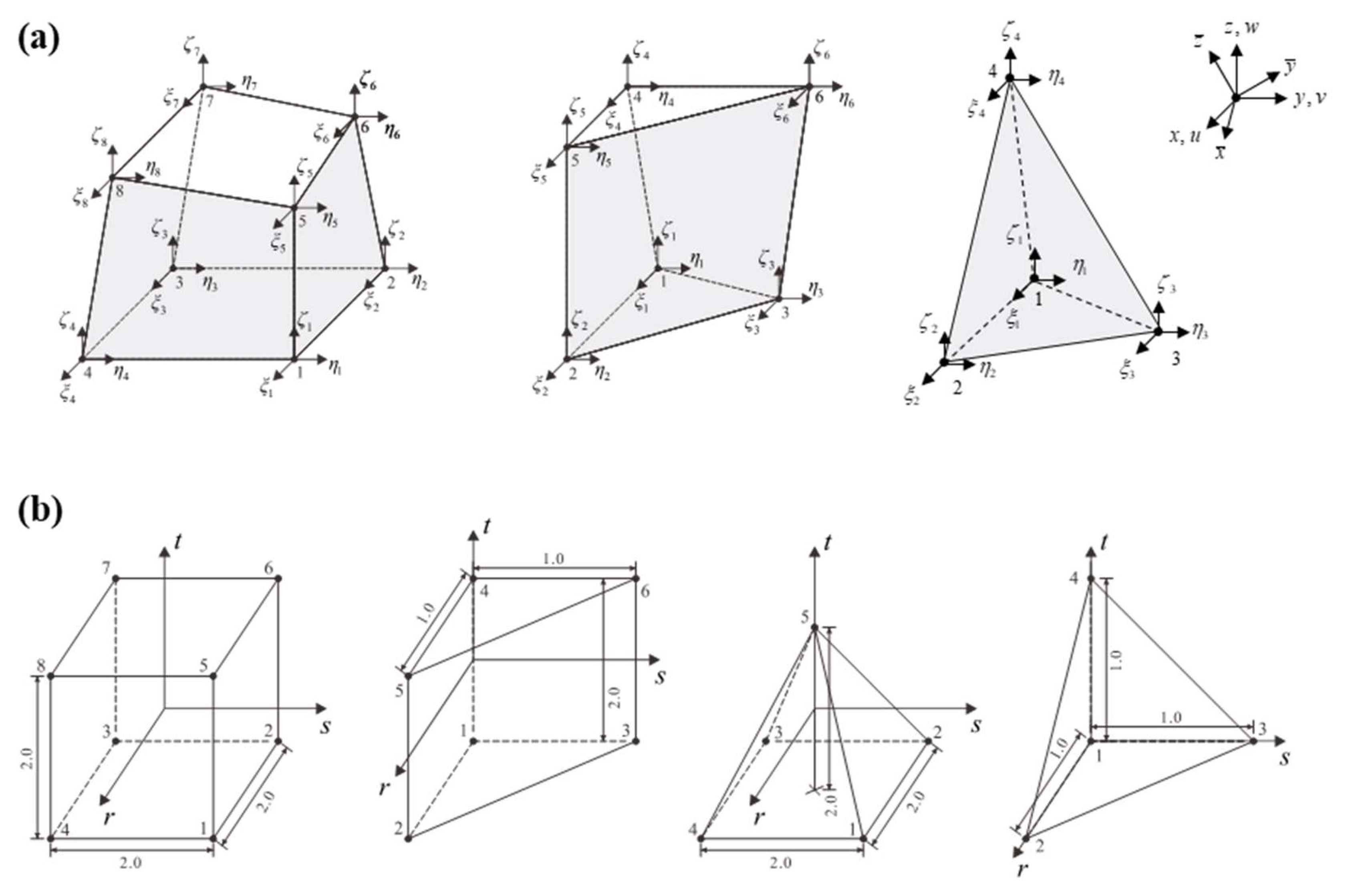
2. Finite Element Formulation Enriched by Cover Functions

In this section, we revisit the formulation of enriched 3D solid finite elements that has a well-established mathematical background and is free from the linear dependence problem [5,24]. Among 3D solid finite elements, we consider the 5-node pyramidal, 6-node prismatic, and 8-node hexahedral elements shown in Figure 1, which utilize a set of piecewise linear shape functions as the partition of the unity function for each element, and 4-node tetrahedral element based on the shape function of the standard finite element method.

For the piecewise linear shape function of the 5-node pyramidal, 6-node prismatic, and 8-node hexahedral element, each element is divided into several tetrahedral sub-domains using the set of points including $n$ nodes and $n_{quad}$ centers of the quadrilateral faces as shown in Figure 2.

Each set of points is assigned as the vertices of a tetrahedral sub-domain. A total of 24, 14, and 8 sub-domains are defined for the 5-node pyramidal, 6-node prismatic, and 8-node hexahedral elements, respectively [24]. Information on the tetrahedral sub-domain for each element is omitted for simplicity in this paper and can be found in Ref. [24]. Note that the 4-node tetrahedral element does not have a tetrahedral sub-domain.

For each tetrahedral sub-domain, the linear shape functions corresponding to node $i$ are given by

$$h_i^n=(a_i+b_{i}r+c_{i}s+d_{i}t)/n,$$

(1)

in which coefficients $a_i$, $b_i$, and $c_i$ for the piecewise linear shape functions are not included in this paper for the sake of simplicity, see Ref. [24] for detailed information, and $n$ is the number of nodes in the element.

The interpolation of geometry for the enriched 3D solid finite elements is given by

$$x(r,s,t)={\displaystyle \sum _{i=1}^n{h}_i^n(r,s,t)x_i} \mathrm{with} x_i={[\begin{array}{ccc}{x}_i& y_i& z_i\end{array}]}^{\mathrm{T}},$$

(2)

where the vector $x_i$ denotes the position of node i in the global Cartesian coordinate system in Figure 1a, n is the number of nodes, and $h_i(r,s,t)$ is the shape function corresponding to node i defined in the natural coordinate system in Figure 1b.

The interpolation of the displacement of the enriched 3D solid finite elements is obtained by multiplying the shape functions with the cover functions defined in cover area $C_i$ as follows [5,13]:

$$u(r,s,t)={\displaystyle \sum _{i=1}^n{h}_i^n(r,s,t){\tilde{u}}_i} \mathrm{with} {\tilde{u}}_i={[\begin{array}{ccc}{\tilde{u}}_i& {\tilde{v}}_i& {\tilde{w}}_i\end{array}]}^{\mathrm{T}},$$

(3)

where displacements ${\tilde{u}}_i$, ${\tilde{v}}_i$, and ${\tilde{w}}_i$ are cover functions in the x-, y- and z-directions, respectively, and the cover region $C_i$ is the union of elements attached to node i, as shown in Figure 3.

The cover functions are expressed as

$${\tilde{u}}_i=p_i(x)u_i^u, {\tilde{v}}_i=p_i(x)u_i^v, {\tilde{w}}_i=p_i(x)u_i^w \mathrm{in} C_i$$

(4)

with

$$\begin{array}{c}{p}_i(x)=[\begin{array}{ccccccccc}1& {\xi }_i& {\eta }_i& {\zeta }_i& {\xi }_i^2& {\xi }_i{\eta }_i& \cdots & {\xi }_i^d& \cdots \end{array}],\\ {\xi }_i=\frac{(x-x_i)}{{\chi }_i}, {\eta }_i=\frac{(y-y_i)}{{\chi }_i}, {\zeta }_i=\frac{(z-z_i)}{{\chi }_i},\\ u_i^u={[\begin{array}{ccccccccc}{u}_i^1& u_i^{\xi }& u_i^{\eta }& u_i^{\zeta }& u_i^{{\xi }^2}& u_i^{\xi \eta }& \cdots & u_i^{{\xi }^d}& \cdots \end{array}]}^{\mathrm{T}},\\ u_i^v={[\begin{array}{ccccccccc}{v}_i^1& v_i^{\xi }& v_i^{\eta }& v_i^{\zeta }& v_i^{{\xi }^2}& v_i^{\xi \eta }& \cdots & v_i^{{\xi }^d}& \cdots \end{array}]}^{\mathrm{T}},\\ u_i^w={[\begin{array}{ccccccccc}{w}_i^1& w_i^{\xi }& w_i^{\eta }& w_i^{\zeta }& w_i^{{\xi }^2}& w_i^{\xi \eta }& \cdots & w_i^{{\xi }^d}& \cdots \end{array}]}^{\mathrm{T}},\end{array}$$

(5)

in which $p(x)$ is a complete polynomial basis vector for node i, the vectors $u_i^u$, $u_i^v$, and $u_i^w$ are the degrees of freedom (DOFs) for the complete polynomial bases corresponding to the displacements $u$, $v$, and $w$, respectively, $d$ is the order of complete polynomial bases, and ${\chi }_i$ is the longest edge length of elements attached to node i.

By substituting (4) into (3), the interpolation of displacement for the enriched 3D solid elements is given by

$$u(r,s,t)={\displaystyle \sum _{i=1}^n{H}_i^n(r,s,t)u_i}$$

(6)

with

$$H_i^n(r,s,t)=\left[\begin{array}{ccc}{h}_i^n(r,s,t)& 0& 0\\ 0& h_i^n(r,s,t)& 0\\ 0& 0& h_i^n(r,s,t)\end{array}\right], h_i^n=h_i^n{p}_i, u_i=\left[\begin{array}{c}{u}_i^u\\ u_i^v\\ u_i^w\end{array}\right]$$

(7)

where $u_i$ and $H_i^n(r,s,t)$ are the nodal DOFs vector at node i and the corresponding interpolation matrix, respectively.

Using the strain-displacement relation, the strain vector in the global Cartesian coordinate system is expressed as [1,2,3]

$$\epsilon (r,s,t)={\left[\begin{array}{cccccc}{\epsilon }_{xx}& {\epsilon }_{yy}& {\epsilon }_{zz}& 2{\epsilon }_{xy}& 2{\epsilon }_{yz}& 2{\epsilon }_{zx}\end{array}\right]}^{\mathrm{T}}={\displaystyle \sum _{i=1}^n{B}_i^n(r,s,t)}{u}_i$$

(8)

where $B_i^n$ is the matrix for the relation between strain and displacement. In the local Cartesian coordinate system, the strain vector is given by

$$\overline{\epsilon }={\left[\begin{array}{cccccc}{\epsilon }_{\overline{x}\overline{x}}& {\epsilon }_{\overline{y}\overline{y}}& {\epsilon }_{\overline{z}\overline{z}}& 2{\epsilon }_{\overline{x}\overline{y}}& 2{\epsilon }_{\overline{y}\overline{z}}& 2{\epsilon }_{\overline{z}\overline{x}}\end{array}\right]}^{\mathrm{T}}={(T^{\epsilon })}^{-1}\epsilon ,$$

(9)

with

$$T^{\epsilon }=\left[\begin{array}{cccccc}{Q}_{x\overline{x}}^2& Q_{x\overline{y}}^2& Q_{x\overline{z}}^2& Q_{x\overline{x}}{Q}_{x\overline{y}}& Q_{x\overline{y}}{Q}_{x\overline{z}}& Q_{x\overline{z}}{Q}_{x\overline{x}}\\ Q_{y\overline{x}}^2& Q_{y\overline{y}}^2& Q_{y\overline{z}}^2& Q_{y\overline{x}}{Q}_{y\overline{y}}& Q_{y\overline{y}}{Q}_{y\overline{z}}& Q_{y\overline{z}}{Q}_{y\overline{x}}\\ Q_{z\overline{x}}^2& Q_{z\overline{y}}^2& Q_{z\overline{\underset{\_}{z}}}^2& Q_{z\overline{x}}{Q}_{z\overline{y}}& Q_{z\overline{y}}{Q}_{z\overline{z}}& Q_{z\overline{z}}{Q}_{z\overline{x}}\\ 2Q_{x\overline{x}}{Q}_{y\overline{x}}& 2Q_{x\overline{y}}{Q}_{y\overline{y}}& 2Q_{x\overline{z}}{Q}_{y\overline{z}}& Q_{x\overline{x}}{Q}_{y\overline{y}}+Q_{x\overline{y}}{Q}_{y\overline{x}}& Q_{x\overline{y}}{Q}_{y\overline{z}}+Q_{x\overline{z}}{Q}_{y\overline{y}}& Q_{x\overline{z}}{Q}_{y\overline{x}}+Q_{x\overline{x}}{Q}_{y\overline{z}}\\ 2Q_{y\overline{x}}{Q}_{z\overline{x}}& 2Q_{y\overline{y}}{Q}_{z\overline{y}}& 2Q_{y\overline{z}}{Q}_{z\overline{z}}& Q_{y\overline{x}}{Q}_{z\overline{y}}+Q_{y\overline{y}}{Q}_{z\overline{x}}& Q_{y\overline{y}}{Q}_{z\overline{z}}+Q_{y\overline{z}}{Q}_{z\overline{y}}& Q_{y\overline{z}}{Q}_{z\overline{x}}+Q_{y\overline{x}}{Q}_{z\overline{z}}\\ 2Q_{z\overline{x}}{Q}_{x\overline{x}}& 2Q_{z\overline{y}}{Q}_{x\overline{y}}& 2Q_{z\overline{z}}{Q}_{x\overline{z}}& Q_{z\overline{x}}{Q}_{x\overline{y}}+Q_{x\overline{y}}{Q}_{x\overline{x}}& Q_{z\overline{y}}{Q}_{x\overline{z}}+Q_{z\overline{z}}{Q}_{x\overline{y}}& Q_{z\overline{z}}{Q}_{x\overline{x}}+Q_{z\overline{x}}{Q}_{x\overline{z}}\end{array}\right],$$

(10)

in which $Q_{x\overline{y}}=e_x\cdot {\overline{e}}_y$ is the dot product of $e_x$ and ${\overline{e}}_y$. Here, $e_x$ and ${\overline{e}}_y$ are the unit vectors in the x-direction of the global Cartesian coordinate system and in the y-direction of the local Cartesian coordinate system, respectively. See Figure 1a.

For isotropic material, the stress vector in the global Cartesian coordinate system is written by

$$\sigma ={\left[\begin{array}{cccccc}{\sigma }_{xx}& {\sigma }_{yy}& {\sigma }_{zz}& {\sigma }_{xy}& {\sigma }_{yz}& {\sigma }_{zx}\end{array}\right]}^{\mathrm{T}}=C^{\mathrm{iso}}\epsilon ,$$

(11)

with

$$C^{\mathrm{iso}}=\frac{E}{(1+\nu )(1-2\nu )}\left[\begin{array}{cccccc}1-\nu & \nu & \nu & 0& 0& 0\\ \nu & 1-\nu & \nu & 0& 0& 0\\ \nu & \nu & 1-\nu & 0& 0& 0\\ 0& 0& 0& (1-2\nu )/2& 0& 0\\ 0& 0& 0& 0& (1-2\nu )/2& 0\\ 0& 0& 0& 0& 0& (1-2\nu )/2\end{array}\right],$$

(12)

where $E$ and $\nu$ are the elastic modulus and Poisson’s ratio, respectively. For orthotropic material, the stress vector in the local Cartesian coordinate system is given as

$$\overline{\sigma }={\left[\begin{array}{cccccc}{\sigma }_{\overline{x}\overline{x}}& {\sigma }_{\overline{y}\overline{y}}& {\sigma }_{\overline{z}\overline{z}}& {\sigma }_{\overline{x}\overline{y}}& {\sigma }_{\overline{y}\overline{z}}& {\sigma }_{\overline{z}\overline{x}}\end{array}\right]}^{\mathrm{T}}={\overline{C}}^{\mathrm{ortho}}\overline{\epsilon },$$

(13)

with

$${\overline{C}}^{\mathrm{ortho}}=\left[\begin{array}{cccccc}\frac{1-v_{\overline{y}\overline{z}}{v}_{\overline{z}\overline{y}}}{E_{\overline{x}}{E}_{\overline{y}}\mathrm{\Delta }}& \frac{{\nu }_{\overline{y}\overline{x}}+v_{\overline{y}\overline{z}}{v}_{\overline{z}\overline{x}}}{E_{\overline{y}}{E}_{\stackrel{⌢}{z}}\mathrm{\Delta }}& \frac{v_{\overline{z}\overline{x}}+{\nu }_{\overline{y}\overline{x}}{v}_{\overline{z}\overline{y}}}{E_{\overline{y}}{E}_{\stackrel{⌢}{z}}\mathrm{\Delta }}& 0& 0& 0\\ \frac{{\nu }_{\overline{y}\overline{x}}+v_{\overline{y}\overline{z}}{v}_{\overline{z}\overline{x}}}{E_{\overline{y}}{E}_{\overline{z}}\mathrm{\Delta }}& \frac{1-v_{\overline{x}\overline{z}}{v}_{\overline{z}\overline{x}}}{E_{\overline{x}}{E}_{\overline{z}}\mathrm{\Delta }}& \frac{v_{\overline{z}\overline{y}}-v_{\overline{x}\overline{y}}{v}_{\overline{z}\overline{x}}}{E_{\overline{x}}{E}_{\overline{z}}\mathrm{\Delta }}& 0& 0& 0\\ \frac{v_{\overline{z}\overline{x}}+{\nu }_{\overline{y}\overline{x}}{v}_{\overline{z}\overline{y}}}{E_{\overline{y}}{E}_{\overline{z}}\mathrm{\Delta }}& \frac{v_{\overline{z}\overline{y}}-v_{\overline{x}\overline{y}}{v}_{\overline{z}\overline{x}}}{E_{\overline{x}}{E}_{\overline{z}}\mathrm{\Delta }}& \frac{1-v_{\overline{x}\overline{y}}{\nu }_{\overline{y}\overline{x}}}{E_{\overline{x}}{E}_{\overline{y}}\mathrm{\Delta }}& 0& 0& 0\\ 0& 0& 0& G_{\overline{x}\overline{y}}& 0& 0\\ 0& 0& 0& 0& G_{\overline{y}\overline{z}}& 0\\ 0& 0& 0& 0& 0& G_{\overline{z}\overline{x}}\end{array}\right],$$

(14)

$$\mathrm{\Delta }=\frac{1-v_{\overline{x}\overline{y}}{v}_{\overline{y}\overline{x}}-v_{\overline{y}\overline{z}}{v}_{\overline{z}\overline{y}}-v_{\overline{x}\overline{z}}{v}_{\overline{z}\overline{x}}-2v_{\overline{y}\overline{x}}{v}_{\overline{z}\overline{y}}{v}_{\overline{x}\overline{z}}}{E_{\overline{x}}{E}_{\overline{y}}{E}_{\overline{z}}},$$

(15)

in which $E$, $G$, and $\nu$ are the elastic modulus, shear modulus, and Poisson’s ratio, respectively, and the subscripts of each term indicate directions in the local Cartesian coordinate system.

The equations of static equilibrium for a finite element analysis are expressed as

$$KU=R=R_B+R_S,$$

(16)

with

$$K={\displaystyle \sum _{m=1}^e{L}^{(m)\mathrm{T}}{K}^{(m)}}{L}^{(m)}={\displaystyle \sum _{m=1}^e L^{(m)\mathrm{T}}{\displaystyle \underset{V^{(m)}}{\int }{B}^{(m)}{}^{\mathrm{T}}{C}^{(m)}{B}^{(m)}dV L^{(m)}}},$$

(17)

$$R_B={\displaystyle \sum _{m=1}^e{L}^{(m)\mathrm{T}}{R}_B^{(m)}}={\displaystyle \sum _{m=1}^e L^{(m)\mathrm{T}}{\displaystyle \underset{V^{(m)}}{\int }{H}^{(m)}{}^{\mathrm{T}}{f}^{B}dV}},$$

(18)

$$R_S={\displaystyle \sum _{m=1}^e{L}^{(m)\mathrm{T}}{R}_S^{(m)}}={\displaystyle \sum _{m=1}^e{L}^{(m)\mathrm{T}}{\displaystyle \underset{S_f{}^{(m)}}{\int }{H}^{(m)}{}^{\mathrm{T}}{f}^{S}dS}},$$

(19)

where $K$, $R_B$, and $R_S$ are the global stiffness matrix and load vectors, $U$ is the vector of the nodal DOFs, $L^{(m)}$, $C^{(m)}$, and $H^{(m)}$ are the assemblage Boolean matrix, the material law matrix, and the interpolation matrix for element $m$, respectively. Here, the vectors $f^B$ and $f^S$ denote body force and surface traction, respectively. The summation sign indicates the procedure for the finite element assemblage and $e$ is the number of elements [1,2,3].

3. Improving 3D Solid FE Solutions

Adaptive enrichment schemes can be an effective alternative to mesh refinement or the use of higher-order elements for improving the accuracy of finite element solutions. This is because repeated mesh refinement or the use of higher-order elements can be time-consuming and require significant human effort. Adaptive enrichment schemes, on the other hand, do not require additional nodes or elements, nor do they require special transition elements to connect lower and higher-order elements, as seen in previous studies [11,13,26,27]. Furthermore, the procedure can be performed automatically using a suitable cover function selection scheme.

The initial development of an automatic procedure that improves solution accuracy was carried out by Kim and Bathe [13]. This procedure starts with a finite element analysis that yields insufficiently converged solutions. The procedure utilizes an error indicator to evaluate the error at each node and applies the appropriate degree of cover functions to selected nodes based on a cover function selection scheme.

The authors outlined several requirements for an efficient implementation of the procedure, including computationally efficient error indicators that asymptotically converge with the actual error, an effective cover function selection scheme that identifies appropriate nodes and degrees of cover functions, and minimizing the use of artificial parameters. However, the proposed procedure does include several artificial constants, and different values were applied for each example.

In a recent study, an automatic procedure for improving the accuracy of 2D solid finite element analysis was developed, which included the 4-node quadrilateral element, free from the linear dependence problem [25]. Unlike previous studies, this procedure uses fewer artificial coefficients in the error estimation indicator and the cover function selection scheme. However, this procedure still employs some artificial constants and is restricted to 2D finite element analysis.

This section outlines a novel adaptive enrichment procedure developed for 3D solid finite element analysis. The procedure includes an error indicator that has been suggested in previous research [25] and a cover function selection scheme aimed at reducing stress jumps and accurately representing stress concentrations. Precise prediction of stress concentrations is crucial in practice as they have a critical impact on the failure process.

3.1. Error Indicator and Cover Function Selection Scheme

The indicator for error ($M_i$) and the normalized error (${\widehat{M}}_i$) are expressed as

$$M_i^{}=\frac{1}{2}\left\{\frac{J_i}{{\overline{J}}_{}}+\left(\frac{{\overline{J}}_{}}{{\overline{\tau }}_{}}\right)\frac{{\overline{\tau }}_i}{\overline{\tau }}\right\}\left(\frac{{\chi }_i}{L_c}\right)$$

(20)

and

$${\widehat{M}}_i^{}=\frac{M_i^{}}{M_{\max }}, \overline{M}=\frac{1}{N}{\displaystyle \sum _{i=1}^N{M}_i}$$

(21)

with

$$\overline{J}=\frac{1}{N}{\displaystyle \sum _{i=1}^N{J}_i}, \overline{\tau }=\frac{1}{N}{\displaystyle \sum _{i=1}^N{\overline{\tau }}_i},$$

(22)

where ${\overline{\tau }}_i$ is the averaged stress at node i, ${\chi }_i$ is the longest edge length of elements including node i, $N$ is the number of nodes in the finite element model, $M_{\max }$ is the maximum value of the error indicator, and $J_i$ is the largest stress jump at node i [13,25].

The error indicator does not contain any artificial constants, and the normalized stress term (${\overline{\tau }}_i/\overline{\tau }$) incorporated in the error indicator enables it to have a significant value in regions where high stress values occur [25]. A previous study [25] has confirmed that the error indicator in (20) converges as the actual errors converge.

The values of $\overline{J}$ and ${\overline{\tau }}_{}$ in (20) can be zero, but this is not practically possible. In such a case, using an adaptive enrichment scheme would not be required [2]. It is worth mentioning that any stress value can be used as an error indicator in (20). For verification purposes, von Mises stress is used in this paper.

Then, the index ($I_i$) is defined to describe the arrangement of the error indicators ($M_i^{}$ with $i=1, 2, \cdots , N$) in ascending order, which is used in the cover selection scheme [25]. The ascending index ($I_i$) and normalized index (${\widehat{I}}_i$) are given by

$$I_i\in \{1, 2, \cdots , N\} \mathrm{with} M_{I_i}^{}<M_{I_{i+1}}^{},$$

(23)

and

$${\widehat{I}}_i=I_i/N,$$

(24)

in which N is the number of nodes in the finite element model.

Considering the ad hoc problem [13,24,28] in Figure 4a, the error indicator and the index of the error indicator are expressed as given in Figure 5. The surface of the structure at $y=-1$ is fixed, and the following body forces are applied to the entire structure:

$$f_x^B=-\left(\frac{\partial {\tau }_{xx}}{\partial x}+\frac{\partial {\tau }_{xy}}{\partial y}+\frac{\partial {\tau }_{xz}}{\partial z}\right), f_y^B=-\left(\frac{\partial {\tau }_{yx}}{\partial x}+\frac{\partial {\tau }_{yy}}{\partial y}+\frac{\partial {\tau }_{yz}}{\partial z}\right), f_z^B=-\left(\frac{\partial {\tau }_{zx}}{\partial x}+\frac{\partial {\tau }_{zy}}{\partial y}+\frac{\partial {\tau }_{zz}}{\partial z}\right),$$

(25)

where the stress components are calculated from the displacement given by

$$\begin{array}{l}u={(1-x^2)}^2{(1-y^2)}^2{(1-z^2)}^2{e}^{my}\cos (mx)\sin (my)\cos (mz),\\ v={(1-x^2)}^2{(1-y^2)}^2{(1-z^2)}^2{e}^{my}\sin (mx)\cos (my)\cos (mz),\\ w={(1-x^2)}^2{(1-y^2)}^2{(1-z^2)}^2{e}^{my}\cos (mx)\cos (my)\sin (mz),\end{array}$$

(26)

with m = 5. The finite element model for HEX8 is constructed by dividing the problem domain into cubes of side length 2/NE, resulting in a $NE\times NE\times NE$ mesh. Similarly, the finite element model for TET4 is obtained by subdividing each HEX8 into six TET4s, resulting in a $6\times NE\times NE\times NE$ mesh [24].

3.2. Cover Function Selection Scheme

The cover function selection scheme aims to identify the optimal nodes and the corresponding degrees of cover functions with minimal artificial parameters. In this study, we propose a new cover function selection scheme using the error indicator defined in (20). This scheme adaptively selects the order of cover functions based on the level of error without any artificial parameters.

The ratio of nodes at which the cover function is applied ($\alpha$) is determined by introducing an auxiliary straight line using an averaged error indicator ($\overline{M}$) in the normalized index (${\widehat{I}}_i$) and normalized error indicator (${\widehat{M}}_i^{}$) graph as shown in Figure 6. The value of $\alpha$ is then determined based on the intersection of the auxiliary straight line with the normalized index and normalized error indicator graphs. See Figure 6.

Using the value of $\alpha$, the application of the cover functions for each node is determined as follows:

$$d_i=\left\{\begin{array}{c}0\\ 1\\ 2\end{array}\right. \begin{array}{c}if\\ if\\ if\end{array}\begin{array}{c} {\widehat{I}}_i<1-(\alpha )\\ 1-(\alpha ) <{\widehat{I}}_i<1-(\alpha /2).\\ 1-(\alpha /2) <{\widehat{I}}_i \end{array}$$

(27)

Increasing the value of $\alpha$ leads to an increase in the ratio of nodes to which the cover function is applied. In this study, the cover selection scheme is designed to apply cover functions with higher degrees to nodes with larger errors and larger stress values.

The number of nodes to which the cover functions are applied can be controlled by adjusting the value of $\alpha$. If the value of alpha is set to 1, the cover function is applied to all nodes. In Section 4, the results of the proposed scheme, which does not use any artificial constants, are presented.

4. Numerical Examples

This section presents the results of the following numerical examples to prove the performance of the proposed adaptive enrichment scheme: the ad hoc problem, gear problem, tool jig problem, and connecting rod problem. The finite element models are constructed using the following elements:

• HEX8: standard 8-node hexahedral element
• PRI6: standard 6-node prismatic element
• PYR5: standard 5-node pyramidal element
• TET4: standard 4-node tetrahedral element

Note that the previous approach to automatically enhance the accuracy of finite element solutions only considers the TET4 element because of LD problems [19] and different artificial constants are adopted for each example. However, this study considers various types of elements widely used and no arbitrary constant is included.

It is important to note that essential boundary conditions were imposed when applying the proposed scheme to eliminate the rank deficiency problem. Only up to quadratic cover functions were considered in this paper, but higher-order cover functions can be easily incorporated by refining the cover function selection scheme in (26).

The solutions obtained using the adaptively enriched elements were compared with those obtained using standard elements on the same finite element meshes. To confirm the effectiveness of the proposed scheme, we evaluate displacements and von Mises stresses at specific locations. Also, the relative error in strain energy ($E$) and maximum von Mises stress ($\tau$) are measured by

$$e_E=\frac{\left|E_{ref}-E_h\right|}{E_{ref}},$$

(28)

and

$$e_{\tau }=\frac{\left|{\tau }_{ref}-{\tau }_h\right|}{{\tau }_{ref}},$$

(29)

where the subscripts “ref” and “h” denote that the values are calculated from the reference and finite element solutions, respectively. The reference solutions are either analytical solutions or sufficiently converged numerical solutions obtained using fine high-order elements.

4.1. Ad Hoc Problem

The first example is the ad hoc problem shown in Figure 4. For a detailed description, see Section 3.1. Figure 7 and Figure 8 show the distribution of the von Mises stress on the surface at x = 0 obtained using the meshes constructed by HEX8 and TET4, respectively. In addition, the order of the automatically selected cover functions at each node obtained from the proposed scheme is depicted. Figure 9 shows the convergence curve of the relative error in strain energy.

Table 1. Relative errors in strain energy ($E_h$) and maximum von Mises stress (${\tau }_h$) at point A for the ad hoc problem using HEX8 and TET4 elements.

Element	NE	Energy		von Mises Stress
		Standard Solution	Adaptive Solution	Standard Solution	Adaptive Solution
HEX8	6	9.66%	4.56%	60.48%	19.39%
	8	13.68%	1.46%	16.21%	12.10%
	10	11.48%	0.75%	8.03%	5.57%
	12	8.72%	0.53%	5.05%	4.03%
TET4	6	58.36%	6.51%	46.86%	13.98%
	8	42.94%	1.96%	39.86%	9.72%
	10	31.72%	0.65%	32.98%	4.26%
	12	23.98%	0.25%	26.96%	1.86%
Reference solution		$E_{ref}=6.250\times {10}^{13} \mathrm{N} \mathrm{m}$		${\tau }_{ref}=1.538\times {10}^{12} \mathrm{N}/{\mathrm{m}}^2$

shows the error von Mises stress at point A. It can be seen that the proposed scheme significantly improves the accuracy of the finite element solution. Moreover, the distribution of the enriched nodes and the region of the high stress gradient match well, indicating that the cover selection scheme is well-designed.

4.2. Gear Problem

A gear problem as shown in Figure 10 is solved. The inner cylinder marked in blue is fixed and a force of 1000 N in the y-direction is acting on the side of a gear tooth marked in red. Young’s modulus $E=2.0\times {10}^{11} \mathrm{N}/{\mathrm{m}}^2$ and Poisson’s ratio $\nu =0.3$ are given. The finite element model for the gear structure is composed of HEX8 and PRI6 elements. Solutions are obtained considering two finite element meshes: a coarse mesh and a fine mesh, as shown in Figure 11. The coarse mesh consists of 1310 HEX8 and 328 PRI6 elements, while the fine mesh consists of 5340 HEX8 and 1062 PRI6 elements. The reference solution was obtained using 10-node tetrahedral elements with the fine mesh.

Figure 12 shows the von Mises stress distribution for the gear problem and the automatically selected cover functions for each node.

Table 2. Relative errors in strain energy ($e_E$) and maximum von Mises stress ($e_{\tau }$) for the gear problem using coarse and fine meshes.

Mesh	Strain Energy		von Mises Stress
	Standard Solution	Adaptive Solution	Standard Solution	Adaptive Solution
Coarse mesh	19.06%	9.84%	25.40%	9.65%
Fine mesh	7.44%	4.27%	12.72%	6.18%
Reference solution	$E_{ref}=6.525 \mathrm{Nm}$		${\tau }_{ref}=3.955\times {10}^1 \mathrm{N}/{\mathrm{m}}^2$

shows the relative error in strain energy and the maximum von Mises stress.

Table 3. Supplementary information on the adaptive enrichment scheme for the gear problem.

Mesh	DOFs		$\mathit{\alpha }$	Number of Nodes
	Standard Solution	Adaptive Solution		None	Linear Cover	Quadratic Cover
Coarse mesh	7308	17,469	0.22	2021	293	293
Fine mesh	24,579	47,637	0.15	7396	646	646

represents adaptive information, including added degrees of freedom, selected cover functions, and alpha determined by the proposed method. The adaptive enrichment scheme provides more accurate results in both meshes. In particular, comparing the result obtained from the enriched elements with coarse mesh and the result obtained from standard elements with the fine mesh, it is observed that the proposed scheme can effectively improve the solution accuracy.

4.3. Tool Jig Problem

A tool jig problem is considered as shown in Figure 13. The structure is fixed along its left surface at y = 0 and subjected to a distributed force $p=10 \mathrm{N}/{\mathrm{m}}^2$ along its upper surface marked in red. Young’s modulus $E=2.0\times {10}^5 \mathrm{N}/{\mathrm{m}}^2$ and Poisson’s ratio $\nu =0.3$ are given. The coarse and fine meshes shown in Figure 14 are obtained using both HEX8 and PRI6 elements. The coarse mesh consists of 336 HEX8 and 12 PRI6 elements, while the fine mesh consists of 2450 HEX8 and 8 PRI6 elements. The reference solution was obtained using 27-node hexahedral elements with the fine mesh.

The von Mises stress distributions for the tool jig problem with coarse and fine meshes are given in Figure 15. Moreover, the order of cover functions obtained from the adaptive procedure at each node is depicted.

Table 4. Relative errors in the maximum von Mises stress ($e_{\tau }$) for the tool jig problem using coarse and fine meshes.

Mesh	von Mises Stress
	Standard Solution	Adaptive Solution
Coarse mesh	39.46%	14.73%
Fine mesh	28.83%	5.60%
Reference solution	${\tau }_{ref}=8.324\times {10}^{-4} \mathrm{N}/{\mathrm{m}}^2$

and

Table 5. Supplementary information on the adaptive enrichment scheme for the tool jig problem.

Mesh	DOFs		$\mathit{\alpha }$	Number of Nodes
	Standard Solution	Adaptive Solution		None	Linear Cover	Quadratic Cover
Coarse mesh	1944	5040	0.25	506	86	86
Fine mesh	10,575	21,762	0.17	2999	310	311

provide the relative error in the maximum von Mises stress and a summary of the adaptive solution procedure, respectively. The results of the adaptive enrichment scheme show a significant improvement compared to those without cover functions.

4.4. Connecting Rod Problem

The next example is a connecting rod problem as shown in Figure 16. The structure is fixed at the surfaces marked in blue and subjected to x- and y-directional forces with $F_x=-100 \mathrm{N}$ and $F_y=100 \mathrm{N}$, respectively, at the surface marked in red. The given values for Young’s modulus and Poisson’s ratio are $E=2.0\times {10}^{11} \mathrm{N}/{\mathrm{m}}^2$ and $\nu =0.3$, respectively. For the connecting rod problem, coarse and fine meshes are considered as shown in Figure 17. The coarse mesh is constructed using a total of 1558 elements (428 HEX8, 86 PRI6, and 1044 TET4) and the fine mesh is constructed using a total of 6463 elements (2540 HEX8, 8 PRI6, 246 PYR5, and 3369 TET4). The reference solution was obtained using 10-node tetrahedral elements with fine mesh.

Table 6. Relative errors in the maximum von Mises stress ($e_{\tau }$) for the connecting rod problem using coarse and fine meshes.

Mesh	von Mises Stress
	Standard Solution	Adaptive Solution
Coarse mesh	39.11%	19.32%
Fine mesh	23.73%	8.35%
Reference solution	${\tau }_{ref}=9.872\times {10}^1 \mathrm{N}/{\mathrm{m}}^2$

provides the relative error in the maximum von Mises stress.

Table 7. Supplementary information on the adaptive enrichment scheme for the connecting rod problem.

Mesh	DOFs		$\mathit{\alpha }$	Number of Nodes
	Standard Solution	Adaptive Solution		None	Linear Cover	Quadratic Cover
Coarse mesh	3435	7179	0.19	898	104	104
Fine mesh	13,854	23,268	0.11	4178	262	262

gives detailed information on the adaptive solution procedure including DOFs, order of cover functions, and $\alpha$. Figure 18 shows the von Mises stress distributions obtained from the standard solution procedure and adaptive solution procedure, respectively, including the automatically determined cover functions at each node. The adaptive cover functions are applied selectively to each node where stress concentrations or jumps occur. Comparing the standard solution obtained from the fine mesh with 13,854 DOFs and the adaptive solution obtained from the coarse mesh with 7179 DOFs, the proposed adaptive enrichment scheme can effectively improve the accuracy of the solution.

4.5. Proximal Femur Problem

We solved a proximal femur problem shown in Figure 19 as an application to biomechanics. The femur is subjected to a set of loads marked as red and black in Figure 19a. Loads represent the reaction force generated during walking. For the boundary conditions, the bottom surface of the femur marked as blue in Figure 19b is fixed. Taking into account the characteristics of the bone structure, the femur consists of two inhomogeneous and orthotropic materials as follows:

For the cortical bone,

$$\begin{array}{l}{E}_1=2065{\rho }^{3.09}, E_2=E_3=2314{\rho }^{1.57}[\mathrm{MPa}]\\ v_{12}=0.25, v_{23}=0.4, v_{31}=0.25\\ G_{12}=\frac{G_{12\max }{\rho }^2}{{\rho }_{\max }^2}, G_{23}=\frac{G_{23\max }{\rho }^2}{{\rho }_{\max }^2}, G_{31}=\frac{G_{31\max }{\rho }^2}{{\rho }_{\max }^2}[\mathrm{GPa}]\\ G_{12\max }=6.58, G_{23\max }=5.71, G_{31\max }=7.11[\mathrm{GPa}]\end{array},$$

(30)

and for the cancellous bone,

$$\begin{array}{l}{E}_1=1904{\rho }^{1.64}, E_2=E_3=1157{\rho }^{1.78}[\mathrm{MPa}]\\ v_{12}=0.25, v_{23}=0.4, v_{31}=0.25\\ G_{12}=\frac{G_{12\max }{\rho }^2}{{\rho }_{\max }^2}, G_{23}=\frac{G_{23\max }{\rho }^2}{{\rho }_{\max }^2}, G_{31}=\frac{G_{31\max }{\rho }^2}{{\rho }_{\max }^2}[\mathrm{GPa}]\\ G_{12\max }=6.58, G_{23\max }=5.71, G_{31\max }=7.11[\mathrm{GPa}]\end{array},$$

(31)

where $\rho$ is the apparent density obtained from the medical image-based voxel data. The distribution of the apparent density is given in Figure 20 with the mesh for the proximal femur problem. The mesh consists of a total of 10,543 elements (819 HEX8, 928 PYR5, and 8796 TET4). The reference solution was obtained using 10-node tetrahedral elements with the fine mesh.

Figure 21 shows the distribution of the von Mises stress obtained from the standard and adaptive solutions including automatically adopted cover functions. The relative error in the maximum von Mises stress and supplementary information on the adaptive procedure are given in

Table 8. Summary of the adaptive enrichment scheme and relative errors in the maximum von Mises stress ($e_{\tau }$) for the proximal femur problem. The reference value ${\tau }_{ref}=4.805\times {10}^1 \mathrm{N}/{\mathrm{m}}^2$.

DOFs		$\mathit{\alpha }$	Number of Nodes			von Mises Stress
Standard Solution	Adaptive Solution		None	Linear Cover	Quadratic Cover	Standard Solution	Adaptive Solution
9627	24,189	0.25	2429	415	415	33.3%	8.9%

. The solution accuracy can be automatically improved even for inhomogeneous and orthotropic materials.

5. Discussion

This paper introduces an automatic procedure for adaptive enrichment, designed to improve the accuracy of 3D solid finite element solutions. We employ the enriched 3D solid finite elements free from the linear dependence problem. The proposed procedure first estimates the error at each node using the error indicator and then applies an appropriate degree of cover functions (up to quadratic) to selected nodes using the cover function selection scheme. The proposed procedure can enhance the solution accuracy without requiring mesh refinement.

Several examples were presented to validate the effectiveness of the proposed procedure. Notably, the accuracy of the solution demonstrated a marked improvement, especially in terms of the maximum von Mises stress, a key concern in engineering practice. In the case of the ad hoc problem with a coarse mesh, the error in the maximum von Mises stress was reduced from 60.48% to 19.39%. Furthermore, the results from other cases also demonstrated the effectiveness of the proposed procedure.

In future studies, the automatic procedure for adaptive enrichment could be extended to shell analysis [26,27,28,29,30,31], other physical problems [32,33,34,35,36,37], and other finite element methods like smoothed FEM [38]. It could also be applied to dynamic analysis, such as component mode synthesis (CMS) methods, to enhance the precision of dominant component modes through the adaptive application of cover functions [39,40,41].

References

1. Zienkiewicz, O.C. The Finite Element Method; McGraw-Hill: New York, NY, USA, 1991. [Google Scholar]
2. Bathe, K.J. Finite Element Procedures; Prentice Hall: New York, NY, USA, 1996. [Google Scholar]
3. Hughes, T.J.R. The Finite Element Method-Linear Static and Dynamic Finite Element Analysis; Dover Publications: New York, NY, USA, 2000. [Google Scholar]
4. Cook, R.D. Concepts and Applications of Finite Element Analysis; John Wiley & Sons: New York, NY, USA, 2007. [Google Scholar]
5. Babuška, I.; Melenk, J.M. The partition of unity method. Int. J. Numer. Methods Eng. 1997, 40, 727–758. [Google Scholar] [CrossRef]
6. Liu, G.R. The smoothed finite element method (S-FEM): A framework for the design of numerical models for desired solutions. Front. Struct. Civ. Eng. 2019, 13, 456–477. [Google Scholar] [CrossRef]
7. Fries, T.P.; Belytschko, T. The extended/generalized finite element method: An overview of the method and its applications. Int. J. Numer. Methods Eng. 2010, 84, 253–304. [Google Scholar] [CrossRef]
8. Choi, H.G.; Lee, P.S. Towards improving the 2D-MITC4 element for analysis of plane stress and strain problems. Comput. Struct. 2023, 275, 106933. [Google Scholar] [CrossRef]
9. Chen, J.S.; Wu, C.T.; Yoon, S.; You, Y. A stabilized conforming nodal integration for Galerkin mesh-free methods. Int. J. Numer. Methods Eng. 2001, 50, 435–466. [Google Scholar] [CrossRef]
10. Jung, J.; Park, S.; Lee, C. A Posteriori Error Estimation via Mode-Based Finite Element Formulation Using Deep Learning. Struct. Eng. Mech. 2022, 2, 273–282. [Google Scholar]
11. Ham, S.; Bathe, K.J. A finite element method enriched for wave propagation problems. Comput. Struct. 2012, 94, 1–12. [Google Scholar] [CrossRef] [Green Version]
12. Hong, W.T.; Lee, P.S. Coupling flat-top partition of unity method and finite element method. Finite Elem. Anal. Des. 2013, 67, 43–55. [Google Scholar]
13. Kim, J.; Bathe, K.J. The finite element method enriched by interpolation covers. Comput. Struct. 2013, 116, 35–49. [Google Scholar] [CrossRef]
14. Lee, C.; Lee, P.S. A new strain smoothing method for triangular and tetrahedral finite elements. Comput. Methods Appl. Mech. Eng. 2018, 341, 939–955. [Google Scholar] [CrossRef]
15. Lee, C.; Kim, S.; Lee, P.S. The strain-smoothed 4-node quadrilateral finite element. Comput. Methods Appl. Mech. Eng. 2021, 373, 113481. [Google Scholar] [CrossRef]
16. Lee, C.; Park, J. A variational framework for the strain-smoothed element method. Comput. Math. Appl. 2021, 94, 76–93. [Google Scholar] [CrossRef]
17. Lee, C.; Park, J. Preconditioning for Finite Element Methods with Strain Smoothing. Comput. Math. Appl. 2023, 130, 41–57. [Google Scholar] [CrossRef]
18. Belytschko, T.; Black, T. Elastic crack growth in finite elements with minimal remeshing. Int. J. Numer. Methods Eng. 1999, 45, 602–620. [Google Scholar] [CrossRef]
19. Kim, J.; Bathe, K.J. Towards a procedure to automatically improve finite element solutions by interpolation covers. Comput. Struct. 2014, 131, 81–97. [Google Scholar] [CrossRef]
20. Tian, R.; Yagawa, G.; Terasaka, H. Linear dependence problems of partition of unity-based generalized FEMs. Comput. Methods Appl. Mech. Eng. 2006, 195, 4768–4782. [Google Scholar] [CrossRef]
21. An, X.M.; Li, L.X.; Ma, G.W.; Zhang, H.H. Prediction of rank deficiency in partition of unity-based methods with plane triangular or quadrilateral meshes. Comput. Methods Appl. Mech. Eng. 2011, 200, 665–674. [Google Scholar] [CrossRef]
22. An, X.M.; Zhao, Z.Y.; Zhang, H.H.; Li, L.X. Investigation of linear dependence problem of three-dimensional partition of unity-based finite element methods. Comput. Methods Appl. Mech. Eng. 2012, 233, 137–151. [Google Scholar] [CrossRef]
23. Kim, S.; Lee, P.S. A new enriched 4-node 2D solid finite element free from the linear dependence problem. Comput. Struct. 2018, 202, 25–43. [Google Scholar] [CrossRef]
24. Kim, S.; Lee, P.S. New enriched 3D solid finite elements: 8-node hexahedral, 6-node prismatic, and 5-node pyramidal elements. Comput. Struct. 2019, 216, 40–63. [Google Scholar] [CrossRef]
25. Lee, C.; Kim, S. Towards improving finite element solutions automatically with enriched 2D solid elements. Struct. Eng. Mech. 2020, 76, 379–393. [Google Scholar]
26. Jeon, H.M.; Lee, P.S.; Bathe, K.J. The MITC3 shell finite element enriched by interpolation covers. Comput. Struct. 2014, 134, 128–142. [Google Scholar] [CrossRef]
27. Jun, H.; Yoon, K.; Lee, P.S.; Bathe, K.J. The MITC3+ shell element enriched in membrane displacements by interpolation covers. Comput. Methods Appl. Mech. Eng. 2018, 337, 458–480. [Google Scholar] [CrossRef]
28. Lee, Y.; Lee, P.S.; Bathe, K.J. The MITC3+ shell element and its performance. Comput. Struct. 2014, 138, 12–23. [Google Scholar] [CrossRef]
29. Ko, Y.; Lee, Y.; Lee, P.S.; Bathe, K.J. Performance of the MITC3+ and MITC4+ shell elements in widely-used benchmark problems. Comput. Struct. 2017, 193, 187–206. [Google Scholar] [CrossRef]
30. Lee, C.; Lee, P.S. The strain-smoothed MITC3+ shell finite element. Comput. Struct. 2019, 223, 106096. [Google Scholar] [CrossRef]
31. Jun, H.M.; Paul, M.; Kim, S. Benchmark tests of MITC triangular shell elements. Struct. Eng. Mech. 2018, 68, 17–38. [Google Scholar]
32. Lee, S.; Bathe, K.J. An enhancement of overlapping finite elements. Comput. Struct. 2022, 260, 106704. [Google Scholar] [CrossRef]
33. Lee, C.; Lee, D.-H.; Lee, P.-S. The strain-smoothed MITC3+ shell element in nonlinear analysis. Comput. Struct. 2022, 266, 106768. [Google Scholar] [CrossRef]
34. Lee, C.; Moon, M.; Park, J. A gradient smoothing method and its multiscale variant for flows in heterogeneous porous media. Comput. Methods Appl. Mech. Eng. 2022, 395, 1–25. [Google Scholar] [CrossRef]
35. Kim, W.; Choi, H.G.; Kwon, S. Higher-order accurate explicit time schemes with improved dissipation properties. Int. J. Struct. Stab. Dyn. 2023, 2350166. [Google Scholar] [CrossRef]
36. Nicoletti, V.; Gara, F. Modelling strategies for the updating of infilled RC building FEMs considering the construction phases. Buildings. 2023, 13, 598. [Google Scholar] [CrossRef]
37. Kim, S.; Lee, C.H. Hydrodynamic analysis of floating structures with baffled ARTs. Struct. Eng. and Mech. 2018, 68, 1–15. [Google Scholar]
38. Kim, S.; Oh, M.H. Strategy to improve edge-based smoothed finite element solutions using enriched 2D solid finite elements. Appl. Sci. 2021, 11, 3476. [Google Scholar]
39. Boo, S.H.; Lee, P.S. A dynamic condensation method using algebraic substructuring. Int. J. Numer. Methods Eng. 2017, 109, 1701–1720. [Google Scholar] [CrossRef]
40. Boo, S.H.; Kim, J.H.; Lee, P.S. Towards improving the enhanced Craig-Bampton method. Comput. Struct. 2018, 196, 63–75. [Google Scholar] [CrossRef]
41. Hyun, C.; Boo, S.H.; Lee, P.S. Improving the computational efficiency of the enhanced AMLS method. Comput. Struct. 2020, 228, 106158. [Google Scholar] [CrossRef]
Figure 1. Coordinate systems for 3D solid finite elements: (a) global Cartesian coordinate system ( x , y , z ) , local Cartesian coordinate system ( x ¯ , y ¯ , z ¯ ) , and nodal local coordinate systems ( ξ i , η i , ζ i ) for each node, and (b) the natural coordinate systems for 8-node hexahedral, 6-node prismatic, 5-node pyramidal, and 4-node tetrahedral solid elements.
Applsci 13 07114 g001
Figure 2. Set of points for the tetrahedral sub-domains for (a) the 8-node hexahedral, (b) 6-node prismatic, and (c) 5-node pyramidal element.
Applsci 13 07114 g002
Figure 3. Cover regions corresponding to node i: (a) 8-node hexahedral element mesh and (b) 4-node tetrahedral element mesh.
Applsci 13 07114 g003
Figure 4. Ad hoc problem: (a) problem description ( E = 2.0 × 10 11   N / m 2 and ν = 0.3 ) and (b) meshes when N E = 6 for HEX8 and TET4 elements.
Applsci 13 07114 g004
Figure 5. The normalized index and the normalized error indicator graph of the ad hoc problem: (a) HEX8 element mesh and (b) TET4 element mesh.
Applsci 13 07114 g005
Figure 6. Illustration of the cover function selection scheme for the ad hoc problem when HEX8 element meshes are used: (a) N E = 6 and (b) N E = 12 .
Applsci 13 07114 g006
Figure 7. von Mises stress ( τ v M ) distributions on the surface at x = 0 for the ad hoc problem. Solutions are obtained by using N E × N E × N E meshes of HEX8 elements (NE = 6, 8, 10, and 12).
Applsci 13 07114 g007
Figure 8. von Mises stress ( τ v M ) distributions on the surface at x = 0 for the ad hoc problem. Solutions are obtained by using 6 × N E × N E × N E meshes of TET4 elements (NE = 6, 8, 10, and 12).
Applsci 13 07114 g008
Figure 9. Normalized strain energy ( E h / E r e f ) curves for (a) HEX8 and (b) TET4 elements in the ad hoc problem.
Applsci 13 07114 g009
Figure 10. Description of the gear problem ( E = 2.0 × 10 11   N / m 2 , ν = 0.3 ).
Applsci 13 07114 g010
Figure 11. The numbers of elements and nodes for (a) coarse and (b) fine meshes in the gear problem.
Applsci 13 07114 g011
Figure 12. von Mises stress ( τ v M ) distributions for the gear problem. Solutions are obtained by using coarse and fine meshes.
Applsci 13 07114 g012
Figure 13. Description of the tool jig problem ( E = 2.0 × 10 5   N / m 2 , ν = 0.3 ).
Applsci 13 07114 g013
Figure 14. The numbers of elements and nodes for (a) coarse and (b) fine meshes in the tool jig problem.
Applsci 13 07114 g014
Figure 15. von Mises stress ( τ v M ) distributions for the tool jig problem. Solutions are obtained by using coarse and fine meshes.
Applsci 13 07114 g015
Figure 16. Description of the connecting rod problem ( E = 2.0 × 10 11   N / m 2 , ν = 0.3 ).
Applsci 13 07114 g016
Figure 17. The numbers of elements and nodes for (a) coarse and (b) fine meshes in the connecting rod problem.
Applsci 13 07114 g017
Figure 18. von Mises stress ( τ v M ) distributions for the connecting rod problem. Solutions are obtained by using coarse and fine meshes.
Applsci 13 07114 g018
Figure 19. Description of the proximal femur problem: (a) force boundary condition and (b) displacement boundary condition. The applied loads represent the reaction force generated during walking.
Applsci 13 07114 g019
Figure 20. The distribution of the apparent density ( ρ ) and the number of elements for the proximal femur problem.
Applsci 13 07114 g020
Figure 21. von Mises stress ( τ v M ) distribution for the proximal femur problem.
Applsci 13 07114 g021