1. Introduction
Software-defined networking (SDN) enables flexible network management by separating the control plane and data plane [
1]. A logically centralized SDN controller interacts with all forwarding devices through southbound interfaces (e.g., OpenFlow [
2]) and instructs the forwarding behavior. Based on this, network operations can be described as event-driven programs reacting to messages from underlying switches. Due to the network-wide visibility and fine-grained flow control, the controller can make appropriate instructions according to the current network state. These features also promote novel security solutions, e.g., stateful firewalls [
3], dynamic access control [
4], and suspicious traffic redirection [
5]. The dynamic reconfiguration and centralized management capabilities of SDN have also been applied to various scenarios, such as IoT [
6], cloud, and WAN [
7], in recent years.
Despite the substantial benefits, the addition of new network interfaces entails new security problems [
8]. One of the major threat vectors in the infrastructure layer is the flow table of SDN switches. Due to high power consumption and cost, SDN switches allow for a limited number of flow rules (typically thousands of rules) [
9]. This limitation makes it an attractive target for attackers to launch saturation attacks. An attacker can deliberately generate massive packets, forcing the target switch to deploy a large number of useless flow rules, and finally, overflow the flow table.
Existing studies propose to use timing-based reconnaissance to make the flow table overflow attack more effective and precise [
10,
11]. In the reactive flow installation process, packets matching no rules in the switch can have longer forwarding delays, because the switch must send them to the controller for instructions. Leveraging this timing-based side-channel in SDN, an attacker can generate a set of probing packets to infer the match fields and timeouts of the network configurations. Then, the attacker can perform the attack with minimal cost.
However, the scalability issue of flow tables under benign conditions is also under exploration, because table overflow may occur without adversaries [
12]. To this end, a significant number of research efforts on efficient flow table management have been made [
13,
14]. The controller can assign optimized timeouts when installing flow rules or adopt replacement methods to help manage the flow table space. Adopting adaptive timeouts instead of fixed timeouts is one of the most general proposals [
15,
16,
17,
18,
19,
20]. This adjustment can be implemented without modifying the underlying infrastructure. Studies on attacks against rule replacement strategies have been explored in recent studies [
11], while the condition with dynamic timeouts has not yet been investigated. Considering the generality and ease of implementation of the dynamic timeout mechanisms, we aim to fill the gap and delve into the attack impact and performance in this case.
We notice that existing flow table saturation attack methods can fail when the SDN controller adopts the adaptive timeout strategy. Previous works assume identical and fixed timeouts for all flow rules. However, when the timeout assignment is adaptive, it is difficult to infer the exact timeout value, resulting in inaccurate decisions on the packet intervals for malicious flows. If the packet interval is larger than the actual timeout, the corresponding rule expires before the next packet arrives. If the interval is very small, the attack cost is increased. In addition, the controller can introduce a feedback adjustment mechanism to help control the flow table load [
15,
21]. When the flow table saturation attack occurs, the timeout value can be decreased to smaller than the probed result, while the attack rate remains. This can expose the attack flow pattern: the controller can identify suspicious flows by receiving the periodic pattern of packet-in messages.
Although dynamic timeout can interfere with the attack process, it is not a reliable solution, because it is based on simple attack patterns. To address the limitation of existing attack methods and provide a better understanding of the attacker’s capabilities, we propose a novel flow table saturation attack against dynamic timeouts. We represent the timeout value of every flow rule as state and use some attack primitives to infer their state transition during the attack process. We can leverage the common feature of dynamic timeout decisions to interfere with the timeout decision. Firstly, we distinguish the type of timeout strategy by the initial state of flow rules. Based on this, we formulate the attack strategies accordingly. For the random timeout strategy, we can infer the assigned timeout value and then filter the rules to keep those with sufficiently large timeouts active. For the adaptive timeout strategy that calculates timeouts covering packet intervals, we need multiple rounds of probing to deliberately trigger new rule installations and force the controller to set large timeouts for them. Then, the attacker sends packets with intervals smaller than the triggered idle timeout to hit the corresponding flow rule before timeout expiration. For the load-aware timeout adjustment, we check whether the timeout state transition is changed during the attacking phase. After detecting the adjustment of timeout configurations, attackers can adaptively adjust the steps of triggering flow rules. The experiment results with various settings show that the attack can successfully cause significant network performance degradation. We also discuss how the attacker can adjust the attack pattern and evaluate the stealthiness of the attack, showing that the attack process does not produce significant differences in the key metrics used for anomaly detection. These results prove that when more advanced attacker behavior is identified, flow table management methods in benign environments cannot be directly applied as countermeasures against malicious attacks.
The main contributions of this paper include:
Analyzing flow table management mechanisms in current studies and discovering that the existing flow table overflow attack can fail when the controller adopts dynamic timeouts.
Proposing an advanced flow table saturation attack, which can effectively degrade the network performance regardless of the timeout mechanisms.
Conducting extensive experiments in various settings to verify the effectiveness of the proposed attack and evaluate its stealth.
The rest of this paper is structured as follows.
Section 2 introduces the background information and the attack threat model. In
Section 3, we describe the existing flow table saturation attack methods and use some cases to demonstrate that the attack can fail when the controller uses dynamic timeouts. In
Section 4, we present the design of the advanced saturation attack.
Section 5 describes the experimental results. After that, we make discussions in
Section 6 and review the related work in
Section 7. Finally, we conclude the paper in
Section 8.
3. Typical Flow Table Saturation Attack
This section briefly introduces the existing flow table saturation attack. Then, we present some cases to demonstrate the feasibility of the attack process and how the adaptive timeout mechanisms affect this procedure.
3.1. Attack Process
The attacker first infers which header fields in the packet are sensitive to the control logic and can trigger a new rule installation. To achieve this, the attacker sends several probing packets with the same packet header and measures their RTTs. If the first packet experiences a long forwarding delay while the subsequent ones have small RTTs, it indicates that the probing packet triggers a new rule installation. After triggering a new rule, the attacker can change the value of the packet header field to craft a new probing packet. If the new one has a longer delay, it indicates that the changed field is used in the match fields of flow rules. By enumerating all packet header fields, the attacker can acquire the match fields of the control logic.
After that, the attacker probes the timeout values to make the attack traffic stealthy. To infer the idle timeout value, the attacker generates packets with specified packet intervals. The attacker sends one probing packet and waits for to send another. If the second one receives a quick response, it indicates that its timeout is larger than . Otherwise, the timeout value is smaller. In this way, attackers can infer the accurate idle timeout value by gradually increasing the packet interval from the minimum value or applying a binary search.
Then, the attacker launches saturation attacks based on the probed information. The attacker generates a malicious flow entry by sending a crafted packet to trigger the flow rule installation, and resends packets before the rule times out. As long as the inter-arrival time is less than the idle timeout, the flow entry can be permanently active. By repeating this process, the attacker can generate thousands of flows to overflow the flow table.
3.2. Case Studies—Fixed Timeout
In the first case, we consider the case where all flow rules are set with fixed timeouts. The idle timeout is 10 s.
Figure 2 demonstrates the process of probing timeouts using the binary search and the incremental search methods. The blue arrow indicates that the packet can hit flow rules. The red one indicates a table-miss. The range of binary search is 1 s to 30 s.
Figure 2a applies incremental search. Since the probing packet with a 10 s interval can hit while the one with an 11 s interval triggers a table-miss, the idle timeout is inferred as 10 s.
Figure 2b applies binary search to narrow the search space of timeouts. After several rounds of probing, it can obtain the same results, which is also consistent with the controller setting. It is evident that typical attack methods are effective under fixed timeout settings.
3.3. Case Studies—Adaptive Timeout
In this case study, the controller adopts adaptive timeout mechanisms. Although different configurations (e.g., random timeouts) are discussed as possible countermeasures against the inferring-based attack [
10], it is a more practical implementation for adaptive timeout mechanisms in practice. We show that the existing attack can fail in this situation. In past few years, many studies [
16,
21] have proposed to assign adaptive timeout for flow rules. This mechanism assigns timeout values covering expected packet intervals, in an effort to reduce the flow table occupation and the number of table-misses. Note that the main purpose of this method is to reduce flow table occupancy under benign conditions.
To achieve a quick response, the logic of timeout calculation is always straightforward. We summarize the basic idea of adaptive timeout mechanisms and present it in
Figure 3. Here,
is the initial value for new flows,
is the maximum timeout to avoid infinite growth,
is a constant number to avoid assigning large timeouts for repeated short flows, and “
” represents the time interval between the current packet-in and the last Flow-Removed event.
We use a case to illustrate how the typical flow table saturation attack fails when facing the adaptive timeout strategy. In this case, we set
to 1 s, the
value to 5 s, and the
to 10 s. Now, we try to probe the timeout values with the incremental search and binary search methods mentioned above. We depict the result in
Figure 4. The blue arrow indicates that the probing packet is matched, while the red one means that it is unmatched by flow entries, and the attacker observes a higher RTT. The new timeout value set by the controller is marked above the arrow.
In
Figure 4a, the incremental search method returns a minimal value. This is because the third probing packet, which is sent 2 s after the previous one, triggers the first table-miss after the rule installation. Therefore, the probing procedure falsely reports the timeout value is 1 s, which is actually the value of
. If the packet interval in the following attacking phase is such a small value, the attack cost can be very high. According to the calculation in [
10], the attacker must generate attack traffic with a rate of at least 1000 pps to overflow the flow table with a capacity of 1000.
As for the binary search method, it obtains a different result. The process is shown in
Figure 4b. Since the fourth packet, with 4 s as the inter-arrival time, is not matched, while the last one, with 3 s can be matched, we infer the timeout value as 3 s, which is far less than the maximum setting (i.e., 10 s in this case). In the next attack phase, the packet intervals of attack flows should be within 3 s. So, the required attack traffic rate to overflow the flow table is still much higher than where flow rules are assigned with the maximum value. Moreover, the probed result may inadvertently reveal the attacker’s presence. Based on the inferred results, the attacker may believe that the controller sets flow rules with a timeout value of 3 s for the attack flow. However, the first packet actually only generates the flow rule with the initial timeout value, which expires after 1 s due to the packet interval being 3 s. The flow rule is only reinstalled and assigned with 3 s when the second packet arrives. From the perspective of the SDN controller, it always receives two successive packet-in messages with the same time intervals and assigns the same timeout for all attack flows. In other words, attack flows exhibit similarity in the interval of the first two packet-in events and the assigned timeout, which can be captured as a notable feature for identifying abnormal flows.
Moreover, some designs [
15] adopt a feedback control to adjust the timeout value according to the flow table load. When the flow table occupation rises, the controller adjusts the timeout setting, in an effort to prevent potential flow table overflow. Suppose the timeout value inferred by the attacker is
, and the attacker keeps sending attack flows with packet intervals as
to keep the entries active, where
. In the attacking phase, ideally, every packet can hit the flow entry and refresh the idle timeout timer. However, if the flow table occupancy is increased, the timeout value of new entries is decreased from
to
, in which
. When the attacker continues to send packets with the packet interval as
, the idle timeout timer cannot be refreshed by subsequent packets. Essentially, every time the attacker sends a packet in an attempt to hit the flow entry and keep it active, the entry has already expired, causing the packet to trigger a table-miss event. Consequently, security applications may detect the attack flows as abnormal based on the regular periodic packet-in messages.
4. Improved Saturation Attack Method
The root cause of the failure of the typical saturation attack is that it assumes fixed and identical timeouts for all flow rules. An improved saturation attack method is introduced here to overflow the flow table regardless of its timeout strategy.
4.1. Overview
As shown in
Figure 5, we divide the advanced saturation attack into three phases: the inferring phase, the triggering phase, and the maintaining phase. Firstly, the attacker infers which type of timeout strategy is used, and acquires the range of possible timeout values of inserted flow rules. Based on this, the attacker can select a target timeout value (
) large enough to launch the attack. Then, in the triggering phase, the attacker starts to generate malicious flow rule installation. Unlike existing attack methods, we use multiple rounds of probes to trigger the flow rule reinstallation and force the controller into assigning large timeouts for them. This phase generates attack flows and pollutes the flow table with malicious flow rules. Finally, in the maintaining phase, the attacker can craft packets and send them with a specific inter-arrival time to keep the corresponding flow entries permanently active.
4.2. Basic Attack Operation
Before presenting the detailed process of the attack, we define two basic operations (i.e., primitives) to infer the state of flow entries in Algorithm 1.
The first operation, named search_timeout, is like the incremental search in the probing phase. After generating a flow rule, the attacker sends probing packets with increased packet intervals and returns only when a probing packet triggers a table-miss. The attacker can use this operation to obtain the exact timeout value of the previously inserted flow rule. However, this process is time-consuming. Moreover, this operation ends up with a new rule installation, which means that the previous flow rule state is lost.
The other operation,
compare_timeout, compares the current timeout with a given value. Given a target value
x, we wait for
x seconds after the rule is installed, and send a probing packet to measure whether it hits. If it hits, it indicates that the installed entry is still active, so the idle timeout is larger than
x. Otherwise, the timeout is less than
x. Compared with
search_timeout, this operation is more straightforward, but only obtains a rough result. Note that the flow rule expires only when this operation ends with a table-miss event.
| Algorithm 1 Primitives to infer the flow rule state |
- Require:
R: an installed flow entry - Ensure:
the exact timeout value of the rule; - 1:
function
- 2:
; - 3:
rtt = send_probe() - 4:
while do - 5:
- 6:
Sleep(t); - 7:
rtt = send_probe() - 8:
end while - 9:
return ; - 10:
end function
- Require:
x : packet interval value; R: an installed flow entry - Ensure:
whether the timeout is larger than x; - 1:
function (x) - 2:
sleep(t); - 3:
rtt = send_probe() - 4:
if then - 5:
return True - 6:
else - 7:
return False - 8:
end if - 9:
end function
|
4.3. The Inferring Phase
In this phase, the attacker triggers a new rule installation and identifies what type of timeout strategy the SDN controller adopts.
To achieve this, we use the search_timeout primitive to obtain the exact timeout value of new flow rules. The initial timeout values of new flow rules vary for different types of policies. For fixed timeout, all flow rules have the same timeout value (e.g., 10 s); for random timeout, timeout values show a random distribution; for adaptive timeout, all rules are generally assigned with a minimal value. We can simultaneously generate tens of flows and acquire their assigned timeout values to reduce the probing time. Then, we can analyze the timeout distribution and infer the type of timeout strategy. Since the timeout probing for each flow rule is independent, this process can be finished in tens of seconds. When inferring the type of timeout decision policies, the attacker generates only a few packets, making the process difficult to detect.
4.4. The Triggering Phase
The flow table saturation attack starts with generating flow rules. For the default fixed timeout setting, the typical attack method is effective, because it can trigger flow rules with just one packet. Since the timeouts of all flow rules are identical, we omit the process here. When the controller sets different timeout values, the attacker needs to filter the flow rules. If the timeout value is large enough, the required rate of attack traffic can be very low. Thus, the primary purpose of this phase is to generate flow rules with large idle timeout values based on the timeout strategies.
4.4.1. Random Timeouts
We begin with the scenario where the timeout assignment is entirely random. Since flow rules with small timeouts require higher traffic rates to keep them always active, we filter out those with sufficiently large timeouts. First, the attacker obtains the timeout distribution and selects a target timeout value () accordingly. Then, the attacker can use the inferring primitive to filter out rules with timeout values larger than .
Algorithm 2 shows the pseudocode of this process. After generating a flow rule, the attacker sends a packet and uses
compare_timeout () to compare the timeout value with
. If the flow rule has a larger timeout than
, this attack flow can move to the next phase. Otherwise, the testing packet reports a large RTT, and the attacker needs to retry. The attacker repeats the process several times to filter. However, the repeated process of the same flows can produce packet-in requests with a fixed inter-arrival time (i.e.,
), which may expose the attack pattern. So, we use an upper boundary
to limit the number of repeated processes.
| Algorithm 2 Process to trigger a flow rule with large timeout value for the random timeout mechanism |
- Require:
: given timeout value; : the rule installation limit - Ensure:
Trigger a flow rule with timeout larger than - 1:
Generate a flow rule - 2:
- 3:
while
do - 4:
if is True then - 5:
move to the next phase - 6:
return - 7:
end if - 8:
- 9:
end while - 10:
Change the packet header fields
|
4.4.2. Adaptive Timeouts
For the adaptive timeout strategy, the attacker needs to use multiple rounds of probing and generate attack flows with specified patterns to force the assignment of large timeouts. One of the main challenges is that the detailed logic of assigning timeouts deployed on the control plane is agnostic to the attacker. To address this, we analyze the basic logic of the adaptive timeout mechanisms and summarize their common features as follows:
Lightweight. Timeout decision is a part of the packet-in message process. It must achieve quick response and incur low storage overhead.
Small initial value. Since most flows are short-lived, a new flow rule always starts with a low timeout value.
Timeout increment. The calculated timeout is expected to cover the packet intervals. Since the primary function of the adaptive timeout mechanism is to reduce the number of packet-in events, the controller should set larger values for rules due repeated table-miss events.
Maximum limitation. Too large a timeout can result in wasted flow table space. Generally, an upper bound is set to prevent the infinite increase in timeouts.
Timeout decreased. Flows with too-large packet intervals will not be assigned with large timeout values. For mice flows with a very large packet inter-arrival time, when receiving a packet-in long after the flow rule is expired, the timeout should be decreased, or even set to the initial value.
Based on the summary, the timeout value becomes predictable. The maximum timeout in most adaptive timeout mechanisms is usually less than 15 s [
15,
28], and the OpenFlow protocol only accepts integer timeouts in seconds. Thus, we can model the timeout value of flow rules using a finite-state machine (FSM). Here, the state of the flow rules is its idle timeout value. The initial timeout value is the initial state, and the target value (
) can be the end state. Since only an unmatched packet can cause the new rule installation with a newly calculated timeout (i.e., state transition), the transition actions are triggered by the packets that are sent after the flow rule expires. The state transition is determined by the time interval between the last hit time of the flow rule and the probing packet that triggers the table-miss. When reaching a certain state, we send a probing packet with a packet interval larger than its timeout value as an action. To obtain the new state (output), we can use the
search_timeout operation to infer its exact timeout value. In this way, a transition path between the two states is constructed. Then. we change the packet header fields, generate another flow and transit the corresponding flow rule state to this state. By repeating the process, we can find the transition paths from this state to other states.
Figure 6 gives an example. The packet interval time is presented above the arrow.
However, the search_timeout operation needs multiple rounds of probing, which is time-consuming. To make it simpler, we can perform the compare_timeout operation to acquire the ‘coarse state’ instead. The key point is that when a new timeout is calculated, we only need to infer whether it is larger than the previous value. After a flow rule is deployed, we send a probing packet with a packet interval slightly larger than its timeout to deliberately trigger a new rule installation. Since the reinstallation event occurs soon after the flow rule expires, we can prevent the “timeout reduction” condition. Then, we wait for the same time and send a testing packet to measure whether it can be matched by the new rule. If it hits, it indicates that the timeout is larger than the previous one and can cover the packet interval, which is the “timeout increment” condition. Otherwise, we can conclude the controller limits the timeout increase (i.e., the “maximum limitation”).
We plot the process in
Figure 7 to give a detailed example. The dotted arrow indicates that the packet triggers a table-miss. The solid arrow represents that the packet can hit the inserted flow rule. After generating a flow rule with the initial timeout value, we wait for 2 s after the previous one and send a probing packet, which triggers a new flow rule installation. Now, we do not know if its timeout is larger than the initial value, so the state is marked as unknown. We wait 2 s and then send a testing packet. The testing packet can hit the flow rule, proving that the new flow rule has a larger timeout than the initial one. After that, we send packets at increasing intervals (3 s and 4 s), and both can hit. A new table-miss occurs when the packet interval is increased to 5 s. The testing packet with 5 s indicates that the assigned timeout value of the new rule is larger than 5 s. The following packets with 6 s and 7 s can match the flow rule, which indicates that the timeout can cover packets with 7 s as intervals. Then the third table-miss occurs because the timeout cannot cover 8 s. Similarly, testing packets with 8 s, 9 s, and 10 s verify that the third triggered flow rule has a larger timeout value. Finally, after we wait 11 s and send a probing packet, the triggered flow rule cannot cover the next testing packet with the same intervals. We can conclude that the maximum timeout is 10 s. Note that the attacker only needs to perform this process one time to figure out the state transition, and this process only takes tens of seconds in this case.
The above steps incur only a few packet-in messages to probe the maximum timeout, as well as acquiring one transition path to reach the state of maximum timeout. During the attack, steps can be further simplified from the acquired state transition diagram. Testing packets matching corresponding flow rules can be skipped to trigger flow rules, which are marked with solid arrows in
Figure 7. For instance, the attacker can induce the controller to trigger a flow rule with the maximum timeout value quickly by sending only three packets with intervals of 2 s, 5 s, and 8 s. To prevent continuous packet-in messages, an attacking flow can intentionally generate a series of data packets with short inter-arrival times to refresh the idle timer, thereby maintaining the flow rule state for a certain period of time before generating a table-miss message.
4.5. Maintaining Phase
In this phase, the attacker keeps generating traffic to keep the triggered flow entry active. The attacker can generate flows with packet intervals smaller than the timeout at a low cost. These packets make the triggered entries continuously match, so the rules will never expire due to idle timeouts.
Then, we discuss how to make the attack pattern more stealthy and evade the detection of existing defense methods. In recent methods, the packet interval and flow duration are used to identify suspicious flows [
29,
30,
31]. Their assumptions are based on a simple attack behavior, in which the attacker generates attack traffic at a minimum rate. To cope with this, we can customize the packet intervals and flow rates in this phase. The attack flows use different interval values and various interval patterns (e.g., random packet intervals) instead of fixed intervals to evade detection. Moreover, we can randomize the packet header fields and length of payloads to disguise packets as long as they can hit the corresponding flow rule. Furthermore, to prevent the injected flow entries showing similarity in terms of the timeout value, we can generate flow rules with different timeouts in the previous triggering phase. For random timeouts, we can deliberately generate rules with small timeouts; For adaptive timeout policies, we leverage the state transition diagram to inject flow rules with smaller timeouts. After that, we can also use shorter packet intervals in this phase to hit the flow entries. In this way, attackers can avoid detection. In addition, the controller acquires flow duration via statistical results. We can also resend packets soon after a flow rule expires to refresh its statistic of flow duration to evade possible defense. While these attack patterns can increase the cost for attackers, it should be noted that implementing these adjustments for attackers is not particularly difficult.
4.6. Load-Aware Strategy
The maximum timeout can be reduced if the flow table occupation exceeds a predefined threshold [
15]. It can invalidate the previously constructed state transition diagram. To deal with that, we need to send testing packets (using the
compare_timeout operation) after triggering the flow rule to validate if it has the expected timeouts. If the testing packet cannot be matched, the attacker can detect the timeout adjustment. Then, the attacker can use the coarse-state-based method instead of following the previously constructed graph to trigger malicious flow rules. Since the coarse-state-based method triggers a new rule installation by generating a table-miss just slightly after the previous one expires, it can prevent the interference of load-aware adjustment.
5. Evaluation
In
Section 3, we used case studies to illustrate that the existing attacks fail to infer the accurate timeout configuration and fail to trigger flow rules with specified timeouts. In this section, we demonstrate the effectiveness of each phase of the saturation attack. Then, we evaluate the attack impact under various post-overflow strategies and with the load-aware adjustment. Finally, we evaluate the stealthiness of the attack.
5.1. Setup
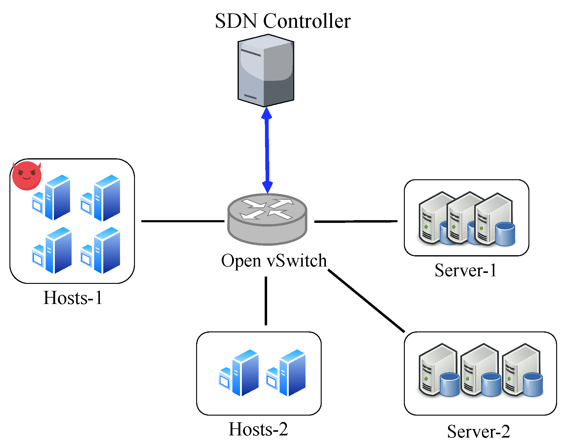
We implement flow table management schemes as applications running on the Ryu controller. For the data plane, we use Mininet with Open vSwitch 2.13.1 to build the network topology. The topology of the experimental network is depicted in
Figure 8. We use four attack hosts to generate flows to overflow the victim switch. The attackers use Scapy [
32] to generate probing packets and the attack traffic. We also deploy one host to replay the packets from traffic traces [
33] as benign background traffic. The flow table capacity is set to 1000.
To handle the packet-in messages, we deploy the
application on the controller, which provides the basic forwarding function. The match field is configured as <src_mac, dst_mac, src_ip, dst_ip>. For the random time mechanism, the controller assigns a value between 1 s and 15 s. For adaptive timeouts, we implement typical adaptive timeout algorithms, including Intelligent Timeout Master (ITM) [
15], SmartTime [
17], and TST [
19] (For TST, we only implement the adaptive timeout module with the initial timeout of 1 s.) according to the corresponding papers.
5.2. Evaluation of the Inferring Phase
We evaluate the performance of inferring different types of timeout strategy. As described in
Section 4, we obtain the initial timeout by probing the timeout values of new flow rules.
As depicted in
Figure 9, the timeout distribution varies widely among different timeout decision methods. For the fixed timeout setting, all flow rules have the same timeout value, which is consistent with the controller setting; for the random timeout strategies, the timeout value varies from 1 to 15; for the adaptive timeout setting, we observe that nearly all flow rules have a very small timeout value. These results prove that the attacker can probe timeouts with high accuracy, and thereby easily infer the type of timeout mechanism.
5.3. Evaluation of the Triggering Phase
In this experiment, we can evaluate the triggering phase to validate if the attacker can trigger flow rules with large timeouts under different timeout strategies.
For the adaptive timeout mechanism, we use the coarse-state-based method to trigger flow rules. We generate 100 attack flows and make them trigger flow rules with timeout values that are as large as possible. We record the returned timeout values (from the attacker hosts), which serve as the upper limit of the packet intervals in the maintaining phase, and compare them with the actual assigned timeout values (from the SDN controller). Ideally, the triggered flow rules should have timeout values close to the maximum value configured by the timeout assignment module. The results are shown in
Figure 10.
For TST, all attack flows can trigger flow rules with the idle timeout value of 3 s, the maximum timeout setting.The accuracy is 100%, so the results overlapped. For SmartTime and ITM, 98% of the flows can reach maximum timeouts, which is sufficient to launch the next attack phase. Considering that each flow requires up to four table-misses to trigger the maximum timeout, and only 2% of attack flows fail due to false probing responses, the results also demonstrate the high accuracy rate of the RTT-based measurement. These results demonstrate that our attack method can effectively trigger flow rules of specific states. However, if we recall the results presented in
Section 3, the typical attack methods in previous studies only triggered flow rules with small timeout values.
For the required minimal attack traffic rate, generating significantly larger timeout values proves beneficial in reducing the attack overhead. When flow rules are assigned with initial timeout values, each packet interval for the attack flows must not exceed the initial timeout threshold of 1 s. However, the attacker can induce the controller to deploy malicious flow rules with the maximum timeout value in the triggering phase, thus effectively reducing the minimum average attack rate (ranging from 1/3 for TST to 1/11 for ITM) compared to using the default timeout value in the aforementioned scenarios.
5.4. Evaluation of the Attack Effectiveness
We also implement the saturation attack program and evaluate its effectiveness as a whole process. We implement existing timeout decision algorithms and deploy monitoring programs on the SDN controller.
In the attack process, the generation rate of malicious flow rules is controlled. We use up to 80 flows to simultaneously generate malicious flow rules during the triggering phase. To comprehensively analysis of the attack’s impact on various network performance metrics, we demonstrate the attack’s effectiveness in three typical scenarios: (I) direct forwarding, (II) dropping request, and (III) rule eviction.
5.4.1. Impact on the Flow Table Utilization
We measure the flow table consumption of the victim switch with and without the attacks. In the attack scenario, we measure the number of flow rules generated by attack flows and benign background flows, respectively. As shown in
Figure 11, without the attack traffic, the number of flow rules ranges between 500 and 600, which is about half of the capacity. When the attack occurs in the attack scenario, as shown in
Figure 12, the number of flow rules can increase to 1000 at around 252 s. The result demonstrates that the saturation attack can effectively overflow the flow table.
We can observe that after the flow table is full, the number of rules fluctuates rather than staying at 100% all the time. The reason is that the background traffic fluctuates, and the controller cannot immediately insert new flow rules when the old ones expire. In our settings, the controller stops installing rules when it detects that the switch has no storage space. The flow table storage space can only be released after the installed rules in the switch expire due to a timeout. Then the controller detects the freed space by receiving the Flow-Removed messages, which is not a real-time process.
We also find that the number of flow rules for benign flows is less than that without the attack. After the flow table is saturated, the number of attack flows gradually increases while the number of benign flows decreases. The reason is that benign flows must compete with attack flows for the flow table space when the flow table is overflowed. However, the attack flow rules are persistently stored and occupy the storage space. Therefore, the controller cannot handle the benign requests.
5.4.2. Effectiveness against the Direct Forwarding Method
In this scenario, the controller forwards packets by packet-out messages instead of installing flow rules. We count the number of packet-in messages and measure how many packets are forwarded by the controller.
Figure 13 shows the number of packet-in requests with and without the attacks, respectively. Before the flow table is full, the numbers of packet-in messages are close in both scenarios. When the flow table is overflowed, the of packet-in rate increases significantly. After the flow table suffers saturation, the packet-in rate is 551 pps, while the average rate under the normal scenario is 350 pps.
We also measure the ratio of packet-in messages caused by background flows and attack flows after the table saturation. As shown in
Figure 14, 98% of the forwarded packet-ins are caused by benign traffic. The reason is that we limit the attack flow generation rate to prevent the rapid growth of malicious flow rules. Thus, defensive approaches against saturation attacks towards the controller cannot throttle the attack traffic, but may affect the benign traffic. Note that we allow up to 80 attack flows to trigger the rule installation simultaneously. The packet-in rates can be further reduced by configuring fewer attack flows.
To demonstrate the impact on the network performance, we measure the RTT of service requests sent to Server-1. We send 10 packets for each round of requests to calculate the RTT and repeat 10 rounds. The results are presented in
Figure 15. When no attack occurs, except for the first packet, which must be delivered by the controller, the average latency of subsequent packets is 1.16 ms. When the storage space is exhausted by attackers, the delay of all packets of new flows is about 7.2 ms, which is a significant increase.
5.4.3. Effectiveness against the Dropping Request Method
Then, we evaluate the impact in the scenario that the controller drops the packet-in request when the flow table is full. We measure the total number of packet-in requests and the dropped packet-in requests generated by benign and attack traffic, respectively.
The result is shown in
Figure 16. After the flow table occupation reaches 100%, more than 68% of the packet-in messages are dropped. This result demonstrates that the attack can cause high packet loss and degrade the network performance. Another observation is that more than 97% of the dropped packet-in messages come from benign traffic. This is because the packet-in rates of attack flows are lower than benign flows, so they are less likely to be dropped. This also indicates that from the defense perspective, it is hard to identify attack flows solely based on the packet-in messages.
To demonstrate the impact on the network performance from the data plane’s perspective, we measure the packet drop rate of benign service requests sent to Server-1. In each round, we measure the number of request retries before receiving a response. As shown in
Figure 17, 11 of the 15 rounds of requests cannot receive immediate responses. The flow requests require an average of four additional retries to be delivered properly. The reason is that when the flow table space is saturated, the SDN controller has to decline the packet-in messages. Flow requests can only pass through the switch if the corresponding flow rules are deployed.
5.4.4. Effectiveness against the Rule Eviction Method
Both of the previous methods lead to massive packet-in messages because the controller stops installing flow rules for flows, so the packets are still unmatched. Another countermeasure is the eviction strategy. In this method, the OpenFlow switch automatically deletes flow entries to make space for new ones. For the sake of generality, we use the eviction algorithm in the widely-used Open vSwitch. We evaluate whether benign background flows can replace the triggered attack flow rules.
Figure 18 shows the number of flow rules for malicious and benign flows. Since the replacement is performed on the switch side, the flow table utilization is almost always at 100% after the flow table is full. We can see that after overflowing the flow table, the injected malicious flow rules will not be replaced by benign flows. When the number of benign flow rules decreases, the attack flow immediately occupies the freed storage space and keeps the flow table full.
We also collect the information from the Flow-Removed messages to compare the number of evicted normal flow rules and malicious flow rules. The result is shown in
Figure 19. After the flow table is full, more than 82% of the deleted flow rules are benign flow rules. Note that when the flow table is full, the number of attack flow rules is approximately 50% of the flow table capacity. However, benign flow entries are more likely to be deleted when selecting flow entries. This indicates that the eviction strategy is more inclined to keep malicious flow rules rather than benign ones.
Upon further analysis of the results, we identify the cause of this. OvS implements the Least Recent Used (LRU) eviction method by selecting the entry that expires soonest for eviction. In our study, the controller assigns different timeouts for flows based on the packet inter-arrival time instead of using fixed timeout values. When assigned with different idle timeouts, flow rules with large timeouts are less likely to be evicted. During the attack process, we induce controllers to assign larger timeouts for attack flows. In the maintaining phase, we randomly select a value within the timeout range instead of resending the packet just before the flow rule expires. This approach makes it less likely for malicious flow rules to be deleted when selecting flow rules to evict, as they require a long time to expire. This experiment result also validates the effectiveness of triggering large timeouts in the triggering phase and using different packet intervals in the maintaining phase.
5.5. Effectiveness on the Load-Aware Strategy
We conduct another experiment to evaluate the attack performance where the controller adopts a feedback control to adjust the timeout setting. We use the classic feedback-control algorithm proposed in ITM [
15]. Due to the performance concern, we use fewer attack flows (20 simultaneous attack flows) to launch the attack. We compare (i) the flow table usage, (ii) the max timeout values, and (iii) the packet-in rates in both scenarios.
Figure 20 shows the flow table utilization. The flow table occupancy starts to reach its peak at around 443 s. Compared with the case without feedback control, benign flow entries occupies less space. Before the flow table is full, the number of benign flow entries is less than 400. The reason is that when the flow table occupation is beyond the
, the controller starts to reduce the timeout. With the smaller timeout, the number of benign flow rules is reduced. As shown in
Figure 21, the max timeout value is adjusted according to the flow table occupation. At 270 s, the max timeout is decreased to 1 s, the minimum timeout value. In
Figure 20, the number of benign flow flows declines sharply after 270 s.
We also evaluate the impact on the controller by measuring the number of packet-in messages. In
Figure 22, the packet-in rate is significantly higher after the flow table is completely overflowed at 443 s. By saturating the flow table space, the attack can cause an additional packet-in rate of approximately 140%. We also notice that the packet-in rate is higher than that in the normal traffic scenario, even before overflowing the flow table. Between the 270 s and 440 s (the flow table is not full), the average packet-in rate is about 8% higher than that of the normal scenario. The reason is that the controller begins assigning smaller timeouts due to high flow table occupancy before the overflow happens. Thus, benign flows with large packet intervals trigger more packet-ins.
Against the load-aware strategy, the attacker can only slightly degrade network performance by occupying flow table space and forcing the SDN controller to assign smaller timeouts. However, to cause severe performance degradation and disruption, the attacker must overflow the entire flow table.
5.6. Stealthiness
In this section, we evaluate the stealthiness of the proposed saturation attack considering existing anomaly detection mechanisms. Existing SDN defense mechanisms adopt different detection models but share similar detection metrics. Thus, we demonstrate the stealthiness by (1) the packet-in rates, (2) the controller overhead, and (3) the attack traffic rate, which are the key metrics that many recent defense methods [
29,
30,
31,
34,
35] use to detect network anomalies.
(1) Packet-In rates: We measure the number of packet-in messages sent to the controller with and without the attack. As shown in
Figure 23, before the flow table is full (around 250 s), there is no noticeable difference between the packet-in rates for the two scenarios. After the flow table is overflowed by malicious flows, the packet-in rate increases. Compared with the table-miss attack [
36], which targets saturating the control channel between the control and data planes, the flow table saturation attack incurs only a few additional packet-in messages. Even after overflowing the flow table, most packet-in requests are caused by benign flows. Therefore, existing defense mechanisms against the controller saturation attack cannot react to the flow table saturation attack.
(2) Controller overhead: Some detection mechanisms monitor the controller’s overhead [
37] to capture network anomalies. We measure the CPU usage of the Ryu controller with and without the attack. The results are shown in
Figure 24. Before the flow table is saturated, there is almost no difference between the two scenarios: the average CPU usage is 29.1% when there is no attack and is 29.3% in the attack scenario. Only after the flow table is overflowed at around 260 s, the CPU usage increases because of the additional packet-in requests. After the flow table is full, the average CPU load in the attack scenario is about 18% higher than the normal scenario.
(3) Attack traffic rate: We also measure the attack traffic rate to further demonstrate its stealth from the data plane’s perspective.
Figure 25a shows the attack traffic rates, and
Figure 25b shows the traffic rate of background traffic. As the attacker generates more flow rules in the flow table, the required attack traffic rate is higher. When overflowing the flow table, the rate of attack traffic is only tens of Kbps, which is significantly smaller than the benign background traffic.


