Article

A Novel Inverse Simulation Method of Helicopter Maneuvering Flight

1
Chinese Aeronautical Establishment, Beijing 100029, China
2
School of Aeronautic Science and Engineering, Beihang University, Beijing 100191, China
*
Author to whom correspondence should be addressed.
Appl. Sci. 2023, 13(12), 7214; https://doi.org/10.3390/app13127214
Submission received: 13 May 2023 / Revised: 7 June 2023 / Accepted: 13 June 2023 / Published: 16 June 2023
(This article belongs to the Section Aerospace Science and Engineering)

Abstract

:
In this article, a degeneration method of inverse simulation is proposed for a helicopter system flying pull-up and slalom maneuvers. This inverse simulation method has been successfully applied, and here, the results are compared with the flight test data and the reference data, which indicate that this method has fidelity and is effective. It is different from conventional inverse simulation methods (i.e., the differentiation method and the integration method), and can improve numerical stability during inverse simulation, because the core principle is to solve the output vector in each simulation time step, by degenerating the system of first-order differential equations into nonlinear equations.

1. Introduction

The conventional simulation solves the helicopter flight state response to selected control inputs, to generate a time history of the flight path. The inverse simulation conducts the reverse of that process, where the time history of a flight path is defined first, and the time histories of the flight states and control inputs are then solved using a series of numerical algorithms. It is an effective method for studying the maneuverability of aircraft [1]. This is because by using the inverse simulation to obtain the control inputs, we can check if the control inputs exceed the limits of the aircraft, and can also check if some key variables such as power, speed, angular velocity, etc., exceed the usage limits of the aircraft. If they exceed, it indicates that the aircraft cannot fly this maneuvering action, and needs to change the definition of the trajectory. If a certain limit is reached, it indicates that the aircraft’s ultimate maneuvering ability has been reached. The inverse simulation can also be used in the conceptual design of aircraft, to identify deficiencies in the design proposals during preliminary assessment [2]. Some other aspects of research, such as the flying quality evaluation [3], flying trajectory optimization [4], maneuvering strategies optimization [5], and flight dynamics characteristics [6], etc., can be conducted using the inverse simulation. This is a very helpful technique for aircraft design, and application in the aviation field.
The first inverse simulation was conducted in the 1930s, when a simple linearized aircraft model to study the effect of gusts was inverted [7]. Later, Etkin [8] discussed simple inverse simulation methods applied to problems such as achieving a prescribed response. Subsequently, an energy-based technique [9] that investigated the ability of helicopters to maneuver was proposed. However, the techniques required to achieve inverse simulation only came into early use in practical engineering in the mid-1980s, when a practical method of inverse simulation for studying helicopter agility was developed by Thomson and Bradley [10]. Their method was capable of simulating a wide range of maneuvers, and a wide range of practical problems [2,11].
To date, conventional inverse simulation methods can be mainly classified as differentiation methods, integration methods, and two time-scale methods [12]. The differentiation method discretizes a maneuver based on the numerical differentiation method, and solves the model at each time step using an iterative scheme. It has been adopted by many researchers [13,14,15], and has been updated and improved [16,17,18]. The integration method integrates the helicopter model through a time interval that is considerably greater than the integration time step while these control inputs are fixed [19,20,21]. It has been adopted to assess the reliability of simplified rotorcraft models in the evaluation of maneuvering potential [22]. Helicopters undergoing unsteady maneuvers can also be analyzed using this method [23]. The two time-scale methods attempt to reduce the helicopter system by considering that the translational equations of motion are solved, with the assumption that the rotational equations have attained a dynamic balance, with the angular velocity of zero [24,25].
This article presents a novel method of inverse simulation that names a degeneration method, by constructing a transitional vector, to prescribe the time histories of an output, and, meanwhile, to express the state vector of the dynamics system. Thus, the first-order differential equations can be degenerated into nonlinear equations in the process of inverse simulation. This degeneration method will be applied to a helicopter system. The new idea behind the method is that the quantitative relationships between the flight state and control input, as well as the prescribed output (i.e., the flight path), can be analyzed (or deduced) almost directly, without any complex numerical algorithm. Furthermore, the method has good versatility and robustness, and has no integration process, compared with integration methods. It does not need to adopt the two time-scale methods, and only needs to use the differentiation method to discretize the Euler angle derivatives.
The article has the following structure. The degeneration method is proposed in Section 2. Section 3 develops the theoretical application of the degeneration method to the helicopter system. Section 4 compares the numerical results and the flight test, by using a case study of a helicopter flying a dynamic pull-up maneuver, and conducts a case study of a helicopter flying a slalom-course maneuver. Our discussion and conclusions are given in Section 5.

2. Degeneration Method

The conventional simulation can be written as a system of first-order differential equations:
x ˙ = f ( x ,   u )
where x and u are the state and control vectors, respectively. To conduct an inverse simulation, an output vector y , which is a function of the state vector x , needs to be prescribed in the course of the simulation:
y DES = g ( x )
Thus, the inverse simulation finds the control time histories u ( t ) under the action of Equation (1) to generate a prescribed output vector y DES . To make progress, Equation (2) is usually differentiated to obtain:
y ˙ DES = g x ( x ) x ˙
Substituting Equation (1) into Equation (3) gives:
y ˙ DES = g x ( x ) f ( x ,   u )
Some numerical algorithms are adopted to solve this equation, such as the differentiation method and the integration method. However, the functional matrix g x ( · ) needs to be evaluated when using these methods. This inevitably suffers some numerical errors (e.g., low-amplitude, high-frequency oscillations superimposed on the low-frequency waveform) and makes the results dependent on the simulation time step to some extent. These numerical instabilities have been studied thoroughly by Lin and Lu [26], Thomson and his colleagues [12,20], and others.
In the process of inverse simulation, to avoid evaluation of this g x ( · ) and to achieve better versatility and robustness, a novel method called the degeneration method is developed here. The basic principles of our method consist of the following two main aspects: degeneration based on a transitional vector, and determination of the transitional vector.

2.1. Degeneration Based on a Transitional Vector

We assume that a prescribed time history exists of a transitional vector η ( t ) that can directly express y ˙ DES in the form:
y ˙ DES = g * ( η ( 0 ) ( t ) ,   η ( 1 ) ( t ) , ,   η ( n ) ( t ) )
Meanwhile, each element x i in the state vector x can be expressed in the form:
x i ( r ) = h r ,   i ( η ( 0 ) ( t ) ,   η ( 1 ) ( t ) , ,   η ( n ) ( t ) )
where i denotes the ith element in the state vector x , r is the time derivative order of x i , which equals 0 or 1, and n is the time derivative order of η ( t ) .
Substituting Equation (6) into Equation (1) gives:
h 1 ( η ( 0 ) ( t ) ,   η ( 1 ) ( t ) , ,   η ( n ) ( t ) ) f ( h 0 ( η ( 0 ) ( t ) ,   η ( 1 ) ( t ) , ,   η ( n ) ( t ) ) ,   u ) = 0 N × 1
where h r ( · ) = [ h r ,   1 ( · ) ,   h r ,   2 ( · ) ,   ,   h r ,   N ( · ) ] T , and N is the dimension of h r ( · ) . Thus, the first-order differential equation, i.e., Equation (1), can be degenerated into these nonlinear equations. The time history of the control vector, u , can be attained by solving Equation (7) in each simulation time step. It makes sense, and improves the numerical stability, because the nonlinear equations can be easily solved, for example, using the Levenberg–Marquardt algorithm for nonlinear least-squares minimization [27], without evaluation of g x ( · ) .

2.2. Determination of the Transitional Vector

If this time history η ( t ) is realistic, a basic polynomial scheme that can be used to express any element in the vector η ( t ) , then:
χ ( t ) = i = 0 M a i · t i
where χ ( t ) denotes the element in the vector η ( t ) . To obtain the time histories χ ( t ) , the coefficient a i and the highest power of the polynomial M need to be attained first.
Some of the boundary conditions should be prescribed, to determine a i and M . In general, χ ( t ) , χ ˙ ( t ) , and χ ¨ ( t ) of the two adjacent simulation time points, e.g., t 1 = 0 sec and t 2 = 1.0 sec, can be taken as the boundary conditions to obtain three necessary boundary conditions of the start state:
{ χ * ( t 1 ) = i = 0 M a i · t 1 i χ ˙ * ( t 1 ) = i = 1 M a i · i · t 1 i 1 χ ¨ * ( t 1 ) = i = 2 M a i · i · ( i 1 ) · t 1 i 2
and three optional boundary conditions of the end state:
{ χ * ( t 2 ) = i = 0 M a i · t 2 i χ ˙ * ( t 2 ) = i = 1 M a i · i · t 2 i 1 χ ¨ * ( t 2 ) = i = 2 M a i · i · ( i 1 ) · t 2 i 2
where the superscript * denotes an exact known quantitative value. A system of algebraic equations, made up of the above necessary and optional boundary conditions, can be solved to attain a i on the premise of a known value of M . Note that all the boundary conditions of the start state need to be prescribed to obtain an exact start state, and not all the boundary conditions of the end state need to be prescribed, because the end state can be attained by this polynomial scheme, at least based on the boundary conditions of the start state (in this case, M = 2 ) in the simulation. Thus, the boundary condition, i.e., Equation (9), is necessary; the boundary condition, i.e., Equation (10), is optional; and the value of M can be selected as between 2 and 5, to match the number of boundary conditions (from 3 to 6), and enclose the system of algebraic equations.
Generally, because there are more than two time points that are used to prescribe the boundary conditions of χ ( t ) , we choose the two adjacent time points as a calculation stage. In other words, n time points (the value of n must be greater than 2) have ( n 1 ) calculation stages.

3. Application to the Helicopter System

According to the right-hand rule of the frame system, an earth-fixed inertial frame ( o E x E y E z E ) is defined at an arbitrary reference point ( o E ) on the ground, with the axes o E x E , o E y E , and o E z E toward the respective east, north, and vertical up. Following this, a flight-path frame ( o x P y P z P ) and a body frame ( o x B y B z B ) are then defined at the helicopter center of gravity ( o ), with the axis o x P toward the direction of flight velocity vector V P , and the axis o x B toward the helicopter nose, and parallel to the cabin floor. Figure 1 shows these definitions of the frame system, where Φ BP = [ ϕ BP ,   θ BP , ψ BP ] T is the Euler angle between frames o x B y B z B and o x P y P z P . ψ BP also indicates the sideslip angle of the helicopter, and ψ PE and θ PE are the yaw angle and climbing angle of the flight path relative to frame o E x E y E z E , respectively, which can be written as a vector form of Φ PE = [ 0 ,   θ PE , ψ PE ] T for convenience.
The motion of a helicopter in the air can, in general, be described by a combination of rotations and translations. The rotations include pitch around axis o y B , roll around axis o x B , and yaw around axis o z B . The translations include move forward or backward along axis o x B , move right or left along axis o y B , and move downward or upward along axis o z B . If the helicopter is regarded as a rigid body, a conventional helicopter flight dynamics system can be written in the form:
{ m B V ˙ B + ω B × ( m B V B ) = F B AERO + m B · g B I B ω ˙ B + ω B × ( I B ω B ) = M B AERO T E u l e r · Φ ˙ B = ω B                                                                                              
where V B = [ u B ,   v B , w B ] T 3 is the body translational velocity, ω B = [ p B ,   q B , r B ] T 3 is the body angular velocity, Φ B = [ ϕ B ,   θ B , ψ B ] T 3 contains the respective body roll, pitch, and yaw angles, m B 1 is the mass, I B 3 × 3 is the inertia matrix, g B 3 is the acceleration of gravity in the frame o x B y B z B , T E u l e r 3 × 3 is the Euler transformation matrix, and F B AERO 3 and M B AERO 3 are the respective resultant aerodynamic force and resultant aerodynamic moment generated by the main rotor, tail rotor, fuselage, and horizontal and vertical tails for a single-rotor helicopter.
Three processes (i.e., the construction of a transitional vector, the development of the functional forms of the state vector, and the degeneration of the first-order differential equations) need to be carried out when using the degeneration method to conduct inverse simulation.

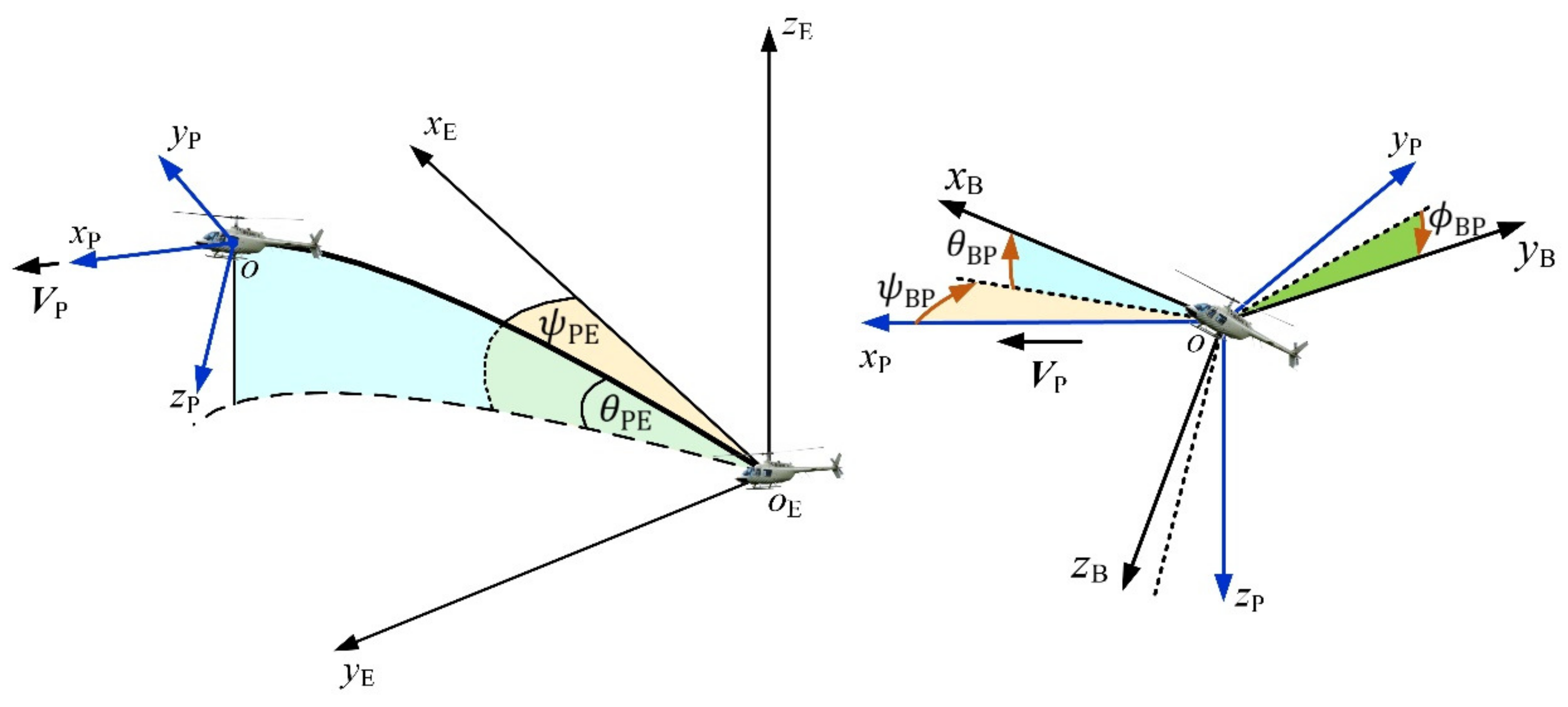
3.1. Construction of a Transitional Vector

In the inverse simulation of the helicopter system, the prescribed output vector y DES usually contains the elements x E ,   y E ,   z E and ψ BP [15]. Thus, its first-order differential form is:
y ˙ DES = [ x ˙ E y ˙ E z ˙ E ψ ˙ BP ] = ( T z ( ψ PE ) T y ( θ PE ) 0 3 × 1 0 1 × 3 1 ) [ S ˙ P ψ ˙ BP ]
where T y ( · ) and T z ( · ) are the Euler transformation matrices relative to the respective y- and z-axes. S ˙ P = [ S ˙ P ,   0 ,   0 ] T 3 , S P is a displacement variable, and S ˙ P is the scalar of the flight velocity, i.e., V P .
Thus, the prescribed vector η ( t ) can be constructed in the form:
η ( t ) = [ S P ,   θ PE , ψ PE ,   ψ BP ] T   or   η ( t ) = [ V P ,   θ PE , ψ PE ,   ψ ˙ BP ] T
Because V P and θ PE are in the longitudinal channel, and ψ PE and ψ BP are in the directional channel, the constructed vector η ( t ) can theoretically prescribe almost any three-dimensional maneuvering flight. Thus, our method has good versatility. Note that although the element ψ BP does not affect the elements of the flight path, i.e., x ˙ E , y ˙ E , and z ˙ E , different descriptions of ψ BP can indicate different maneuvers, as follows:
  • ψ ˙ BP = 0 and ψ BP = 0 indicate a maneuver with no sideslip; e.g., pull-up and hurdle-hop.
  • ψ ˙ BP = 0 and ψ BP 0 indicate a maneuver with a certain sideslip; e.g., sidestep and sideslip.
  • ψ ˙ BP 0 indicates a maneuver with a certain yawing rate; e.g., hovering turn and pirouette.

3.2. Development of the Functional Forms of the State Vector

Here, we use the prescribed time histories η ( t ) to develop the functional forms of the state vector x . The state vector x of the helicopter system includes the elements V B , ω B , and Φ B :
x = [ V B ,   ω B ,   Φ B ] T
Through coordinate system transformation, V B is deduced in the form:
V B ( r ) = T x ( ϕ BP ) T y ( θ BP ) T z ( ψ BP ) V P ( r )
According to the angular velocity composition theorem of rigid body motion [28], ω B can be deduced in the form:
ω B ( r ) = T x ( ϕ BP ) T y ( θ BP ) T z ( ψ BP ) [ e x ,   e y ,   T y ( θ PE ) T x ( 180 ° ) e z ] Φ PE ( r + 1 )                                     + [ e x ,   T x ( ϕ BP ) e y ,   T x ( ϕ BP ) T y ( θ BP ) e z ] Φ BP ( r + 1 )
where e x , e y , and e z are the unit vectors along the respective x-, y-, and z-axes, and T x ( · ) is the Euler transformation matrices relative to the x-axis.
The spatial position of the axes o x B and o y B in frame o E x E y E z E can indicate the quantitative value of the elements of Φ B
θ B = arcsin ( e x , E z )
ϕ B = {                                   0                               ,       e y , E Z = 0   arccos ( e 1 · e y , E | e 1 | )   ,       e y , E Z > 0       arccos ( e 1 · e y , E | e 1 | )   ,       e y , E Z < 0
ψ B = atan ( e x , E Y e x , E X )
where:
e i , E = [ e i , E X e i , E Y e i , E Z ] = T x ( 180 ° ) T z ( ψ PE ) T y ( θ PE ) T z ( ψ BP ) T y ( θ BP ) T x ( ϕ BP ) e i ,   B
where the subscript i denotes x or y , e i ,   B denotes the unit vectors e x or e y in frame o x B y B z B , e i , E denotes the unit vectors e x or e y in frame o E x E y E z E , and e 1 = [ e x ,   E Y , e x ,   E X ,   0 ] T 3 .

3.3. Degeneration of the First-Order Differential Equations

To degenerate the first-order differential equations, functional forms of some other variables, i.e., F B AERO and M B AERO , as well as g B in Equation (11), need to be developed.
Generally, collective ( δ C ), longitudinal cyclic ( δ B ), lateral cyclic ( δ S ), and pedal ( δ R ) controls are used to manipulate F B AERO and M B AERO , to fly the helicopter. In detail, collective, longitudinal cyclic, and lateral cyclic controls are used to control the main rotor, and pedal control is used to control the tail rotor. Note that F B AERO and M B AERO are also dependent on the state vector of the helicopter system. Thus, these can be deduced in the forms:
{ F B AERO = f F ( V B , ω B ,   Φ B ,   U 4 × 1   )   M B AERO = f M ( V B , ω B ,   Φ B ,   U 4 × 1   )  
where the control vector U 4 × 1 = [ δ C , δ B , δ S , δ R ] T 4 .
g B can be written in the form:
g B = T x ( ϕ BP ) T y ( θ BP ) T z ( ψ BP ) T y ( θ PE ) [ 0 0 g ]
where g 1 is the acceleration of gravity.
By combining with the prescribed vector η ( t ) , the functional forms of the state vector x , and Equations (21) and (22), the degenerated functional form of Equation (11) can be written in the form:
6 × 6 ( V P , V ˙ P ,   Φ PE ,   Φ ˙ PE ,   Φ ¨ PE ,   Φ BP ,   Φ ˙ BP ,   Φ ¨ BP ,   U 4 × 1 ) = 0 6 × 1
The time derivatives of ϕ BP and θ BP are developed based on the one differentiation-based approach [29]:
{ ( ϕ BP ( r + 1 ) ) m = ( ϕ BP ( r ) ) m ( ϕ BP ( r ) ) m 1 Δ t   ( θ BP ( r + 1 ) ) m = ( θ BP ( r ) ) m ( θ BP ( r ) ) m 1 Δ t  
where m represents the mth simulation iteration.
Thus, Equation (23) can be further written in the form:
6 × 6 [   η m ( n ) ( t ) ,   ( ϕ BP ) m 2 ,   ( θ BP ) m 3 , ( ϕ BP ) m 1 ,   ( θ BP ) m 1 ,   ( ϕ BP ) m ,   ( θ BP ) m , ( U 4 × 1 ) m ] = 0 6 × 1
where n equals to 0, 1 or 2. Because η m ( n ) ( t ) is known due to the prescribed flight path, there are six unknown variables, i.e., ( ϕ BP ) m , ( θ BP ) m , and ( U 4 × 1 ) m in the mth iteration. Thus, this nonlinear equation can be enclosed in each iteration, and degeneration can be realized.

4. Case Studies and Results

To validate the degeneration method, and illustrate its versatility and robustness, the following case studies on longitudinal and lateral/directional maneuvers are presented.

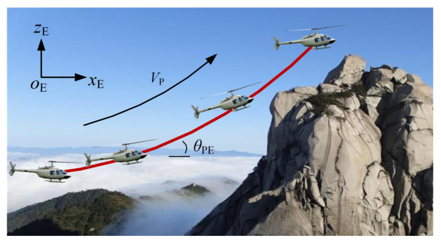
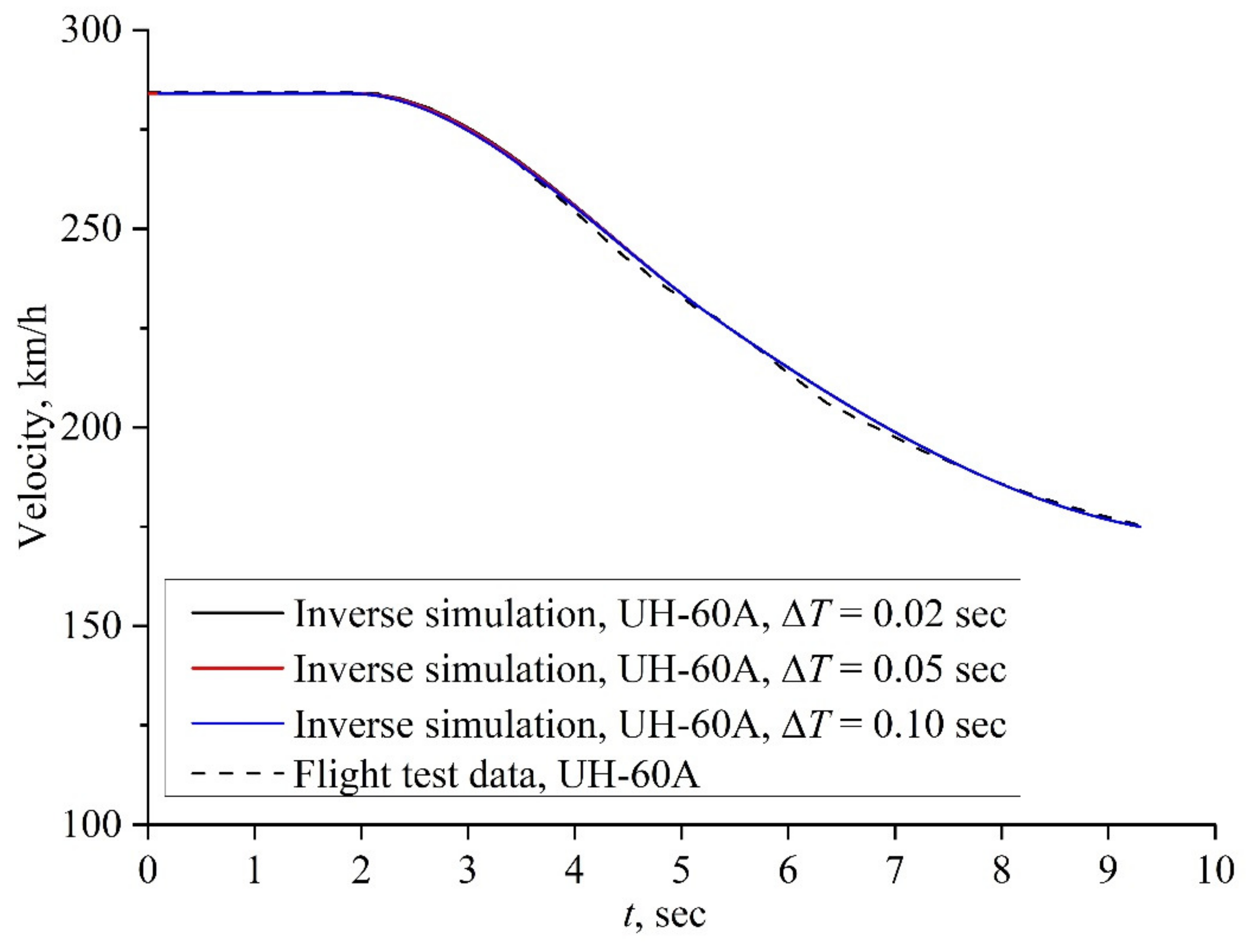
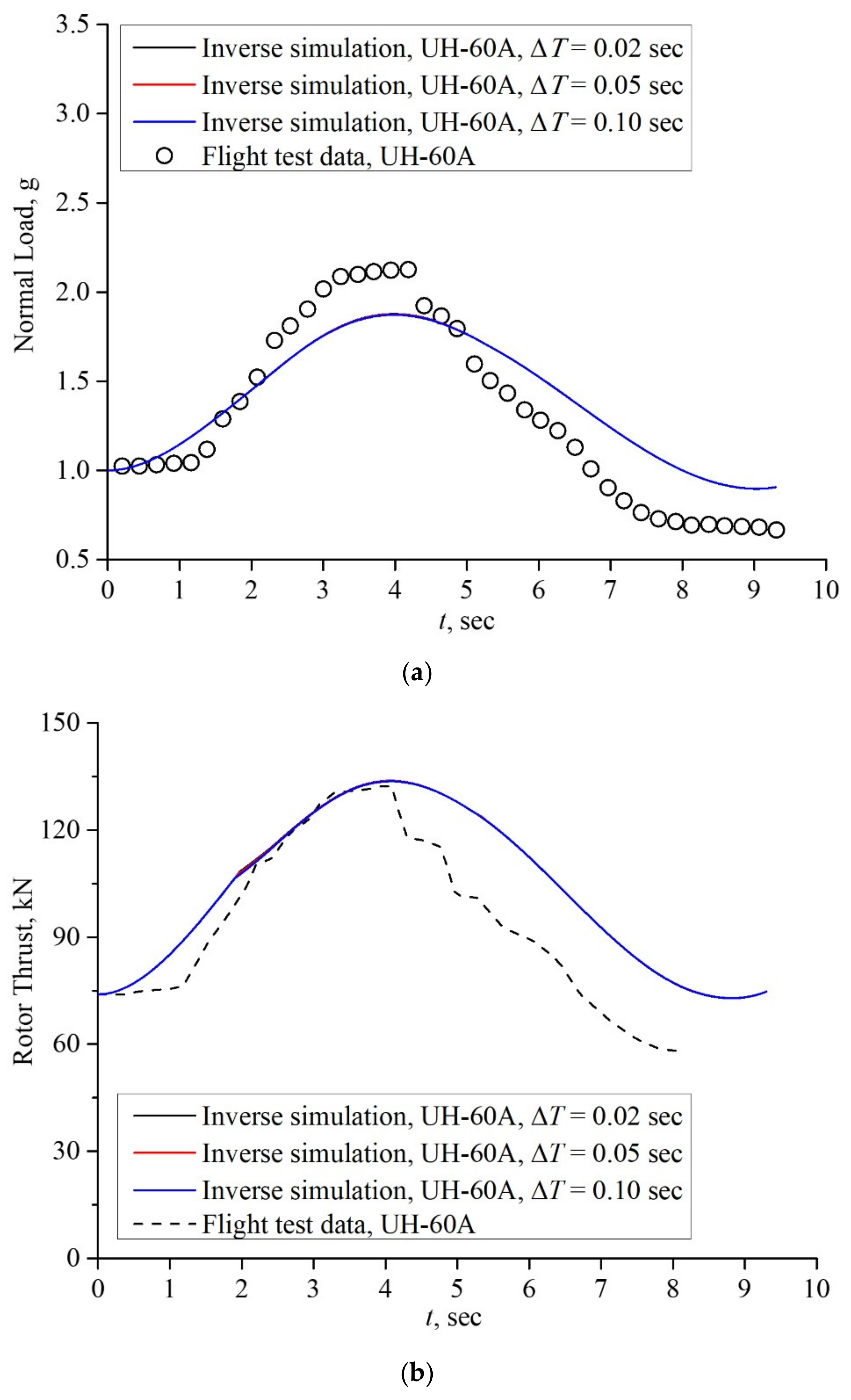
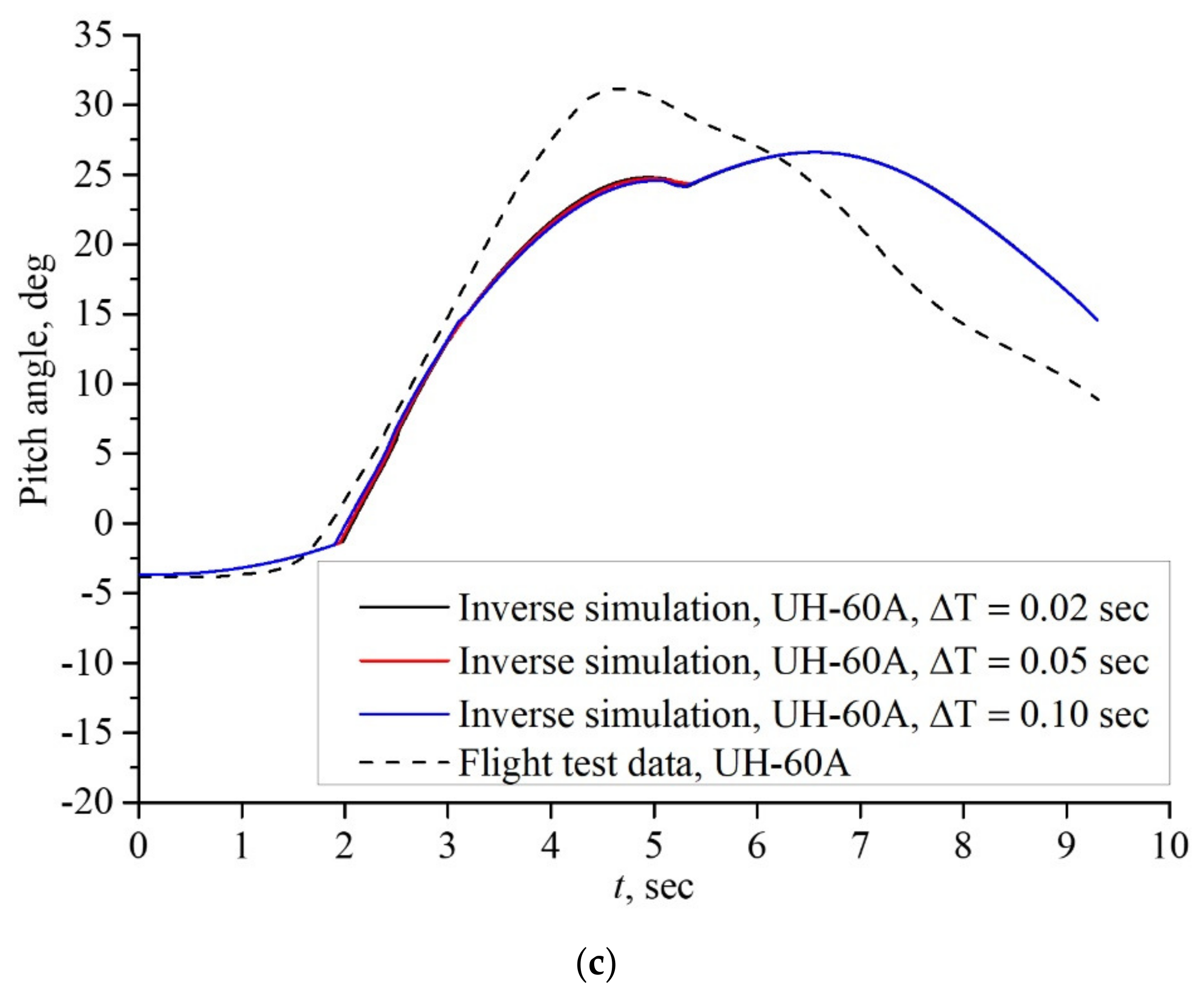
4.1. Case I: Pull-Up Maneuver

To validate our novel inverse simulation method, a case study of a helicopter flying a dynamic pull-up maneuver (in the longitudinal/vertical channel) was conducted. This maneuver was based on the Utility Tactical Transport Aerial System (UTTAS) maneuver of the original UH−60A design specification [30]. It was an instantaneous down-to-up turning maneuver in the vertical plane, and was designated by the Counter 11029 flight from the UH−60A flight test database, which is a terrain-avoidance maneuver in the longitudinal/vertical channel, and is initiated from a high-speed steady flight by pitching-up the helicopter for a rapid gain in altitude [31]. A sketch of the pull-up maneuver is shown in Figure 2. The maneuver lasted for approximately 9.3 s, reaching a maximum load factor of 2.12 g.
The relevant parameters of the UH−60A helicopter for the inverse simulation are shown in Table 1. By using rotor vortex, blade element, and rotor momentum theories [32], the conventional flight dynamics of the UH−60A helicopter can be developed (see [33,34,35]). In this model, the fuselage, horizontal, and vertical tail aerodynamics modeling is mainly based on wind tunnel data from NASA [36]. Tail rotor aerodynamics modeling is based on rotor momentum theory. The main rotor aerodynamics modeling is based on rotor vortex and element theories.
The pull-up maneuver only involves the elements in the longitudinal channel; i.e., V P and θ PE in the transitional vector η ( t ) . Thus, these directional elements ψ PE and ψ ˙ BP can be set as zero in the whole time histories. The boundary conditions of the time histories V P and θ PE are shown in Table 2. In detail, four time points of V P and two time points of θ PE are used to prescribe, according to the nature of this pull-up maneuver. Here, because the transitional element V P is a rate variable, the displacement variable S P is also used to follow the definition of the polynomial scheme, i.e., Equation (8). The boundary value of S P of time point 1 (i.e., the start) can be set as zero, and its values at the other time points are not necessary, because they can be inherited from the previous calculation stage.
To illustrate the numerical stability of the degenerated method, three simulation time steps (i.e., Δ T = 0.02 s, Δ T = 0.05 s, and Δ T = 0.10 s) are adopted. The primary results are shown in Figure 3, Figure 4, Figure 5 and Figure 6, and indicate that our method has good numerical stability and robustness, because the results are independent of these simulation time steps. The inverse simulation results regarding the maneuvering flight height and velocity are shown in Figure 3 and Figure 4. Corresponding flight test data are also shown in these figures. It can be concluded that the inverse simulation results are in good agreement with the flight test data. Thus, the prescribed boundary conditions outlined in Table 2 can describe well the flight path of the pull-up maneuver.
The normal load factor, pitch angle, and rotor thrust in the longitudinal channel are compared with the flight test data. Because the effects of the unsteady aerodynamics and the dynamic stall of the main rotor in the helicopter flight dynamics model have not been considered in this case study, the present peak normal load factor in Figure 5a only reaches 1.88 g (slightly lower than the flight data of 2.12 g), although the peak trimming rotor thrust in Figure 5b matches the flight data. The present peak pitch angle in Figure 5c is lower than the flight data, but these show a similar overall trend. In general, our inverse simulation results are credible, indicating that the degeneration method is reasonable and effective.
Figure 6 shows the time histories of the cockpit controls and the stabilator angle during the UTTAS pull-up maneuver. To realize a pull-up maneuver, two primary controls (i.e., longitudinal cyclic and collective sticks) are required. In detail, the longitudinal cyclic control stick is moved backward, and the collective control stick is put down, to enter the maneuver. Then, the longitudinal cyclic control stick is moved forward, and the collective control stick is raised, to recover from the maneuver.
In addition, the stabilator of the helicopter (i.e., the flexible horizontal tail) is controlled automatically by the flight control system, and depends on the flight velocity; and the collective controls the stabilator angle changes, from 1.0 deg to approximately 7.0 deg, during the whole pull-up maneuver, to provide an additional pitch moment for the helicopter. Note that the increase in the stabilator angle generates a pitching-down moment, while the decrease in the stabilator angle generates a pitching-up moment. Thus, the evident phenomenon is that the minimum value reaches approximately −1.0 deg when entering the maneuver (in this case, the helicopter needs a pitching-up moment, to quickly increase the pitch attitude), and the angle needs to be gradually increased when recovering from the maneuver (in this case, the helicopter needs a pitching-down moment, to restrain the increasing trend of the pitch attitude). Our method and the inverse simulation results illustrate this phenomenon well.

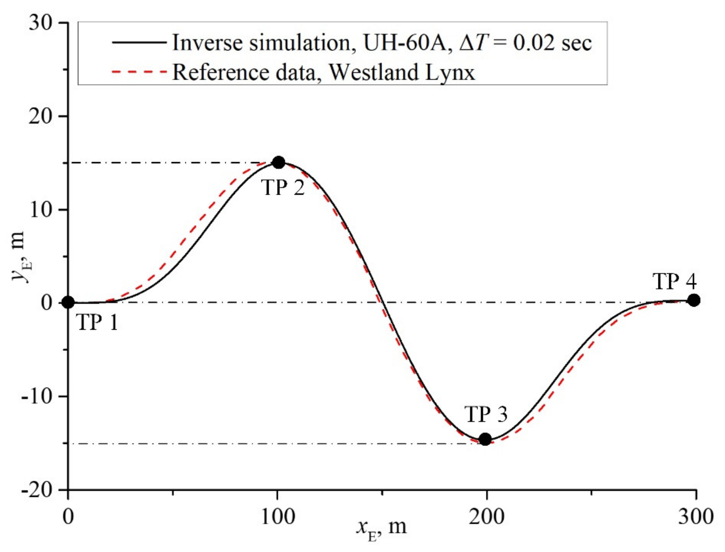
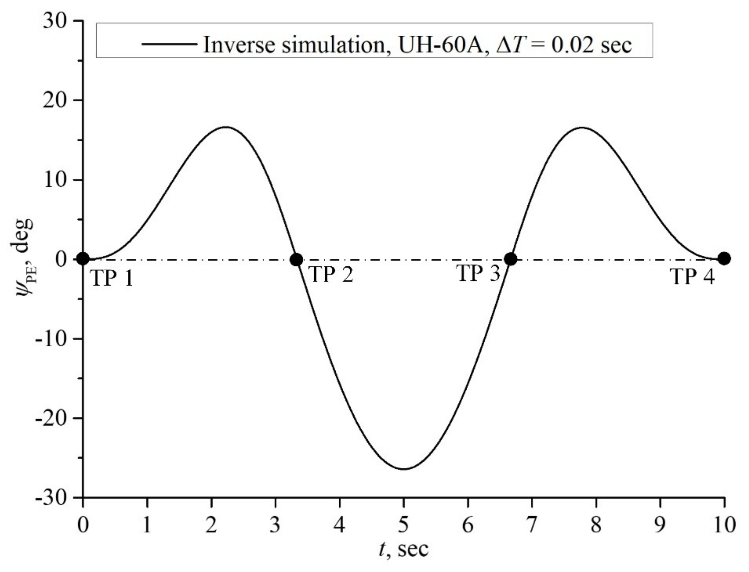
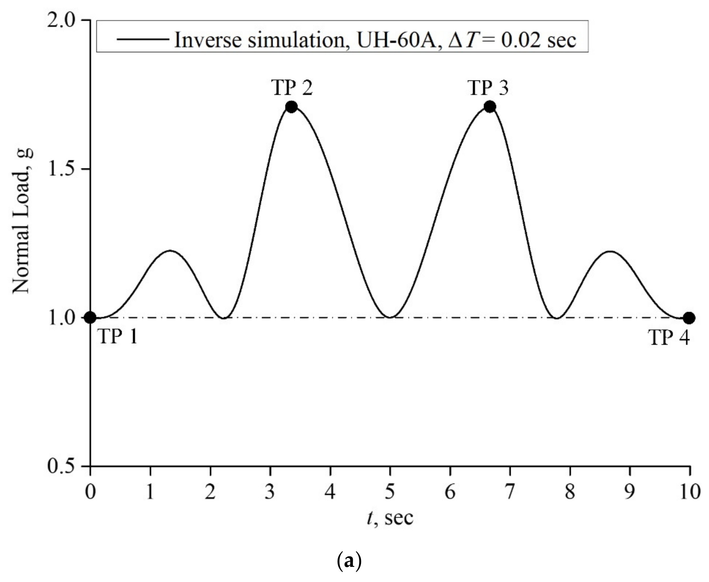
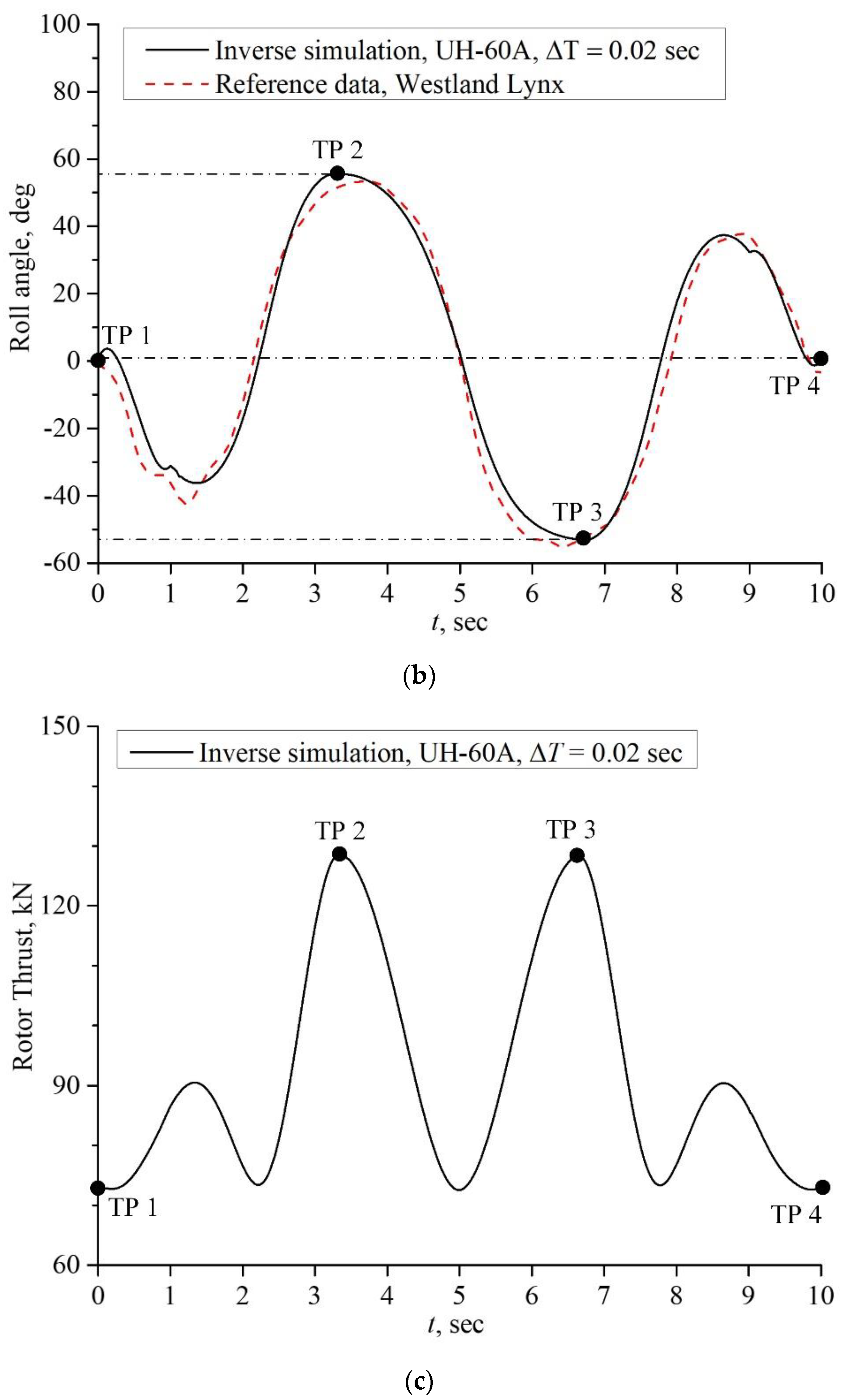
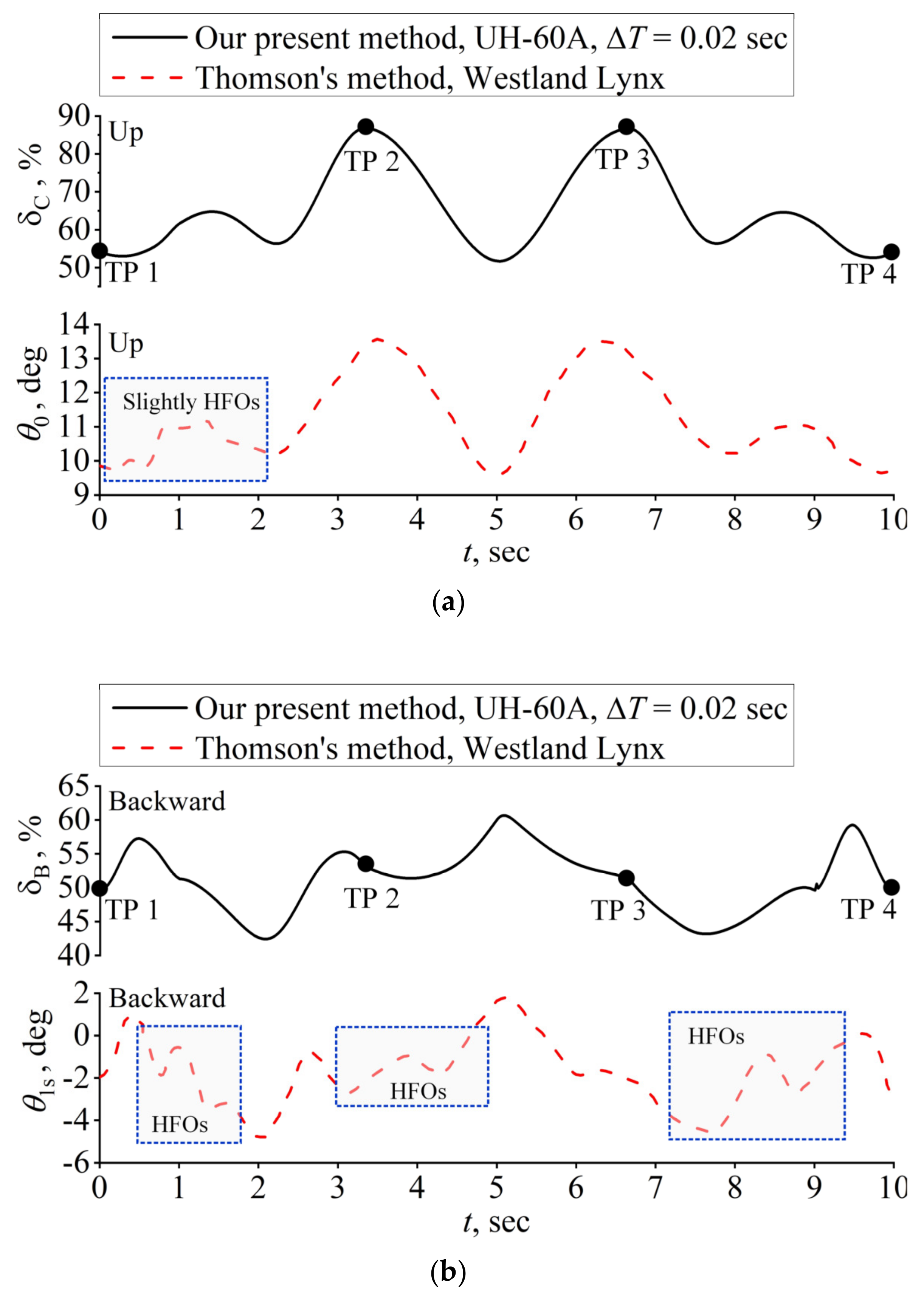
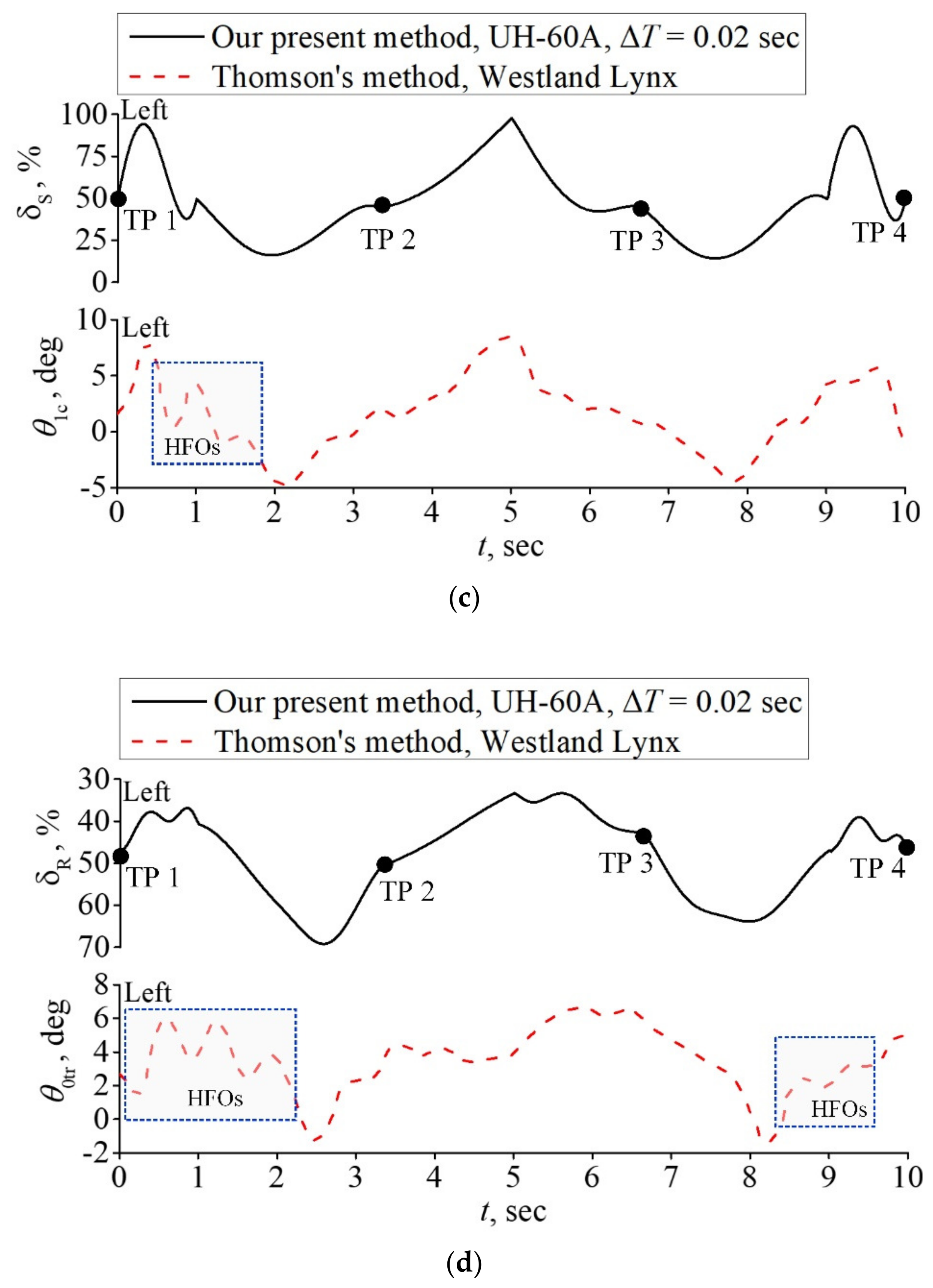
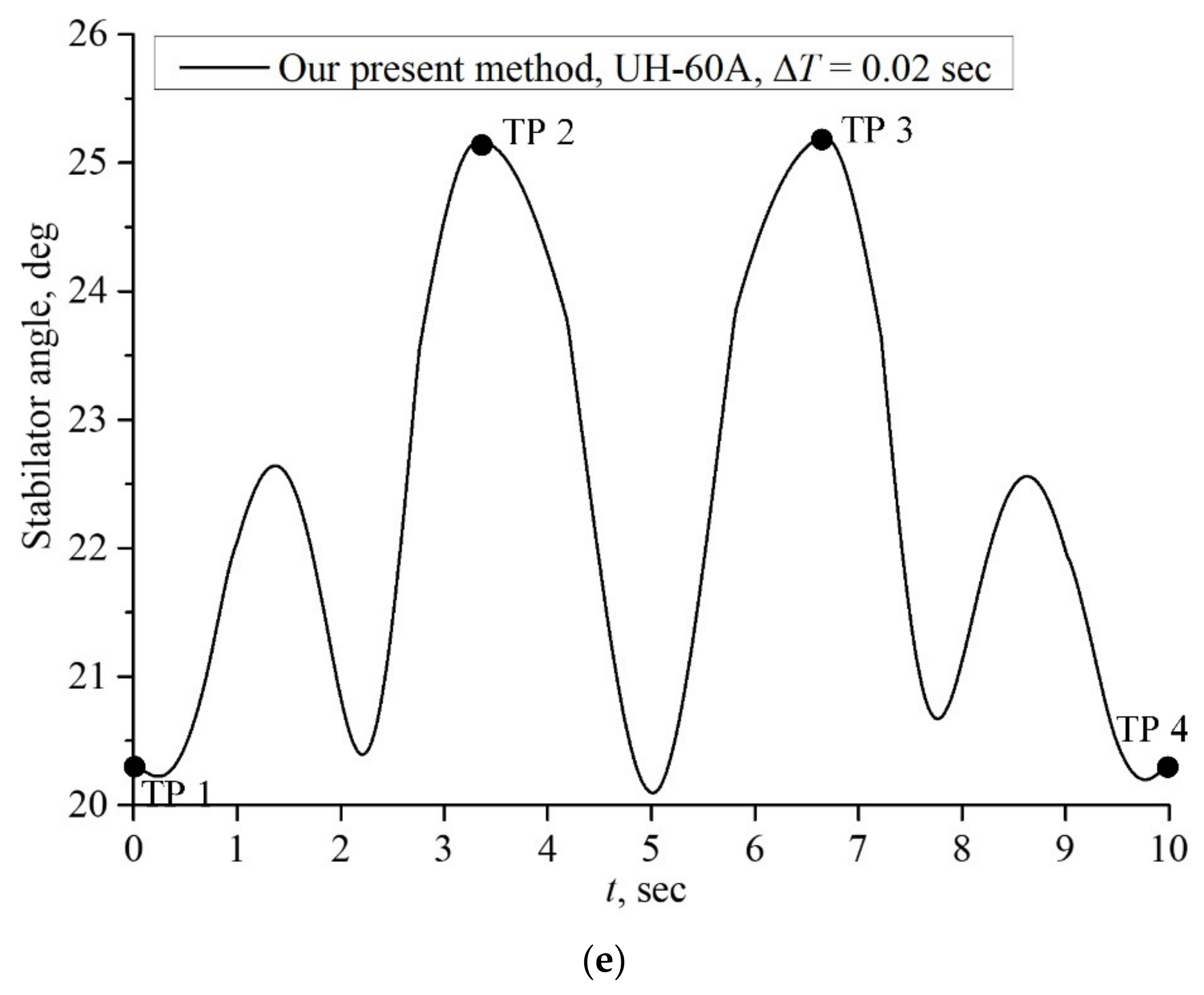
4.2. Case II: Slalom Maneuver

The slalom maneuver is described in the ADS-33 requirements document [37]. It is an instantaneous right-to-left or left-to-right turning maneuver in the horizontal plane. It also initiates level, unaccelerated flight, and lines up with the centerline, and is followed by a smooth turn to the left, followed by one to the right. According to the ADS33 requirements, the turns will be at least 50 ft (15.24 m), with a maximum lateral error of 50 ft (15.24 m), and the flight velocity through the maneuver must not be less than 40 knots or 60 knots (74.08 km/h or 111.12 km/h), respectively. In this case study, an idealized slalom maneuver proposed by Thomson [7] was conducted, to illustrate the degeneration method, but we used the UH−60A helicopter, instead of the Westland Lynx helicopter mentioned in Thomson’s article. The maneuver lasted for 10 s, the total distance was 300 m ( s = 100   m , Figure 7), the lateral displacement, h , was 15 m, and the flight velocity, V P , was 60 knots (111.12 km/h).
The slalom maneuver only involves the elements ψ PE and V P in the transitional vector η ( t ) . The remaining elements θ PE and ψ ˙ BP can be set to zero. Because the flight velocity, V P , is a constant in the whole process of this maneuver, it is not necessary to prescribe its boundary conditions. The boundary conditions of the yaw angle, ψ PE , are shown in Table 3. In detail, four time points are needed according to the nature of this idealized slalom maneuver. Time points 1 and 4 are the respective start and end, and time points 2 and 3 indicate the specific locations of the negative and positive maximum angular rates, respectively. The values of these maximum angular rates must match the maximum lateral displacement.
The primary results of the inverse simulation are shown in Figure 8, Figure 9, Figure 10 and Figure 11, and the simulation time step is selected as 0.02 s. Because, at present, there is a lack of flight test data and reference data of the UH−60A flying this idealized slalom maneuver, some of our results were compared with the inverse simulation results concerning the Westland Lynx helicopter flying the idealized slalom maneuver in Thomson’s literature [7]. Figure 8 shows the flight path, which indicates that the results are in good agreement with each other, although they involve different helicopter systems. The results of the prescribed variable, ψ PE , are shown in Figure 9. In the process of the slalom maneuvering flight, the maximum lateral displacement reached 15 m, which met the requirement of this idealized slalom maneuver. The positive maximum yaw angle was above 15 deg, and the negative maximum yaw angle was below −25 deg.
The time histories of the normal load factor, roll angle, and rotor thrust are shown in Figure 10. In particular, the roll angle is compared with Thomson’s inverse simulation results. These also match well with each other. In the process of the slalom maneuvering flight, the maximum normal load reached approximately 1.7 g, and the maximum rotor thrust reached approximately 130 kN.
Figure 11 shows the time histories of the cockpit controls and the stabilator angle during the slalom maneuver. The controls (i.e., collective pitch θ 0 , longitudinal cyclic pitch θ 1 s , lateral cyclic pitch θ 1 c , and tail rotor collective pitch θ 0 tr ) of Thomson’s inverse simulation results are also shown in Figure 11, to discuss the fidelity of our inverse simulation results. The changing trends of the controls are consistent with each other, although the helicopter system was different. More importantly, because our results for the time histories of the cockpit controls, which can be seen clearly in Figure 11a–d, have no high-frequency oscillations (HFOs), our method seems to be more robust than Thomson’s method [7]. It can also be noted that to realize a slalom maneuver, primary control (i.e., the lateral cyclic stick) is required. In particular, the helicopter initially rolled to the left (negative roll angle, see Figure 10b), due to an initial pulse of the lateral cyclic equivalent to a nearly full deflection of the stick. This phenomenon is consistent with Thomson’s results. In addition, the stabilator angle changed from approximately 20 deg to approximately 25 deg during the whole slalom maneuver, to provide an additional pitch moment for the helicopter. However, the changing range is smaller than that in the pull-up maneuver (i.e., Case I), due to the constant value of the flight velocity.

5. Discussion and Conclusions

A degeneration method of inverse simulation is proposed in this article, and was successfully applied to a helicopter system flying pull-up and slalom maneuvers. The inverse simulation results are compared with the flight test data and the reference data, which indicate that this method has fidelity and is effective. It is different from the conventional inverse simulation method, and can improve the numerical stability during inverse simulation, because the core principle is to solve the output vector in each simulation time step, by degenerating the system of first-order differential equations into nonlinear equations.
One advantage of the method is that it can invert the helicopter model, and simulate almost any maneuver in the longitudinal, lateral, and directional channels, and even any maneuver in the three-dimensional space, by introducing a transitional vector that can express the output and state vectors at the same time. Thus, our method has good versatility. In addition, because the present results are independent of simulation time steps, and the results of the time histories of the cockpit controls have no high-frequency oscillations (HFOs), our method also demonstrates good robustness. However, there are still two derivatives of Euler angles that cannot be directly expressed in explicit forms; thus, these angles have to be expressed numerically, using a differentiation-based approach.
We applied our novel inverse simulation method to the helicopter system in the maneuvering flight, and successfully obtained the required control inputs. These inverse simulation ideas can also be further applied by those working on inverse dynamics problems, in areas such as fixed-wing aircraft, unmanned aerial vehicles, rockets, and even robotics, and in other industrial fields, such as the direct trajectory control of ground vehicles and surface vessels, and even trajectory optimization problems in spacecraft. Next, we will further develop and improve this method, and attempt to conduct in-depth research on the direct trajectory control of any aircraft, any ground vehicle, and even any surface vessel, using this method.

Author Contributions

Conceptualization, G.L. and Y.C.; Methodology, G.L. and Y.C.; Software, G.L.; Validation, G.L. and Y.C.; Formal analysis, Y.C.; Writing—original draft, G.L.; Writing—review & editing, Y.C. All authors have read and agreed to the published version of the manuscript.

Funding

This research received no external funding.

Institutional Review Board Statement

Not applicable.

Informed Consent Statement

Not applicable.

Data Availability Statement

Enquiries about data availability should be directed to the authors.

Conflicts of Interest

The authors declare that they have no conflicts of interest.

References

  1. Anderson, D. Modification of a generalized inverse simulation technique for rotorcraft flight. Proc. Inst. Mech. Eng. Part G J. Aerosp. Eng. 2003, 217, 61–73. [Google Scholar] [CrossRef]
  2. Thomson, D.G.; Bradley, R. The use of inverse simulation for preliminary assessment of helicopter handling qualities. Aeronaut. J. 1997, 101, 287–294. [Google Scholar] [CrossRef]
  3. Bagiev, M.; Thomson, D.G. Handling Qualities Assessment of an Autogiro. J. Am. Helicopter Soc. 2010, 55, 32003. [Google Scholar] [CrossRef]
  4. Orike, S. The effects of genetic encoding on the realization of smooth trajectory for a helicopter pilot in flying a simple maneuver. In Proceedings of the IEEE Congress on Evolutionary Computation, Barcelona, Spain, 18–23 July 2010; pp. 1–8. [Google Scholar] [CrossRef]
  5. Yuan, Y.; Thomson, D.; Chen, R. Variable rotor speed strategy for coaxial compound helicopters with lift–offset rotors. Aeronaut. J. 2019, 124, 96–120. [Google Scholar] [CrossRef]
  6. Yuan, Y.; Thomson, D.; Chen, R. Investigation of Lift Offset on Flight Dynamics Characteristics for Coaxial Compound Helicopters. J. Aircr. 2019, 56, 2210–2222. [Google Scholar] [CrossRef]
  7. Jones, R.T. A Simplified Application of the Method of Operators to the Calculation of Disturbed Motions of an Airplane; NACA TR560; 1936. Available online: https://ntrs.nasa.gov/citations/19930091636 (accessed on 18 June 2021).
  8. Etkin, B. Dynamics of Flight, Stability and Control, 1st ed.; John Wiley & Sons, Inc.: Hoboken, NJ, USA, 1959; pp. 341–352. [Google Scholar]
  9. Wood, T.L.; Ford, D.G.; Brigman, G.H. Maneuver Evaluation Program, USAAMRDL-TR-74-32. 1974.
  10. Thomson, D.G. An Analytical Method of Quantifying Helicopter Agility. In Proceedings of the 12th European Rotorcraft Forum, Garmisch-Partenkirchen, Germany, 22–25 September 1986. [Google Scholar]
  11. Thomson, D.G.; Bradley, R. Development and Verification of an Algorithm for Helicopter Inverse Simulation. Vertica 1990, 14, 185–200. [Google Scholar]
  12. Thomson, D.; Bradley, R. Inverse simulation as a tool for flight dynamics research—Principles and applications. Prog. Aerosp. Sci. 2006, 42, 174–210. [Google Scholar] [CrossRef]
  13. Borri, M.; Bottasso, C.L.; Montelaghi, F. Numerical Approach to Inverse Flight Dynamics. J. Guid. Control. Dyn. 1997, 20, 742–747. [Google Scholar] [CrossRef]
  14. Cao, Y. A New Inverse Solution Technique for Studying Helicopter Maneuvering Flight. J. Am. Helicopter Soc. 2000, 45, 43–53. [Google Scholar] [CrossRef]
  15. Cao, Y.; Su, Y. Helicopter manoeuvre gaming simulation and mathematical inverse solution. Proc. Inst. Mech. Eng. Part G J. Aerosp. Eng. 2002, 216, 41–49. [Google Scholar] [CrossRef]
  16. Hassan, S.; Amgad, M.A.; Gamal, E. Modeling and Inverse Simulation of Generic Helicopter Maneuvers. In Proceedings of the 2018 AIAA Modeling and Simulation Technologies Conference, Kissimmee, FL, USA, 8–12 January 2018. [Google Scholar]
  17. Hassan, H.S.; Bayoumy, A.M.; El-Bayoumi, G.M.; Abdelrahman, M.M. Inverse Simulation of a Full-Scale Helicopter Using Finite Difference Technique. Int. Conf. Aerosp. Sci. Aviat. Technol. 2017, 17, 1–15. [Google Scholar] [CrossRef]
  18. Jafari, H.; Shahmiri, F. Examination of Quadrotor Inverse Simulation Problem Using Trust-Region Dogleg Solution Method. J. Aerosp. Sci. Technol. 2018, 12, 39–53. [Google Scholar]
  19. Hess, R.A.; Gao, C. A Generalized Algorithm for Inverse Simulation Applied to Helicopter Maneuvering Flight. J. Am. Helicopter Soc. 1993, 38, 3–15. [Google Scholar] [CrossRef]
  20. Rutherford, S.; Thomson, D. Improved methodology for inverse simulation. Aeronaut. J. 1996, 100, 79–86. [Google Scholar] [CrossRef]
  21. Doyle, S.A.; Thomson, D.G. Modification of a Helicopter Inverse Simulation to Include an Enhanced Rotor Model. J. Aircr. 2000, 37, 536–538. [Google Scholar] [CrossRef]
  22. Avanzini, G.; De Matteis, G.; Torasso, A. Assessment of Helicopter Model Accuracy Through Inverse Simulation. J. Aircr. 2017, 54, 535–547. [Google Scholar] [CrossRef]
  23. Abhishek, A.; Prasad, R. Helicopter Unsteady Maneuver Analysis Using Inverse Flight Dynamics Simulation and Comprehensive Analysis. J. Aircr. 2016, 53, 1614–1625. [Google Scholar] [CrossRef]
  24. Avanzini, G.; de Matteis, G. Two-Timescale Inverse Simulation of a Helicopter Model. J. Guid. Control. Dyn. 2001, 24, 330–339. [Google Scholar] [CrossRef]
  25. Avanzini, G.; de Matteis, G.; de Socio, L.M. Two-Timescale-Integration Method for Inverse Simulation. J. Guid. Control. Dyn. 1999, 22, 395–401. [Google Scholar] [CrossRef]
  26. Lin, K.; Lu, P. Inverse Simulation—An Error Analysis. Simulation 1995, 65, 385–392. [Google Scholar] [CrossRef]
  27. Transtrum, M.K.; Sethna, J.P. Improvements to the Levenberg-Marquardt Algorithm for Nonlinear Least-Squares Minimization. arXiv 2012, arXiv:1201.5885. [Google Scholar]
  28. Levi, M. Composition of rotations and parallel transport. Nonlinearity 1996, 9, 413–419. [Google Scholar] [CrossRef]
  29. Murray-Smith, D. The inverse simulation approach: A focused review of methods and applications. Math. Comput. Simul. 2000, 53, 239–247. [Google Scholar] [CrossRef]
  30. Abhishek, A.; Datta, A.; Ananthan, S.; Chopra, I. Prediction and Analysis of Main Rotor Loads in a Prescribed Pull-Up Maneuver. J. Aircr. 2010, 47, 1197–1215. [Google Scholar] [CrossRef]
  31. Prasad, R.; Abhishek, A. Development and Validation of Inverse Flight Dynamics Simulation for Helicopter Maneuver. In Proceedings of the 4th Asian/Australian Rotorcraft Forum, IISc, Bengaluru, India, 16–18 November 2015. [Google Scholar]
  32. Johnson, W. Helicopter Theory; Princeton University Press: Princeton, NJ, USA, 1980. [Google Scholar]
  33. Cao, Y.; Li, G.; Sheridan, J. Airflow hazard prediction for helicopter flight in icing condition. Proc. Inst. Mech. Eng. Part G: J. Aerosp. Eng. 2012, 228, 147–154. [Google Scholar] [CrossRef]
  34. Cao, Y.; Li, G.; Hess, R.A. Helicopter flight characteristics in icing conditions. Aeronaut. J. 2012, 116, 963–979. [Google Scholar] [CrossRef]
  35. Li, G.; Cao, Y. Numerical Simulation of the Wake Generated by a Helicopter Rotor in Icing Conditions. Fluid Dyn. Mater. Process. 2021, 17, 235–252. [Google Scholar] [CrossRef]
  36. Howlett, J.J. UH–60A Black Hawk Engineering Simulation Program: Mathematical Model; Report No. NASA CR-166309; National Aeronautics and Space Administration: Washington, DC, USA, 1981; Volume I. Available online: https://ntrs.nasa.gov/citations/19840020737 (accessed on 10 June 2023).
  37. Daniel, L.O. Handling Qualities Requirements for Military Rotorcraft: Aeronautical Design Standard ADS-33E-PRF; United States Army Aviation & Troop Command: 2000. Available online: https://www.robertheffley.com/docs/HQs/ADS-33E-PRF.pdf (accessed on 10 June 2023).
Figure 1. Definitions of the frame system.
Applsci 13 07214 g001
Figure 2. Sketch of the pull-up maneuver.
Applsci 13 07214 g002
Figure 3. UH−60A flight height during the UTTAS pull-up maneuver.
Applsci 13 07214 g003
Figure 4. UH−60A flight velocity during the UTTAS pull-up maneuver.
Applsci 13 07214 g004
Figure 5. UH−60A (a) normal load factor, (b) rotor thrust, and (c) pitch angle, during the UTTAS pull-up maneuver.
Applsci 13 07214 g005aApplsci 13 07214 g005b
Figure 6. UH−60A (a) collective and pedal controls, (b) longitudinal and lateral cyclic controls, and (c) stabilator angle, during the UTTAS pull-up maneuver.
Applsci 13 07214 g006aApplsci 13 07214 g006b
Figure 7. Idealized slalom maneuver in the literature.
Applsci 13 07214 g007
Figure 8. UH−60A flight path during the slalom maneuver.
Applsci 13 07214 g008
Figure 9. UH−60A yaw angle of the flight path during the slalom maneuver.
Applsci 13 07214 g009
Figure 10. UH−60A (a) normal load factor, (b) roll angle, and (c) rotor thrust, during the slalom maneuver.
Applsci 13 07214 g010aApplsci 13 07214 g010b
Figure 11. UH−60A (a) collective, (b) longitudinal cyclic, (c) lateral cyclic, (d) pedal, and (e) stabilator angle, during the slalom maneuver.
Applsci 13 07214 g011aApplsci 13 07214 g011bApplsci 13 07214 g011c
Table 1. UH−60A helicopter parameters used for the inverse simulation.
Main Rotor
AirfoilSC 1095
Number of Blades4
Radius, m8.178
Blade Chord, m0.5273
Rotational Speed, rad/s27
Longitudinal Shaft Tilt, deg−3
Linear Blade Twist, rad/m−18
Lock Number8.1936
Flapping Hinge Offset, m0.381
Mass Moment, kg · m 385.66
Inertia Moment, kg · m 2 2050.81
Fuselage
Gross Weight, kg7876.18
Roll Inertia, kg · m 2 6316.8
Pitch Inertia, kg · m 2 52,215.6
Yaw Inertia, kg · m 2 49,889.0
Product of Inertia, kg · m 2 2551.7
Tail Rotor
AirfoilSC 1095
Number of Blades4
Radius, m1.6764
Blade Chord, m0.2469
Rotational Speed, rad/s124.62
Linear Blade Twist, rad/m−18
Lock Number3.3783
Installation Angle, deg70
Table 2. Boundary conditions for the pull-up maneuver.
Time Points (TPs) t ,   s S P ,   m V P ,   k m / h V ˙ P ,   k m / ( h · s )
1002840
22-2840
35.34-227−18.52
49.3-175−5
Time Points (TPs) t ,   s θ PE ,   deg θ ˙ PE ,   deg / s θ ¨ PE , deg / s 2
10000
22---
35.34---
49.33500
Table 3. Boundary conditions for the idealized slalom maneuver.
Time Points (TP) t ,   s ψ PE ,   deg ψ ˙ PE ,   deg / s ψ ¨ PE ,   deg / s 2
10000
23.330−25.250
36.67025.250
410000
Disclaimer/Publisher’s Note: The statements, opinions and data contained in all publications are solely those of the individual author(s) and contributor(s) and not of MDPI and/or the editor(s). MDPI and/or the editor(s) disclaim responsibility for any injury to people or property resulting from any ideas, methods, instructions or products referred to in the content.

