Abstract
To overcome computational inefficiency of the traditional subinterval finite element method, a novel adaptive subinterval finite element method based on dynamic sensitivity analysis is proposed to evaluate static response bounds of structures with uncertain-but-bounded parameters. Firstly, the original interval is divided into subintervals, and expansion routes for each displacement component are constructed based on dynamic sensitivity analysis. Then, the structural response bounds are analysed using a modified interval finite element method within each subinterval on the expansion route. Finally, the bounds of all displacement components are obtained via the interval union operation. To determine the appropriate number of subintervals, an adaptive convergence mechanism is proposed. The proposed method has accuracy and efficiency advantages over traditional subinterval finite element methods. The accuracy and effectiveness of this method are verified via numerical calculations of a nine-bar truss and an impeller.
1. Introduction
Numerical methods play a vital role in the design and analysis of engineering structures. In traditional structural numerical analysis, parameters are typically treated as deterministic quantities. However, in real-world engineering problems, uncertainties abound in various aspects such as material properties, geometric parameters, and loads, due to factors such as manufacturing and assembly errors as well as variations in operating conditions [1,2,3]. These uncertainties are small, but their cumulative effect can have a significant impact on the structural response. Therefore, it is crucial to fully consider the effects of uncertainty in the numerical calculation of structures to ensure the accuracy and reliability of the results.
Currently, three main mathematical models are used to represent uncertainty: stochastic/probabilistic models, fuzzy models, and interval models. Stochastic/probabilistic models [4] treat uncertainties as random variables and employ probability and statistical methods to analyze uncertainty. However, these models necessitate ample empirical data to establish accurate probability density functions that describe the uncertain parameters. Fuzzy models [5] are part of fuzzy mathematics, and determining fuzzy membership functions also relies on substantial data support. Interval models [6,7] represent uncertain variables as intervals and address uncertainty by specifying a range of intervals. Compared with other models, interval models do not require extensive data and have lower demands for structural information. Therefore, in situations with inadequate or ambiguous information, interval models have emerged as a popular tool for studying uncertainty and exhibit significant potential for widespread applications.
Since Moore’s seminal work [8] on interval analysis in 1966, many scholars have further developed the fundamental theory of interval analysis [9,10], leading to the continuous evolution of interval analysis methods. Subsequently, the application of interval analysis methods to solve structural response problems has become a popular research field and has been widely utilized to guide structural design [11,12]. Currently, the interval analysis methods used to solve structural uncertainty response can be classified into two categories: intrusive and non-intrusive methods [13].
The scanning method (SM) [14] is a simple non-intrusive approach that samples uniformly in the input parameter space to obtain the uncertainty range of the output response. The results of the Monte Carlo method and SM tend to converge as the number of samples increases. Furthermore, the vertex combination method (VM) based on the monotonicity assumption theory was proposed by Rao et al. [15], which obtains results by computing all possible combinations of input interval bounds. However, for high-dimensional parameter problems and limited computational resources, these methods may not be applicable.
The polynomial chaos method replaces the system model with interpolated polynomial functions to perform an uncertainty propagation analysis. Wu et al. [16] used a tensor product to construct multidimensional Chebyshev polynomials for studying nonlinear dynamical systems under uncertainty conditions. Fu et al. [17] employed a non-intrusive analysis method based on Legendre polynomial collocation to investigate uncertainty propagation in the dynamic response of misaligned rotors. Zheng et al. [18] analyzed the uncertainty in aerodynamics and heating characteristics of hypersonic vehicles using Bernstein polynomials. However, polynomial-based methods may introduce extra errors. In contrast, Gaussian process regression [19] is a non-parametric regression method based on Bayesian inference that can infer the uncertainty of the output response and provide results for uncertainty propagation analysis. This approach is flexible and robust and can handle more complex system models.
Optimisation-based methods estimate the range of uncertainty in the structural response by iteratively searching the best combination of parameters that minimise or maximise the structural response. De et al. [20] reduce the computational cost of structural analyses with interval uncertainty using gradient descent. Qiu et al. [21] proposed a Newton iteration interval analysis method to quantify the uncertainty of nonlinear structural response. Dinh-Cong et al. [22] applied the lightning attachment procedure optimization to the interval finite element analysis. However, these methods often require repetitive solving of the system model, resulting in high computational costs.
In addition, machine-learning-based methods [23,24,25] have been widely applied in uncertainty propagation analysis. These methods utilize machine learning algorithms to construct models that infer the propagation of uncertainty by learning the mapping relationship between input parameters and output responses. By learning and training on extensive datasets, these methods can provide a relatively high predictive accuracy. However, these methods have strict requirements for the quality and quantity of data, and they can be affected by errors in the dataset.
The above non-intrusive methods typically involve sampling and statistical analysis of the model’s output to establish a statistical model and quantify uncertainty. This approach does not require modification of the original model or system, making it easier to apply to existing complex systems. However, non-intrusive methods often come with high computational costs and may overlook certain characteristics of the model or system. In contrast, intrusive methods can directly output quantified information about uncertainty by modifying the existing model or system. This approach often requires improvement or expansion of the model to accurately capture uncertainty.
Perturbation methods are an important class of intrusive methods in the field of uncertainty quantification. These methods introduce small perturbations into the system or model to investigate the resulting output uncertainty. Qiu et al. [26] proposed a matrix perturbation method that represents the deviation of an interval matrix as a perturbation about the nominal value of the interval matrix using interval arithmetic. Subsequently, Xia et al. [27] developed an interval perturbation finite element method for structures with uncertain-but-bounded parameters. Wu et al. [28] proposed an interval perturbation finite element-boundary element method for structural-acoustic systems based on first-order Taylor series expansion and perturbation theory. In these methods, the interval stiffness matrix is expanded using the first-order Taylor series, and its inverse matrix is approximated using the first-order Neumann series.
To enhance the accuracy, researchers have conducted further investigations based on interval perturbation methods. Wang et al. [29] proposed modified interval perturbation finite element methods to address the issue of neglecting higher-order Neumann series terms in traditional interval perturbation finite element methods. However, methods based on classical interval analysis (CIA) [30] are inevitably affected by dependency. To overcome this problem, Degrauwe et al. [31] proposed an enhanced interval finite element method based on the affine algorithm. The affine algorithm keeps track of variables during the computation process, but it can be challenging to implement when dealing with a large number of variables and complex relationships. Sofi et al. [32,33] incorporated the physical characteristics of uncertain parameters into the finite element method by introducing an extra unitary interval (EUI) for each uncertain parameter during the assembly and solution stages. Chen et al. [34] developed a second-order Taylor expansion-based method (STM) for estimating the natural frequencies of uncertain structures. Neglecting the non-diagonal elements of the Hessian matrix can lead to large errors when dealing with non-linear interval problems. Xia et al. [35] divided the interval into subintervals and solved the response of the structure via enumeration and a modified interval perturbation finite element method. However, the computational cost of this method exponentially increases with the number of subintervals.
To balance the computational accuracy and efficiency of uncertainty quantification methods, researchers have conducted extensive studies. However, most research has overlooked the balance between computational accuracy and efficiency. Therefore, this paper proposes a subinterval finite element method based on dynamic sensitivity analysis for computing the displacement response bounds of uncertain structures. This method significantly reduces the computational cost while ensuring accuracy. Firstly, an improved interval finite element method is introduced by preserving higher-order geometric terms in the Neumann series and improving the interval algorithm to improve computational accuracy. Then, the interval is divided into sub-intervals, and two expansion paths are constructed for each displacement component through a dynamic sensitivity analysis. Finally, an adaptive strategy is employed to determine the appropriate number of sub-intervals.
The remainder of the content is as follows. In Section 2, the fundamental problems of interval mathematics and interval finite element equations are introduced. A subinterval finite element method based on dynamic sensitivity analysis is derived in Section 3, and an adaptive convergence mechanism is proposed. In Section 4, the accuracy and efficiency of the proposed method are validated using a nine-bar truss and an impeller. Section 5 summarises some of the conclusions.
2. Problem Statement
2.1. Interval Mathematics
An n-dimensional interval vector is represented as . The element in the vector denotes the interval parameter, which has the following range:
where the superscript I denotes that this parameter is an interval parameter, represents the lower bound of the interval parameter (LB), represents the upper bound of the interval parameter (UB), and denotes the domain of real numbers.
For the interval parameter , denotes its midpoint, denotes its width, and denotes its radius. , , and can be determined from the following formula:
In addition, the uncertainty level index is introduced to describe the uncertainty degree of the interval parameter, which can be determined using the following formula:
Each interval parameter can also be expressed as follows:
The level of uncertainty can be classified into large-range uncertainty/small-range uncertainty based on the magnitude of . Note that .
For interval calculations, the core is the interval arithmetic operators extended from scalars. For example, the addition (+), subtraction (−), multiplication (×), and division (/) of two intervals and can be expressed as follows:
However, it must be noted that in the classical interval algorithm (CIA), the result of interval operation will be expanded if an interval number occurs several times (≥2). For example, bounds of the function predicted by CIA are shown in the blue bar chart in Figure 1a when the values of interval variable are in different ranges. The range is much larger than the exact value due to the interval variable being treated independently for each occurrence.
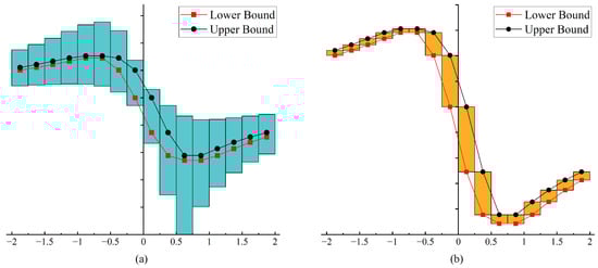
Figure 1.
Bounds predicted by CIA and IIA for : (a) CIA; (b) IIA.
In practical engineering problems, the calculation will lose its application value if the interval result is exaggerated too much. To avoid this phenomenon, the concept of EUI was proposed.
Based on this concept, the i-th interval parameter can be expressed as follows:
where is the EUI associated with the interval parameter , which is used to track the uncertainty of this parameter during the calculation to avoid interval expansion.
For the same function , the bounds predicted using the improved interval algorithm (IIA) are shown in the yellow bar chart in Figure 1b, which are consistent with the exact bounds. Because IIA takes into account the dependence of the interval parameter, the expansion phenomenon caused by the classical interval calculation method can be avoided effectively.
IIA can also be used to improve the accuracy of operations on interval vectors and matrices, where different elements may be affected by the same interval variable.
Similarly, the interval vector is denoted as follows:
where denotes the midpoint of the interval vector; denotes the radius of the interval vector; is the standard interval vector composed of each EUI; and ⊙ represents the Hadamard product, an operation defined only for two matrices and with the same dimension . The result of Hadamard product [36] is also an matrix, whose elements are as follows:
2.2. Interval Finite Element Equation
For the traditional finite element method, the static equilibrium equation of the certain structure can be expressed as follows:
where denotes the global stiffness matrix, which is composed of the element stiffness matrix; is the node displacement vector, whose element is the displacement value of each node of the structure; is the equivalent load vector at the nodes, including load, constraints, and other information of the structure; and d denotes the total number of degrees of freedom of the structure.
In practical engineering structures, parameters such as geometry size or material properties are uncertain, and the uncertainty in the structure can be expressed by interval parameters . Thus, both the structural stiffness matrix and load vector are functions of , and the finite element equilibrium equation can be expressed as follows:
where is the interval vector, composed of each uncertain parameter of the structure; n is the number of uncertain parameters; is the global stiffness matrix considering the structural uncertainty; is the load vector considering the uncertain structure; and is the interval displacement vector to be solved, and its solution set can be described as follows:
The set in Equation (11) is a non-convex polyhedral complex set whose exact features are difficult to obtain.
Finding all possible solutions is of little significance. Therefore, we just care about the upper and lower bounds of the displacement vector . According to Equation (11), the bounds of the interval vector can be defined as follows:
where “max” means to take the maximum value in the set, “min” means to take the minimum value in the set.
3. Adaptive Subinterval Finite Element Method Based on Dynamic Sensitivity Analysis
The solution of interval equilibrium equations is a key step in interval finite element problems. However, traditional interval finite element methods suffer from low accuracy when dealing with problems involving large uncertainties. Although sub-interval methods can improve solution accuracy, they often lead to a significant increase in computational cost. In this section, an improved interval finite element method is introduced as the first step to enhance computational accuracy. Next, expansion routes are constructed based on dynamic sensitivity analysis. Finally, an adaptive strategy is employed to determine an appropriate number of subintervals, and the overall structural response bounds are obtained through interval union operations.
3.1. Improved Interval Finite Element Method
The interval equilibrium equation of Equation (10) is rewritten as an explicit equation:
By using the first-order Taylor series expansion, the stiffness matrix and load vector of the uncertain structure can be expressed as follows:
where and denote midpoints of and , and and denote deviation intervals of and .
The Neumann series expansion [37] is a method used to compute the inverse of a matrix. For an arbitrary matrix , denotes its spectral radius and denotes a unit matrix of the same size as .
If , then exists:
The uncertainty matrix is written in the form of the matrix , whose inverse matrix can be expanded using the Neumann series as follows:
where r is the order of the Neumann expansion and is the inverse matrix of .
Using the above method, the inverse matrix of the interval stiffness matrix can be expanded as follows:
The convergence condition for Equation (18) is as follows:
A sufficient and unnecessary condition for the convergence of the Neumann series expansion is as follows:
For the term in Equation (18), we can convert it to the following explicit form:
If condition is satisfied, the geometric series of the second term converges and can be calculated using the summation formula. Neglecting the non-geometric series terms after the second term, the inverse matrix of the interval stiffness matrix can be approximated as follows:
We write in the above equation as , which is clearly a monotonic function about the interval parameter . Thus, can be expressed in the form of the midpoint and radius as follows:
where
Now, we can express the inverse of the interval stiffness matrix in an explicit form, which facilitates the analysis of a structural uncertainty response.
Substituting Equations (15) and (26) into Equation (13), we can obtain the expression for the displacement vector as follows:
The following symbols are introduced to simplify the writing of Equation (27)
where denotes the midpoint of the interval displacement vector ; denotes the deviation radius of the first-order deviation due to the parameter ; is the second-order deviation determined by the interval parameters and together.
Then, the interval displacement vector can be written as follows:
Now, define the vectors and as follows:
where and correspond to the lower and upper boundaries of the structural response, respectively. Then, substituting and into Equation (29), the upper and lower bounds of the displacement response can be expressed according to IIA as follows:
The interval finite element method proposed in this paper retains a portion of the higher order terms when solving the inverse matrix of the stiffness matrix and considers the second-order deviation terms when solving the displacements. As a result, it is able to obtain more accurate displacement response bounds for the structure than conventional methods such as the first-order truncated Neumann-series-based method [38,39].
3.2. Existing Subinterval Finite Element Method
However, the solution accuracy of the improved interval finite element method is affected by the level of uncertainty. The higher the level of uncertainty, the lower the accuracy of the solution. The subinterval finite element method can be employed when solving the response of structures with large uncertainty.
The uncertainty parameter is divided into subintervals and can be expressed as follows:
where is the -th subinterval of the parameter . The number of subintervals for different parameters can be determined based on its level of uncertainty.
Now, there are a total of subinterval combinations, and each combination can be expressed as follows:
The level of uncertainty for each subinterval is as follows:
Dividing the interval into more subintervals results in lower uncertainty levels for each subinterval. According to interval error estimation theory [40], lower uncertainty levels lead to higher computational accuracy.
Determining the upper and lower bounds of the response for a combination of subintervals is a non-deterministic polynomial (NP)-hard problem. The enumeration method is used to solve this problem. For the subinterval combination , subinterval static equilibrium equations can be written as follows:
Applying the interval finite element method proposed in this paper to each subinterval, the range of displacement responses for each subinterval can be found. For a combination of two adjacent subintervals, the following equation always holds:
For two adjacent subintervals, both the stiffness matrix and load vector have overlapping parts. As a result, the intersection of the interval displacement solutions is not the empty set.
The above equation shows that the displacement solutions of the subintervals can form a single connected region. After solving for the displacement response range of all subintervals, the displacement response range of the interval can be obtained by taking their union as follows:
This method is more accurate than the interval method. However, the subinterval method requires solving the equilibrium equations for all subintervals. When both the dimensionality of the parameters and the number of subintervals are high, the efficiency of this algorithm becomes extremely low due to “combinatorial explosion”.
3.3. Dynamic-Sensitivity-Based Subinterval Finite Element Analysis Method
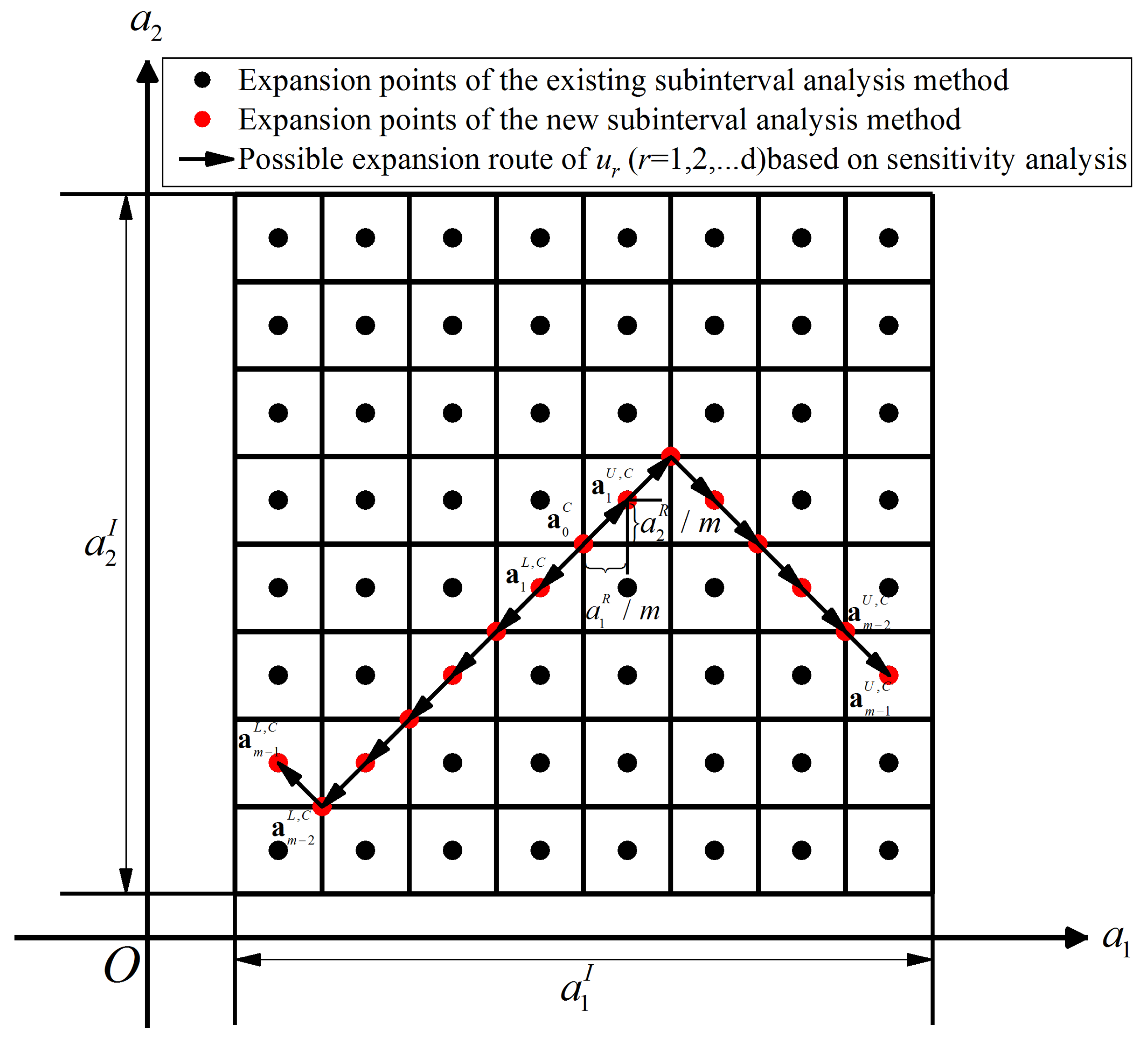
This section proposes an enhanced subinterval method based on dynamic sensitivity analysis in order to improve computational efficiency. A two-dimensional problem is used as an example in order to illustrate the method. The intervals and are divided into subintervals according to the same method. For ease of expression, the number of subintervals for both parameters is taken to be , which can be determined using the adaptive method proposed later.
As shown in Figure 2, the traditional subinterval method requires solving the equilibrium equations for all subintervals. However, in the enhanced subinterval method, only a portion of the subintervals needs to be solved.
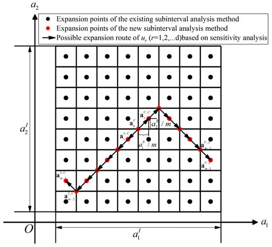
Figure 2.
Possible expansion routes of based on dynamic sensitivity analysis.
For a d-dimensional displacement vector, where each element represents a degree of freedom of the structure, these elements may take on their maximum or minimum values in different combinations of subintervals. Therefore, the interval of the d-th component of the displacement vector is calculated separately in the following. Ultimately, they form the displacement response interval for the entire structure.
First, the finite element equilibrium equation is written for the initial subinterval as follows:
where , represents a subinterval domain and represents an interval vector of the displacement response in the initial subinterval domain .
According to Equation (31), the upper and lower bounds of the displacement interval vectors in the subinterval domain can be obtained.
Then, the displacement interval of the r-th degree of freedom within the subinterval domain can be expressed as follows:
where the subscript r of denotes the r-th degree of freedom of the structure, the subscript 0 denotes the initial subinterval on the expansion route and and denote the r-th element of the vectors and , respectively.
To avoid solving for all the intervals, a natural idea is to find an expansion route such that the bounds of can be predicted by solving the equilibrium equations on it. To predict the upper bound of the displacement response , the subinterval should move in the direction that makes it increase. Conversely, to predict the lower bound of the displacement response , the subinterval should move in the direction that makes it decrease. Therefore, the new vectors and are formed of the r-th element of the vector sequences and , respectively. The superscript L indicates that this vector is used to determine the lower displacement bounds, and the superscript U indicates that this vector is used to determine the upper displacement bounds. The meanings of L and U are the same in the latter part of the paper. Then, the midpoints of the next subintervals on the expansion routes of the upper and lower bounds of can be represented, respectively, as follows:
The next subintervals on the expansion routes of the upper and lower bounds of can be expressed, respectively, as follows:
By solving the interval equilibrium equations for the two subinterval domains and using Equations (28)–(31), we can obtain the interval displacement vectors and as follows:
The interval of the r-th displacement component in the subinterval domains and can be expressed as follows:
Meanwhile, the sensitivity vector sequences and in the subintervals and domains can be obtained according to Equation (30).
The r-th elements of the vector sequences and are extracted, forming two vectors:
The positions of the next expansion points on the routes of the upper and lower bounds of can be obtained using these two vectors.
By repeating the above process m − 1 times, a series midpoints points and of subintervals and can be determined:
In subintervals and , the equilibrium equations are solved using Equations (28)–(31), respectively. The interval in subinterval domains and in subinterval domains of the displacement component can be obtained.
Due to
Thus,
Via a union operation, the lower bound of and upper bound of can be represented as follows:
Theoretically, if the expansion routes are not chosen, there are a total of possible combinations of subintervals. According to Equation (50), moves in the decreasing direction of , and moves in the increasing direction of . Thus, based on dynamic sensitivity analysis, we can obtain the following relationship:
Similarly,
By employing the aforementioned method, the lower and upper bounds and for each displacement component are obtained, and they are combined to form the bounds of displacement vector. It is important to note that there is no need to repeat the calculation for the same expansion point on different expansion routes. If interval finite element analysis has already been performed within a certain subinterval domain, the previous results can be directly utilized.
3.4. An Adaptive Convergence Mechanism and Computational Procedure
Clearly, in the proposed subinterval finite element method, the accuracy increases with the number of subintervals. However, the computational cost of this method also increases. It is desirable to use as few subintervals as possible while still satisfying the accuracy. Therefore, an adaptive convergence mechanism is proposed to determine the appropriate number of subintervals.
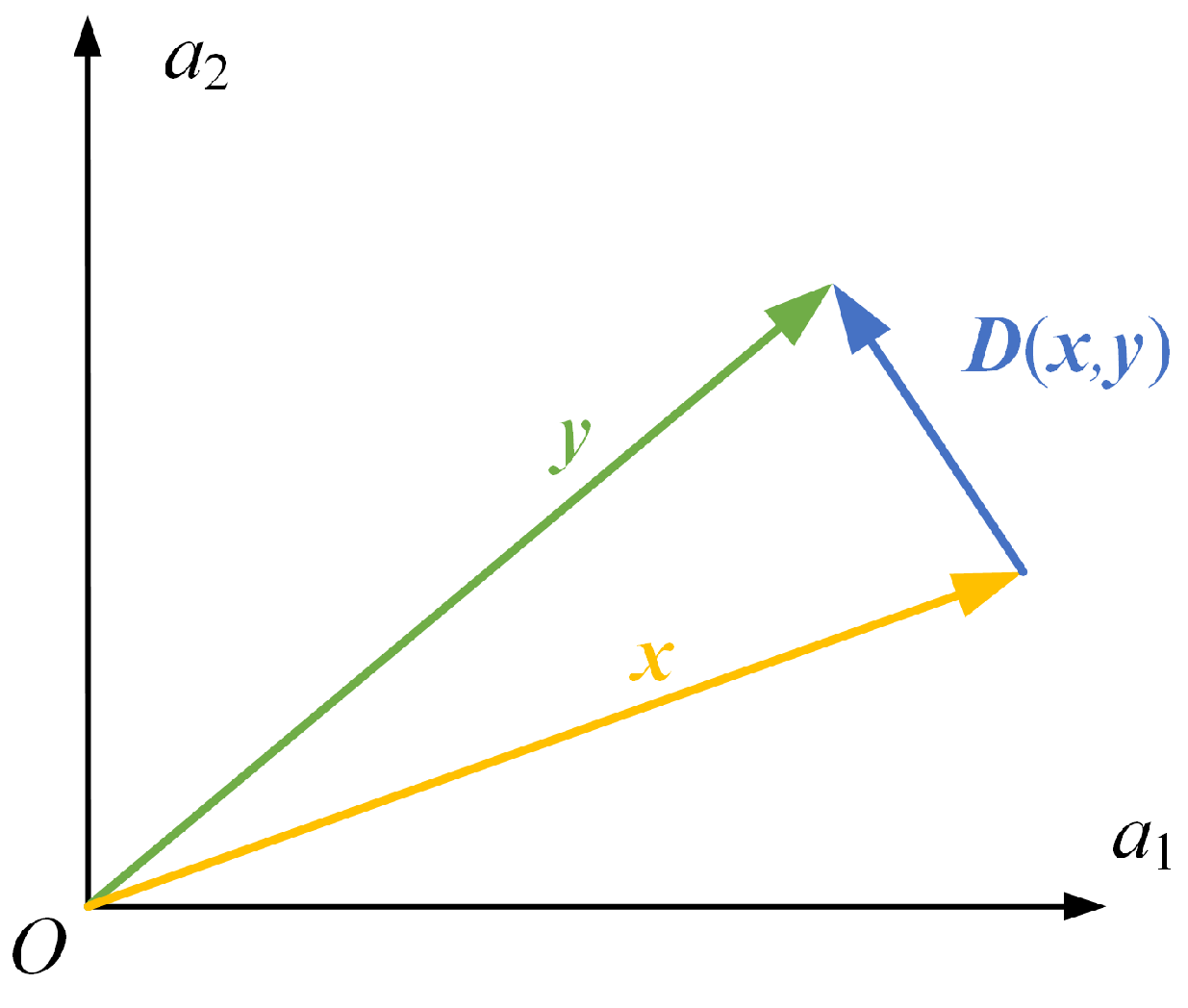
We propose a method to evaluate the relative error of vectors. For the vector to be compared and the known vector , the relative error can be defined as follows:
where is the 2-norm of vectors and is the Euclidean distance of from .
The relative error between two 2D vectors can be expressed as shown in Figure 3.
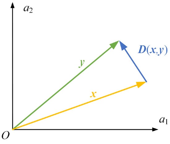
Figure 3.
Definition of the relative error between vectors (2D vectors for example).
Therefore, the computational process of the dynamic sensitivity-based subinterval finite element method includes the following steps:
- (1)
- Set and .
- (2)
- Solve the upper and lower bounds of the displacement in the original interval, noted as and .
- (3)
- Set and , and then, divide each interval into m subintervals.
- (4)
- Find the upper bound and lower bound using the subinterval finite element method based on dynamic sensitivity analysis and assemble them as and .
- (5)
- Calculate the iteration error .
- (6)
- If is not larger than the permissible error , output and as the upper and lower bounds of the structural displacement response. Otherwise, return to the third step.
The calculation process of the dynamic-sensitivity-based subinterval finite element method is shown in Figure 4. Through this process, it is possible to obtain the upper and lower limits of the structural displacement response with relatively few iterations.
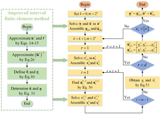
Figure 4.
Flowchart of adaptive subinterval finite element method based on dynamic sensitivity analysis.
4. Applications
In this section, two examples are given to demonstrate the accuracy and efficiency of the proposed method (PM) for solving uncertain structures. The displacement response bounds of the nine-bar truss and the impeller were computed. For comparison purposes, the results obtained using the vertex method or the scanning method are used as reference solutions. The subinterval decomposition analysis method (SDAM) [14] and the STM are also used to calculate the response bounds for comparison. The error of the obtained results is defined and computed as follows:
The errors of all methods in this paper are based on the accuracy of the numerical calculations.
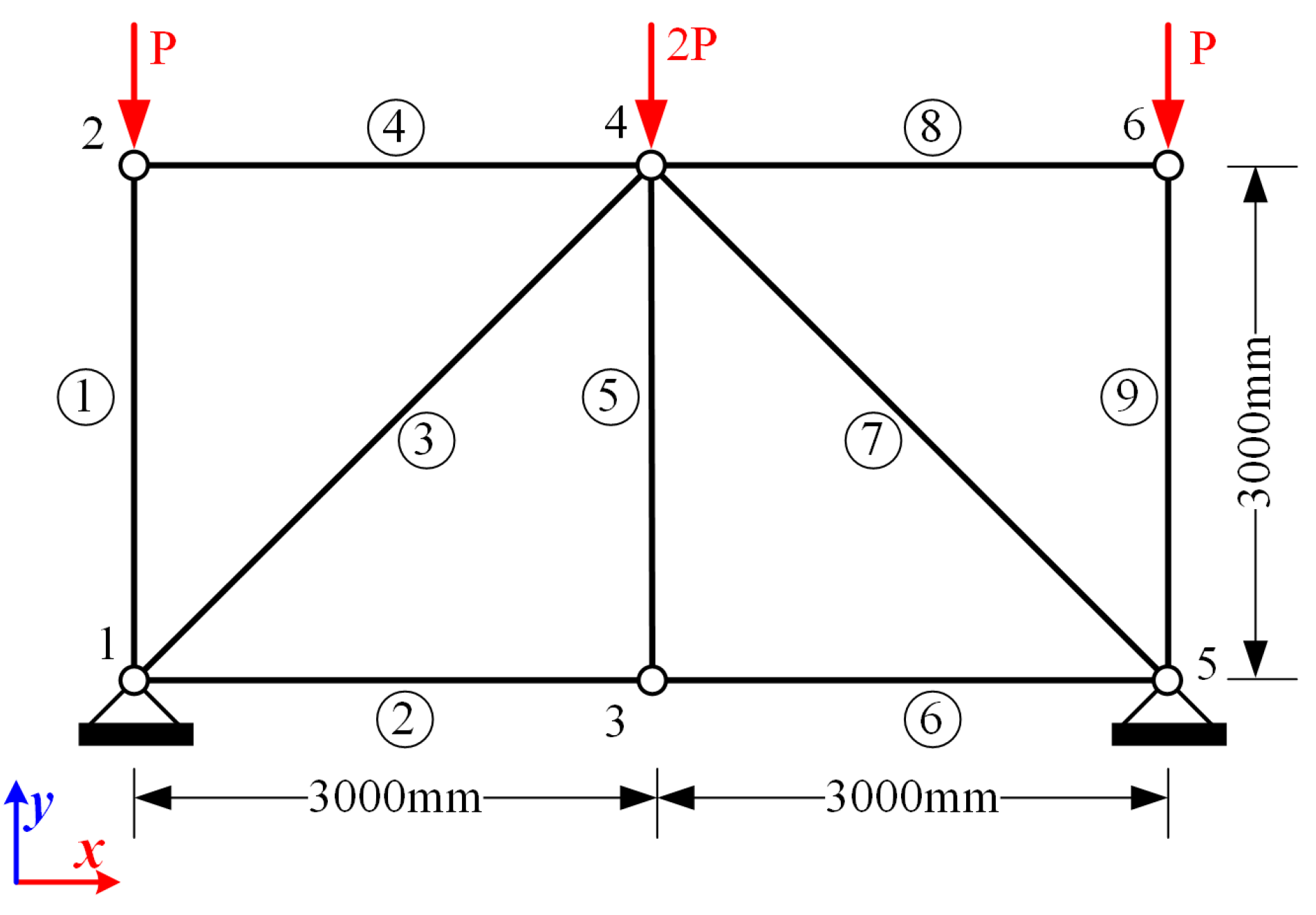
4.1. Nine-Bar Truss
A nine-bar 2D truss structure is shown in Figure 5. The height and span of the truss structure are 3 m and 6 m, respectively. The total number of elements is nine, and the total number of nodes is six. The horizontal and vertical displacements of node 1 and node 5 are constrained. The vertical loads shown in Figure 5 are applied to nodes 2, 4, and 6. In this example, the Young’s modulus and cross-sectional area of each bar, as well as the load, are considered as independent interval parameters. Therefore, they are defined according to Equation (58):
where and are the uncertainty levels for Young’s modulus and the cross-sectional area of each rod (), and is the uncertainty level of the load P.
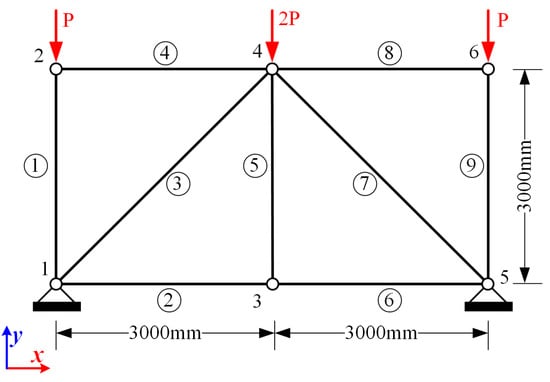
Figure 5.
Nine-bar truss structure.
Three cases are considered and the level of uncertainty in each case is shown in Table 1. Simulations of this nine-bar truss are carried out using MATLAB R2018b on a computer with a 2.90 GHz AMD Ryzen 7 CPU and 16.0 GB RAM.

Table 1.
Uncertainty levels of interval parameters for the nine-bar truss in three cases.
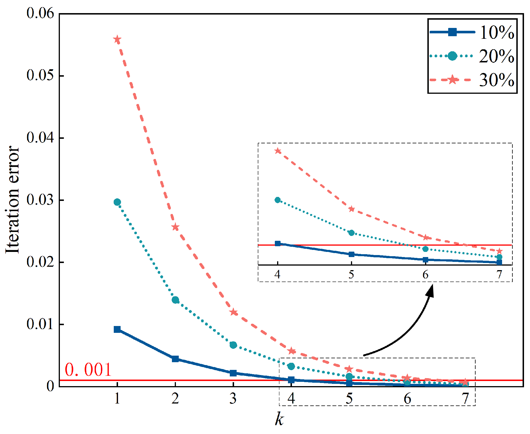
The levels of uncertainty for all interval variables in the first two cases are 10% and 20%, respectively. Then, the level of uncertainty is set to 30% in case 3 to illustrate the advantages of the proposed method when dealing with large levels of uncertainty. In each case, the upper and lower bounds of the displacement are solved using VM, SDAM, STM, and the PM. The results of VM are used as the reference solution. In order to investigate the influence of on the accuracy and efficiency of the proposed method, different convergence values (=1%, 5‰, 1‰) were considered for the calculations. The upper and lower bounds and errors of the node displacements (x displacement for node 2 and y displacement for node 4) obtained using different methods are presented in Table 2 and Table 3. The calculation times for the different methods at the 30% uncertainty level are shown in Table 4. Iterative error curves for structural displacements at the 10%, 20%, and 30% uncertainty levels are given in Figure 6.
Table 2.
Bounds and errors of for the three cases.
Table 3.
Bounds and errors of for the three cases.
Table 4.
The calculation times for the different methods at the 30% uncertainty level.
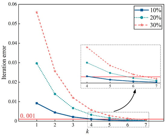
Figure 6.
Iterative error curves of overall structural displacements of the nine-bar truss for the three cases.
To examine the influence of the uncertainty levels on the accuracy of each method, further computations were conducted for varying uncertainty levels of the structural response. The uncertainty levels of all interval parameters were incrementally increased from 0 to 30% with an increment of 1%. The upper and lower bound curves of the displacements determined using VM, SDAM, STM, and the PM at different levels of uncertainty are plotted in Figure 7.
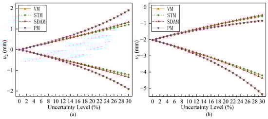
Figure 7.
Bounds of nodal displacements of the nine-bar truss obtained using the different methods: (a) x-displacement ; (b) y-displacement .
By analyzing the results obtained from different methods, the following conclusions can be drawn:
- (1)
- As can be seen from Table 4, the calculation time for the PM is much less than that of VM, despite the fact that the permissible error for the PM is as small as 1‰. For VM, the equilibrium equation needs to be solved for all the possible combinations of intervals. Thus, the computational cost is exponentially related to the number of interval parameters. Such large computational costs are unacceptable, especially for structures containing many interval parameters. However, for the PM, the computational cost is much less than that of VM because the equilibrium equations only need to be solved at specific points. Therefore, the PM can be applied to interval finite element analysis with a large number of uncertain parameters and retains sufficient computational efficiency.
- (2)
- As expected, the errors for these interval analysis methods in Figure 7 all increase as the level of uncertainty rises. However, the calculations show that the displacement response bounds solved by the PM are more accurate than the other two methods. When the uncertainty level reaches 30%, the maximum errors for SDAM and STM reach 42.43% and 36.31%, respectively, while the maximum error for the PM is only 0.28%. Therefore, the PM is suitable for analyzing the displacement response of structures under high levels of uncertainty.
- (3)
- For all three cases, the iteration error gradually decreases. Until the iteration error decreases below the permissible error , suitable computational results are obtained. Case 1 and case 2 require only five and six iterations, respectively, whereas case 3 requires seven iterations. This suggests that the number of iterations of the PM gradually increases as the uncertainty of the structure rises.
4.2. Impeller
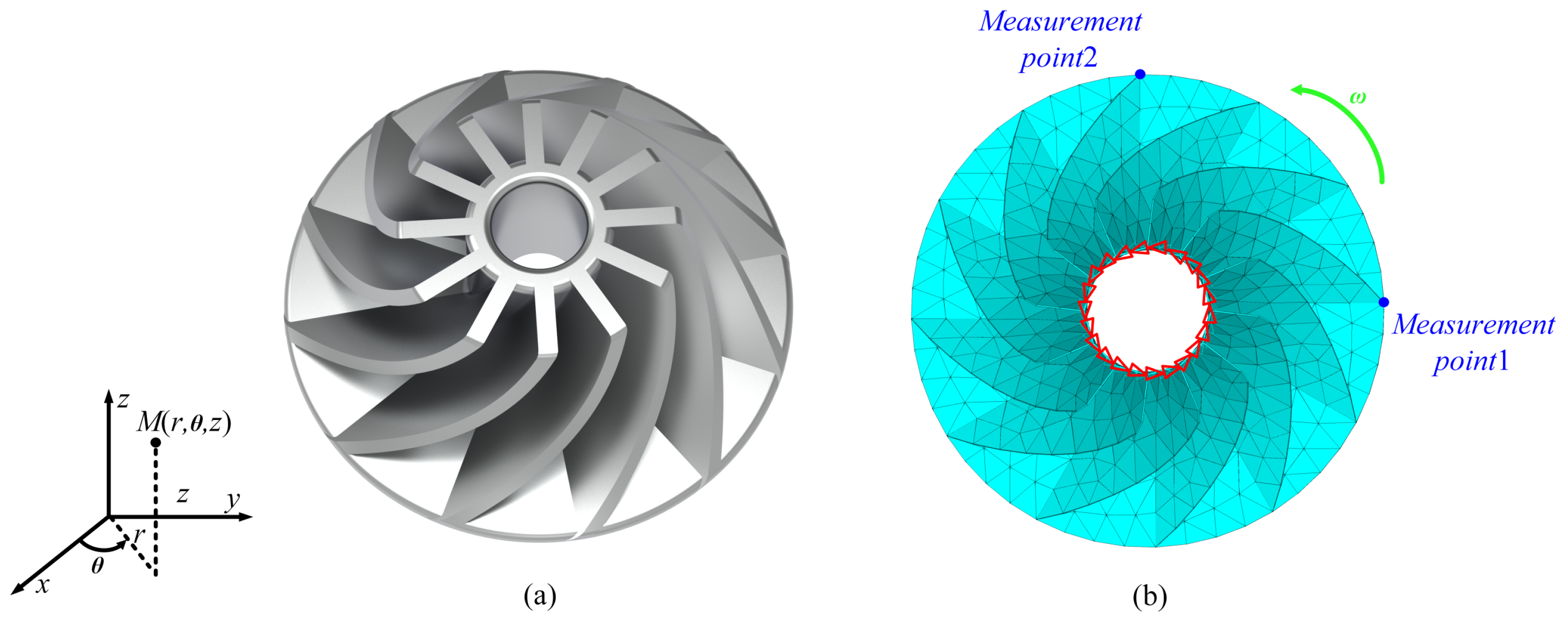
The second example analyzes the response of an impeller, as shown in Figure 8a, to demonstrate the efficiency and accuracy advantages of the proposed method. The material of the impeller is carbon steel, with density and Young’s modulus being and E, respectively. A shell element model is established as shown in Figure 8b, with a thickness t. Considering the unpredictability of material properties and manufacturing processes, , E, and t are treated as independent interval variables. The tangential and longitudinal degrees of freedom at the nodes on the impeller sleeve are constrained, as illustrated in Figure 8b. The angular velocity of the structure, denoted as , is also an uncertain-but-bounded parameter. This example also considers three uncertainty cases and the median values of all uncertain parameters are shown in Table 5.
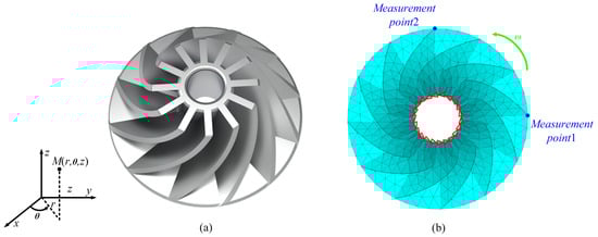
Figure 8.
Impeller structure: (a) geometric model; (b) finite element model.
Table 5.
Median values of interval parameters of impeller structure.
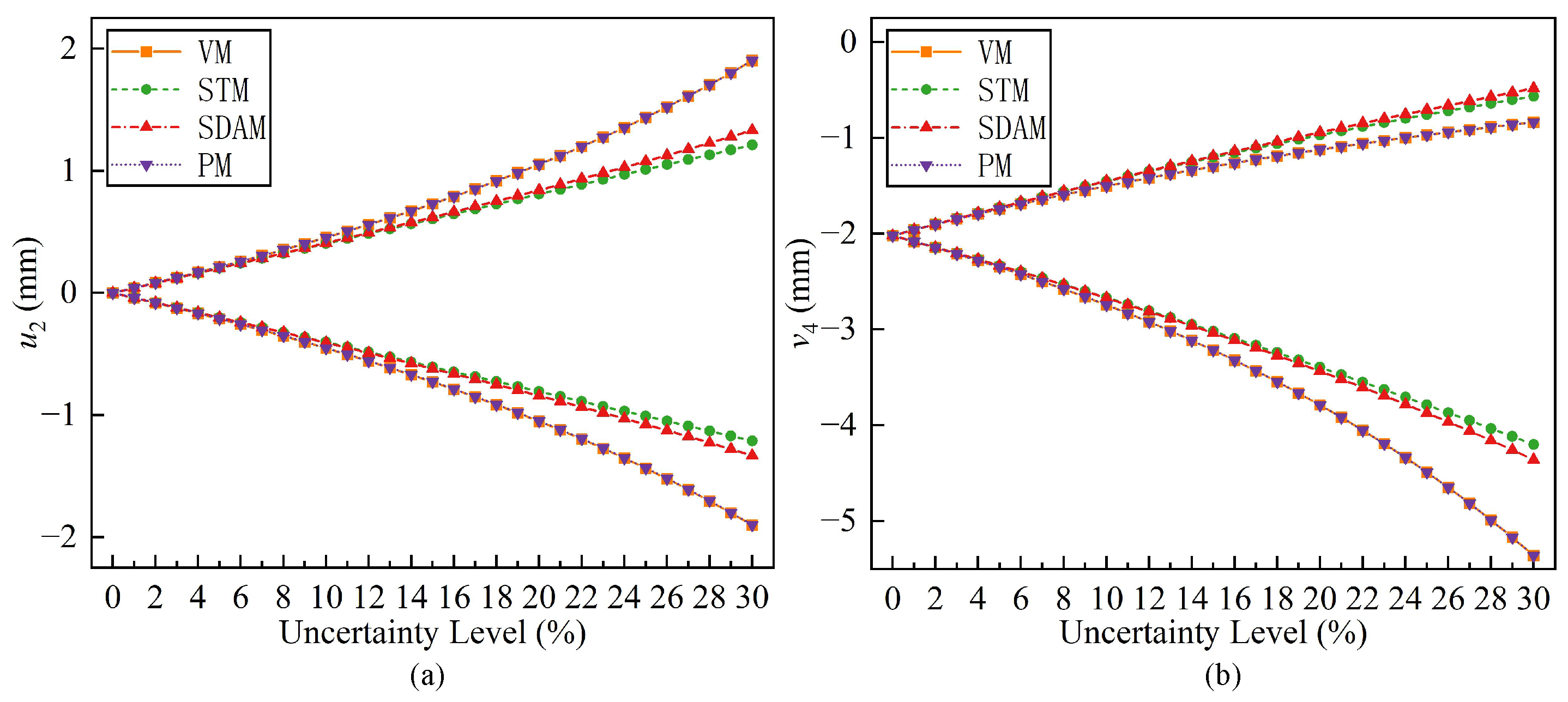
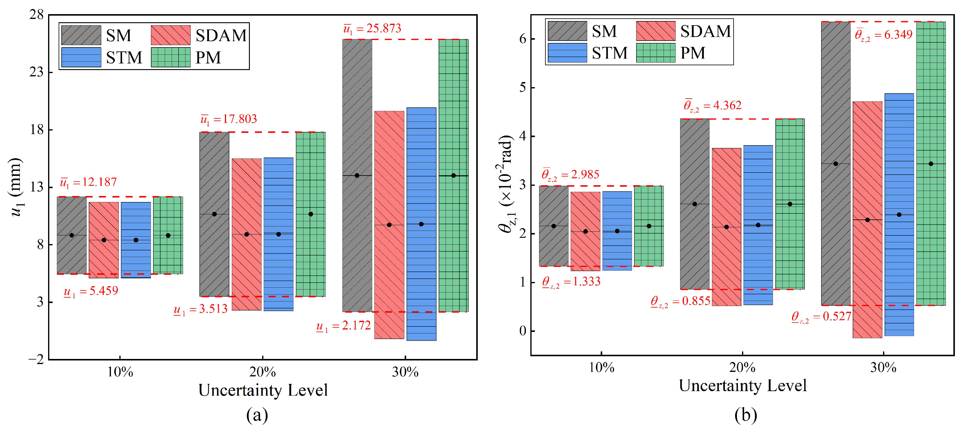
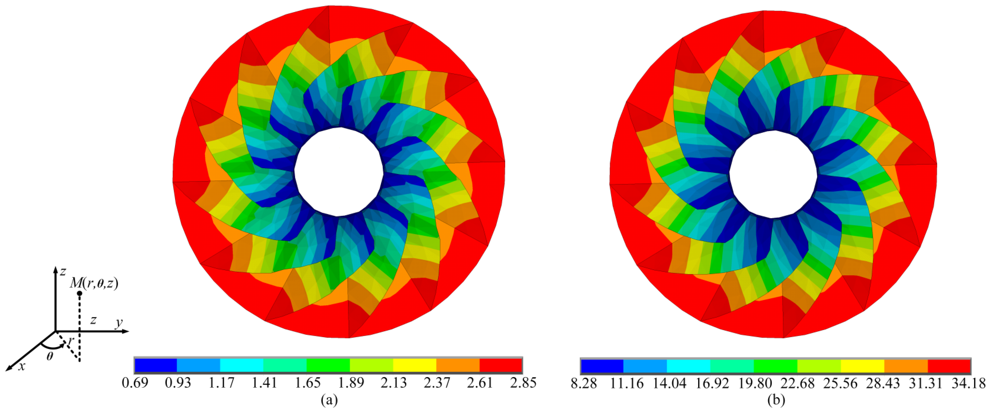
To observe the displacement variation in the impeller, two nodes were selected as measurement points, as shown in Figure 8b. The upper and lower bounds of the displacement and rotation at the measurement points were computed for different uncertainty levels. Case 1 sets the uncertainty level at 10% for all interval parameters, while cases 2 and 3 extend the uncertainty level to 20% and 30%, respectively. The bounds of displacements and rotations obtained using the PM are compared with those of SDAM and STM, and the solutions obtained by SM are used as references. The bounds and errors for the nodal displacements and rotations (x-component of the displacement of node 1 and z-component of the rotation of node 2 ) calculated with different methods for each uncertainty case are given in Table 6 and Table 7. In addition, the upper and lower bounds of the nodal displacements and rotations obtained using the different methods are plotted in Figure 9. In Figure 10, the overall structural displacement bound cloud maps for the impeller obtained using the PM at the 30% uncertainty level are given.
Table 6.
Bounds and errors of for the three cases.
Table 7.
Bounds and errors of for the three cases.

Figure 9.
Bounds of nodal displacements of the impeller obtained using the different methods: (a) x-component of displacement of node 1 ; (b) z-component of rotation of node 2 .

Figure 10.
Structural displacement bound clouds for impeller: (a) lower bound; (b) upper bound.
As shown in Table 6 and Table 7 and Figure 9 and Figure 10, the second numerical example shows that the PM is still accurate and efficient for impeller structure.
- (1)
- The response bounds obtained for SDAM, STM, and the PM have a tendency to increase with the level of uncertainty rising. When the uncertainty level reaches 30%, the maximum errors for SDAM are −119.06% and those for STM are −127.33%. However, the error of the results obtained using the PM does not exceed 1%. Although the PM only retains the first-order term of the Taylor expansion, its accuracy is higher than STM, which retains the second-order term. There are two main reasons for this: Firstly, the PM utilizes a modified Neumann series, which retains higher-order terms of the Neumann series. Secondly, the PM divides the interval into subintervals, reducing the uncertainty level during the solving process. The reason why the PM is more accurate than SDAM is that SDAM only expands at the midpoint of the interval to approximate the response at the combination point, while the PM solves within the subinterval domains of each expansion route.
- (2)
- PM is still suitable for finite element models with high levels of uncertainty and multiple parameters and can maintain good efficiency. The computational effort of SM increases exponentially with the number of parameters, which makes it limited when the number of interval parameters is large. However, the cost of computation is significantly reduced when using PM because it only needs to solve the equilibrium equations along the expansion routes.
- (3)
- According to Figure 9, increasing the uncertainty of interval parameters leads to the expansion of the response interval. This indicates that the extreme conditions of the structure can only be predicted when uncertainty is taken into account. Design solutions obtained by considering uncertainty are more secure and reliable.
5. Conclusions
A novel adaptive subinterval finite element method based on dynamic sensitivity analysis is proposed in this paper to predict the displacement response bounds of structures under static loads with uncertain-but-bounded parameters. The proposed method is efficient since the equilibrium equations need to be solved at only a few subinterval sets selected by the constructed expansion routes. And, the proposed method has high accuracy since the Neumann series and interval algorithm were improved. Compared with methods based on the first-order truncated Neumann series, the improved Neumann series method retains some high-order terms. The interval expansion due to the dependence phenomenon is effectively avoided by the improved interval algorithm. The proposed method is compared with other interval analysis methods. Through the numerical example analyses, it is found that the results of the proposed subinterval analysis method are very close to the reference solutions; the efficiency is greatly improved when compared with the vertex combination method and the scanning method; the accuracy is better than the subinterval decomposition analysis method and the second-order Taylor expansion-based method. In the future, the proposed method can potentially be extended to predict response intervals for multi-field coupled problems.
Author Contributions
Conceptualization, M.H.; Methodology, G.Y.; Software, K.G.; Validation, M.H., K.G. and M.W.; Resources, G.Y.; Data curation, M.H.; Funding acquisition, M.W.; Writing—original draft preparation, M.H. and K.G.; Writing—review and editing, M.H. and K.G. All authors have read and agreed to the published version of the manuscript.
Funding
This work is supported by the “Research on development strategy and technical path of high-temperature superconducting maglev transportation (2019-JL-7)” (key consulting projects of the Chinese Academy of Engineering) and the “Research on systematic technology of maglev transportation (2020CKA002)” (major scientific research projects of the CRRC), as well as the “Research and verification of key technologies of high-temperature super-conductive maglev trains with speeds of 600 kmph (2021CCZ002-2)”.
Institutional Review Board Statement
Not applicable.
Informed Consent Statement
Not applicable.
Data Availability Statement
The data that support the findings of this study are available from the corresponding author upon reasonable request.
Acknowledgments
The authors thank the Department of Mechanics of Jilin University for supporting this research. The authors also thank the editors for their efforts and the reviewers for their valuable suggestions.
Conflicts of Interest
The authors declare no conflict of interest.
References
- Fu, Z.; Tian, L.; Liu, J. Seismic response and collapse analysis of a transmission tower-line system considering uncertainty factors. J. Constr. Steel Res. 2022, 189, 107094. [Google Scholar] [CrossRef]
- Fu, C.; Sinou, J.J.; Zhu, W.; Lu, K.; Yang, Y. A state-of-the-art review on uncertainty analysis of rotor systems. Mech. Syst. Signal Process. 2023, 183, 109619. [Google Scholar] [CrossRef]
- Tang, Z.; Li, W.; Zhou, S.; Sun, J. Research on Railway Emergency Resources Scheduling Model under Multiple Uncertainties. Appl. Sci. 2023, 13, 4432. [Google Scholar] [CrossRef]
- Zhou, X.; Sun, Y.; Xiao, H. Simulation of Cross-Correlated Random Fields for Transversely Anisotropic Soil Slope by Copulas. Appl. Sci. 2023, 13, 4234. [Google Scholar] [CrossRef]
- Yang, Z.; Huang, J.; Yang, D.; Zhong, Z. Design and optimization of robust path tracking control for autonomous vehicles with fuzzy uncertainty. IEEE Trans. Fuzzy Syst. 2021, 30, 1788–1800. [Google Scholar] [CrossRef]
- Łasecka Plura, M. Dynamic Characteristics of a Composite Beam with Viscoelastic Layers under Uncertain-but-Bounded Design Parameters. Appl. Sci. 2023, 13, 6473. [Google Scholar] [CrossRef]
- Ma, J.; Fu, C.; Zheng, Z.; Lu, K.; Yang, Y. The Effects of Interval Uncertainties on Dynamic Characteristics of a Rotor System Supported by Oil-Film Bearings. Lubricants 2022, 10, 354. [Google Scholar] [CrossRef]
- Moore, R.E. Interval Analysis; Prentice-Hall: Englewood Cliffs, NJ, USA, 1966; Volume 4. [Google Scholar]
- Alefeld, G.; Herzberger, J. Introduction to Interval Computation; Academic Press: Cambridge, MA, USA, 2012. [Google Scholar]
- Long, X.; Jiang, C.; Han, X.; Tang, J.; Guan, F. An enhanced subinterval analysis method for uncertain structural problems. Appl. Math. Model. 2018, 54, 580–593. [Google Scholar] [CrossRef]
- Muhanna, R.L.; Zhang, H.; Mullen, R.L. Interval finite elements as a basis for generalized models of uncertainty in engineering mechanics. Reliab. Comput. 2007, 13, 173–194. [Google Scholar] [CrossRef]
- Chen, S.H.; Yang, X.W. Interval finite element method for beam structures. Finite Elem. Anal. Des. 2000, 34, 75–88. [Google Scholar] [CrossRef]
- Fu, C.; Zheng, Z.; Zhu, W.; Lu, K.; Yang, Y. Non-intrusive frequency response analysis of nonlinear systems with interval uncertainty: A comparative study. Chaos Solitons Fractals 2022, 165, 112815. [Google Scholar] [CrossRef]
- Fu, C.; Cao, L.; Tang, J.; Long, X. A subinterval decomposition analysis method for uncertain structures with large uncertainty parameters. Comput. Struct. 2018, 197, 58–69. [Google Scholar] [CrossRef]
- Rao, S.S.; Berke, L. Analysis of uncertain structural systems using interval analysis. AIAA J. 1997, 35, 727–735. [Google Scholar] [CrossRef]
- Wu, J.; Zhang, Y.; Chen, L.; Luo, Z. A Chebyshev interval method for nonlinear dynamic systems under uncertainty. Appl. Math. Model. 2013, 37, 4578–4591. [Google Scholar] [CrossRef]
- Fu, C.; Yang, Y.; Lu, K.; Gu, F. Nonlinear vibration analysis of a rotor system with parallel and angular misalignments under uncertainty via a Legendre collocation approach. Int. J. Mech. Mater. Des. 2020, 16, 557–568. [Google Scholar] [CrossRef]
- Zheng, Y.; Qiu, Z. Uncertainty propagation in aerodynamic forces and heating analysis for hypersonic vehicles with uncertain-but-bounded geometric parameters. Aerosp. Sci. Technol. 2018, 77, 11–24. [Google Scholar] [CrossRef]
- Liu, Y.; Wang, X.; Wang, L.; Lv, Z. A Bayesian collocation method for static analysis of structures with unknown-but-bounded uncertainties. Comput. Methods Appl. Mech. Eng. 2019, 346, 727–745. [Google Scholar] [CrossRef]
- De, S.; Maute, K.; Doostan, A. Bi-fidelity stochastic gradient descent for structural optimization under uncertainty. Comput. Mech. 2020, 66, 745–771. [Google Scholar] [CrossRef]
- Qiu, Z.; Zhu, B. A Newton iteration-based interval analysis method for nonlinear structural systems with uncertain-but-bounded parameters. Int. J. Numer. Methods Eng. 2021, 122, 4922–4943. [Google Scholar] [CrossRef]
- Dinh-Cong, D.; Van Hoa, N.; Nguyen-Thoi, T. An effective optimization-based parameterized interval analysis approach for static structural response with multiple uncertain parameters. Eng. Comput. 2020, 36, 1889–1902. [Google Scholar] [CrossRef]
- Kabir, H.D.; Khosravi, A.; Hosen, M.A.; Nahavandi, S. Neural network-based uncertainty quantification: A survey of methodologies and applications. IEEE Access 2018, 6, 36218–36234. [Google Scholar] [CrossRef]
- Wang, L.; Liu, Y.; Gu, K.; Wu, T. A radial basis function artificial neural network (RBF ANN) based method for uncertain distributed force reconstruction considering signal noises and material dispersion. Comput. Methods Appl. Mech. Eng. 2020, 364, 112954. [Google Scholar] [CrossRef]
- Abdullah, A.A.; Hassan, M.M.; Mustafa, Y.T. Uncertainty Quantification for MLP-Mixer Using Bayesian Deep Learning. Appl. Sci. 2023, 13, 4547. [Google Scholar] [CrossRef]
- Qiu, Z.; Chen, S.; Elishakoff, I. Bounds of eigenvalues for structures with an interval description of uncertain-but-non-random parameters. Chaos Solitons Fractals 1996, 7, 425–434. [Google Scholar] [CrossRef]
- Xia, B.; Yu, D. Interval analysis of acoustic field with uncertain-but-bounded parameters. Comput. Struct. 2012, 112, 235–244. [Google Scholar] [CrossRef]
- Wu, F.; Gong, M.; Ji, J.; Peng, G.; Yao, L.; Li, Y.; Zeng, W. Interval and subinterval perturbation finite element-boundary element method for low-frequency uncertain analysis of structural-acoustic systems. J. Sound Vib. 2019, 462, 114939. [Google Scholar] [CrossRef]
- Wang, C.; Qiu, Z. Modified perturbation method for eigenvalues of structure with interval parameters. Sci. China Physics, Mech. Astron. 2015, 58, 1–9. [Google Scholar] [CrossRef]
- Moore, R.E.; Kearfott, R.B.; Cloud, M.J. Introduction to Interval Analysis; SIAM: Philadelphia, PA, USA, 2009. [Google Scholar]
- Degrauwe, D.; Lombaert, G.; De Roeck, G. Improving interval analysis in finite element calculations by means of affine arithmetic. Comput. Struct. 2010, 88, 247–254. [Google Scholar] [CrossRef]
- Sofi, A.; Romeo, E. A novel interval finite element method based on the improved interval analysis. Comput. Methods Appl. Mech. Eng. 2016, 311, 671–697. [Google Scholar] [CrossRef]
- Sofi, A.; Romeo, E.; Barrera, O.; Cocks, A. An interval finite element method for the analysis of structures with spatially varying uncertainties. Adv. Eng. Softw. 2019, 128, 1–19. [Google Scholar] [CrossRef]
- Chen, S.H.; Ma, L.; Meng, G.W.; Guo, R. An efficient method for evaluating the natural frequencies of structures with uncertain-but-bounded parameters. Comput. Struct. 2009, 87, 582–590. [Google Scholar] [CrossRef]
- Xia, B.; Yu, D. Modified interval and subinterval perturbation methods for the static response analysis of structures with interval parameters. J. Struct. Eng. 2014, 140, 04013113. [Google Scholar] [CrossRef]
- Horn, R.A. The hadamard product. Proc. Symp. Appl. Math 1990, 40, 87–169. [Google Scholar]
- Wu, M.; Yin, B.; Vosoughi, A.; Studer, C.; Cavallaro, J.R.; Dick, C. Approximate matrix inversion for high-throughput data detection in the large-scale MIMO uplink. In Proceedings of the 2013 IEEE International Symposium on Circuits and Systems (ISCAS), Beijing, China, 19–23 May 2013; pp. 2155–2158. [Google Scholar]
- Chen, S.; Lian, H.; Yang, X. Interval static displacement analysis for structures with interval parameters. Int. J. Numer. Methods Eng. 2002, 53, 393–407. [Google Scholar] [CrossRef]
- Wu, F.; Gong, M.; Yao, L.; Hu, M.; Jie, J. High precision interval analysis of the frequency response of structural-acoustic systems with uncertain-but-bounded parameters. Eng. Anal. Bound. Elem. 2020, 119, 190–202. [Google Scholar] [CrossRef]
- Zhou, Y.; Jiang, C.; Han, X. Interval and subinterval analysis methods of the structural analysis and their error estimations. Int. J. Comput. Methods 2006, 3, 229–244. [Google Scholar] [CrossRef]


Disclaimer/Publisher’s Note: The statements, opinions and data contained in all publications are solely those of the individual author(s) and contributor(s) and not of MDPI and/or the editor(s). MDPI and/or the editor(s) disclaim responsibility for any injury to people or property resulting from any ideas, methods, instructions or products referred to in the content. |
© 2023 by the authors. Licensee MDPI, Basel, Switzerland. This article is an open access article distributed under the terms and conditions of the Creative Commons Attribution (CC BY) license (https://creativecommons.org/licenses/by/4.0/).