Analysis of Kinematic Constraints in the Linkage Model of a Mecanum-Wheeled Robot and a Trailer with Conventional Wheels

Abstract

Mechanical systems that consist of a four-wheeled or two-wheeled robot with Mecanum wheels and a two-wheeled trailer with conventional wheels are considered. The kinematic characteristics of the mechanical systems under consideration of holonomic and non-holonomic constraints are presented and compared. From this, it is shown that the structure of the kinematic constraint equations for mobile systems with a trailer does not apply to Chaplygin’s dynamic equations. If the mechanical system is not Chaplygin’s system, then the dynamic equations cannot be integrated separately from the equations of kinematic constraints. This is the difference between the kinematic constraint equations for the robot-trailer system and the constraint equations for a single robot with Mecanum wheels. Examples of numerical calculations using the equations of kinematic constraints are given.

1. Introduction

For over a hundred years, engineers have been developing wheels that allow moving not only in the plane of a wheel but also in the direction perpendicular to this plane. Such developments originated from an invention by J. Grabowiecki, which was patented in the USA in 1919 [1].

Robots with Mecanum wheels are being intensively studied because the design of such wheels allows the robots to maneuver in a highly constrained environment, e.g., in warehouses [2,3,4,5,6]. Mobile robots with Mecanum wheel can move in any direction and perform both translations and rotations. A Mecanum wheel has the rollers arranged uniformly along the circumference of the wheel in such a way that the axes of rotation of the rollers form the same angle with the wheel’s plane; per definition, this angle equals 45°. Many different studies and research groups are dealing with the kinematics and dynamics of robots with Mecanum wheels. A robot with Mecanum wheels and the possibility of height and width adaptation is discussed in [7,8]. The kinematic constraints for systems with such wheels are considered in [9,10,11,12,13,14,15,16], for instance. If the contact of the wheel with the underlying surface occurs at a point and the wheel is rolling without slip, the respective kinematic constraints are non-holonomic. The system with non-holonomic constraints should be treated with appropriate non-holonomic mechanical techniques [17,18,19]. Lagrange’s equations of the second kind apply only to mechanical systems with holonomic constraints and thus cannot be applied to robots with Mecanum wheels as mistakenly published in [20]. The kinematics and dynamics of a mobile platform with four Mecanum wheels are addressed in detail in [21,22,23,24]. These studies present different techniques for solving the kinematic constraint equations and establish relations among them. The structure of the constraint equations for a four-wheeled robot with Mecanum wheels allows using Chaplygin’s equations as the governing dynamic equations. These equations allow solving the dynamic equations separately from the constraint equations, which significantly simplifies the problem [25].

In our paper, we consider the kinematic constraint equations for systems that consist of a two-wheeled or four-wheeled robot with Mecanum wheels and a two-wheeled trailer with conventional wheels. The structure of the kinematic equations for the robot-trailer system is essentially different from the structure of the kinematic equations for a single robot, which should be taken into account when deriving the dynamic equations.

2. Kinematic Constraint Equations

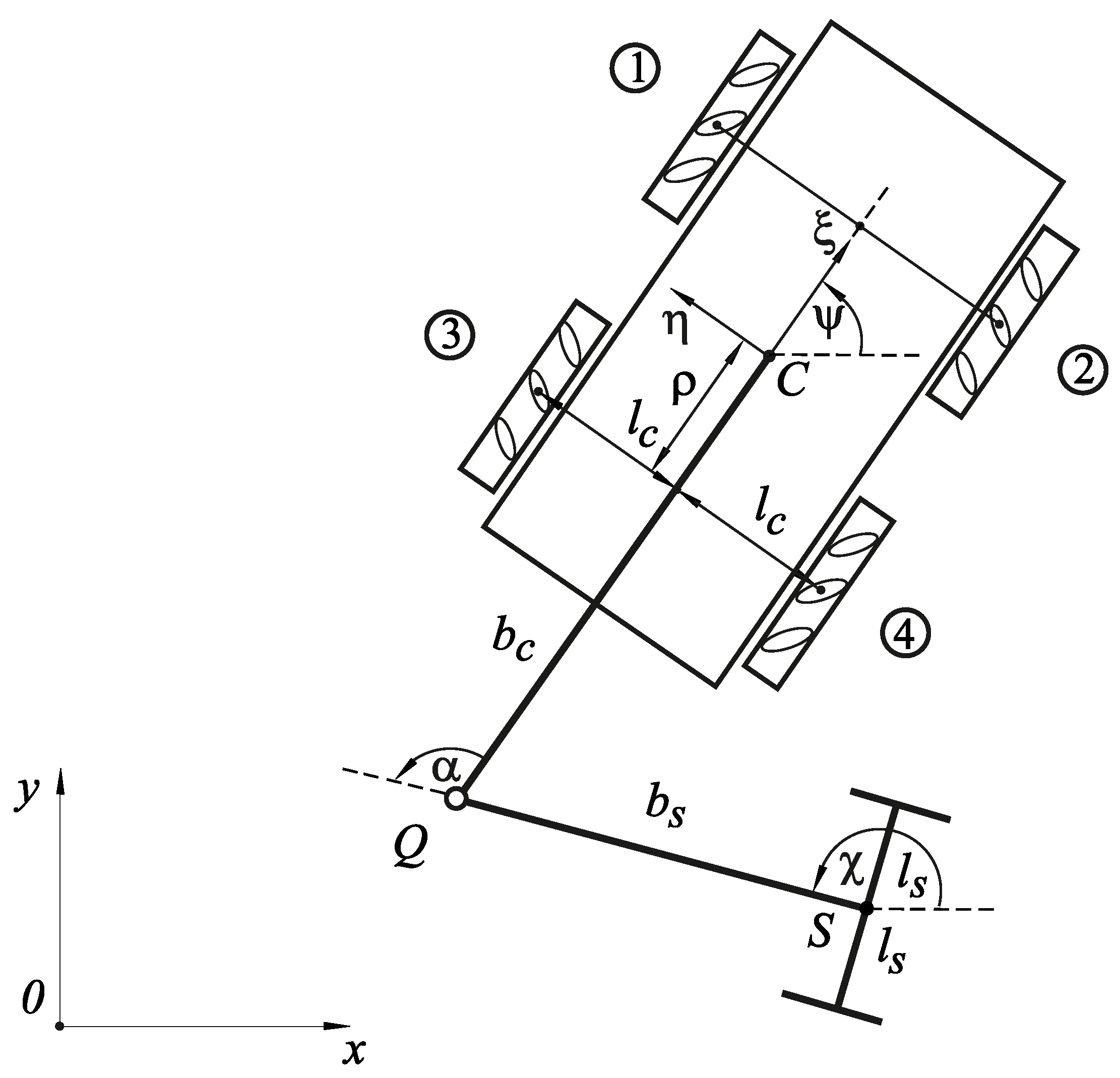
A robot-trailer system consists of a four- or two-wheeled robot with Mecanum wheels and a two-wheeled trailer with conventional wheels located on one axis. All wheels of the robot-trailer system have permanent contact with the surface.

The center of mass C is on the longitudinal axis of the robot’s body so that the track width is $2l_C$. The quantity $\rho$ denotes the distance from the center of mass C to the rear and front axes so that the wheelbase is $2\rho$. The coordinates of the center of mass C are described in the geodetic reference coordinate system $XOY$ by means of $x_C$, $y_C$. The robot’s azimuth angle $\psi$ is defined by the inclination of the robot’s longitudinal axis with the axis $OX$.

The center of mass of the trailer’s body S is again symmetric to the track width $2l_S$. The coordinates $x_S$, $y_S$ of the trailer’s center of mass are given in the reference system $XOY$. The angle between the trailer’s longitudinal axis and the fixed axis $OX$ is $\chi$.

Each wheel of the robot and the trailer has a radius of $R_C$ and $R_S$, respectively. The angles of rotation of the wheels are ${\phi }_i$ ($i=1,\dots ,4\mathrm{or}i=1,2$) for the Mecanum robot and ${\theta }_i$ ($i=1,2$) for the trailer, Figure 1 and Figure 2.

The robot and trailer are connected by two rods. The rods are orthogonal to the wheel axles and are fixed in the middle of the robot and trailer bodies. The rods are interconnected at point Q by a joint so that they can rotate freely relative to one another. The distances between the connection point of the rods Q and the centers of mass of the robot, as well as the trailer, are $b_C$ and $b_S$, respectively.

The body-fixed coordinate system $\xi \eta \zeta$ is introduced, which has its origin at the center of mass C of the Mecanum robot. The axis $C\xi$ is the longitudinal axis pointing forward, $C\eta$ is the lateral axis, and $C\zeta$ denotes the vertical axis pointing upward. Consequently, $V_{C\xi }$ and $V_{C\eta }$ denote the body-fixed longitudinal and lateral velocities, respectively.

The body-fixed velocity components $V_{C\xi }$ and $V_{C\eta }$ can be described by the geodetic velocity components ${\dot{x}}_C$ and ${\dot{y}}_C$ by

$$\begin{array}{cc}\hfill V_{C\xi }& ={\dot{x}}_{C}cos\psi +{\dot{y}}_{c}sin\psi ,\hfill \\ \hfill V_{C\eta }& =-{\dot{x}}_{C}sin\psi +{\dot{y}}_{c}cos\psi ,\hfill \end{array}$$

(1)

and vice versa by

$$\begin{array}{cc}\hfill {\dot{x}}_C& =V_{C\xi }cos\psi -V_{C\eta }sin\psi ,\hfill \\ \hfill {\dot{y}}_C& =V_{C\xi }sin\psi +V_{C\eta }cos\psi .\hfill \end{array}$$

(2)

2.1. Constraint Equations for a Mecanum Wheel

Compared to a classical wheel, a Mecanum wheel additionally features rollers fixed on its tread area, i.e., the outer rim. Each roller has the same angle $\delta$ (as a rule 45°) that is formed by the rollers’ axes and the wheel’s plane and may rotate freely about its axis. To model the Mecanum wheel, a thin disk with radius R as depicted in Figure 3 is introduced. It is assumed that the dimensions of the densely attached rollers are much smaller than the diameter of the disk. The velocity $V_P$ is observed at the point of contact P of the disk with the surface.

The wheel moves without slip, which implies that $V_P$ is orthogonal to the roller’s axis $\gamma$ (unit vector, see Figure 3) so that:

$${\mathit{V}}_P·\gamma =0.$$

(3)

The velocity of the wheel’s center ${\mathit{V}}_K$ is

$${\mathit{V}}_P={\mathit{V}}_K+\mathsf{\omega }\times {\mathit{r}}_K$$

(4)

where $\mathsf{\omega }$ denotes the wheel’s angular velocity, ${\mathit{r}}_K=\overrightarrow{KP}$, and $\mid {\mathit{r}}_K\mid =R$. The angle $\phi$ describes the rotation of the wheel perpendicular to the wheel’s plane and through the wheel’s center. Equation (3) is now represented as follows:

$$({\mathit{V}}_K-R\dot{\phi }\mathsf{\tau })·\gamma =0,$$

(5)

where $\mathsf{\tau }$ is the unit vector that is tangential to the wheel’s circumference at the point of contact P. Rearranging expression (5) yields

$${\mathit{V}}_K·\gamma =R\dot{\phi }cos\delta .$$

(6)

The velocity ${\mathit{V}}_C$ of the center of mass of the Mecanum robot and the wheel’s velocity ${\mathit{V}}_K$ fulfill the kinematic property

$${\mathit{V}}_K={\mathit{V}}_C+\mathsf{\Omega }\times {\mathit{r}}_C,$$

(7)

where $\overrightarrow{CK}={\mathit{r}}_C$. The vector $\mathsf{\Omega }$ describes the angular velocity of the rigid body of the Mecanum robot. Based on expression (6), the condition for rolling without slip along the roller’s axis can be written as

$$({\mathit{V}}_C+\mathsf{\Omega }\times {\mathit{r}}_C)·\gamma =R\dot{\phi }cos\delta .$$

(8)

As $\gamma$ is the unit vector pointing along the roller’s axis, the constraint (8) can be summarized as follows:

$${\mathit{V}}_C·\gamma +({\mathit{r}}_C\times \gamma )·\mathsf{\Omega }=R\dot{\phi }cos\delta .$$

(9)

2.2. Constraint Equations of Four-Wheeled Robot with Mecanum Wheels

Assuming that $\delta =\pi /4$, the constraint Equation (9) become:

$$\begin{array}{cc}\hfill V_{C\xi }-V_{C\eta }-(\rho +l_C)\dot{\psi }& =R_C{\dot{\phi }}_1,\hfill \\ \hfill V_{C\xi }+V_{C\eta }+(\rho +l_C)\dot{\psi }& =R_C{\dot{\phi }}_2,\hfill \\ \hfill V_{C\xi }+V_{C\eta }-(\rho +l_C)\dot{\psi }& =R_C{\dot{\phi }}_3,\hfill \\ \hfill V_{C\xi }-V_{C\eta }+(\rho +l_C)\dot{\psi }& =R_C{\dot{\phi }}_4.\hfill \end{array}$$

(10)

Combing the four Equation (10), yields the equivalent form:

$$\begin{array}{cc}\hfill V_{C\xi }& =\frac{R_C}{2}({\dot{\phi }}_1+{\dot{\phi }}_2),\hfill \\ \hfill V_{C\eta }& =\frac{R_C}{2}({\dot{\phi }}_3-{\dot{\phi }}_1),\hfill \end{array}$$

(11)

and

$$\begin{array}{cc}\hfill \dot{\psi }=& \frac{R_C}{2(\rho +l_C)}({\dot{\phi }}_2-{\dot{\phi }}_3),\hfill \\ \hfill {\dot{\phi }}_1& +{\dot{\phi }}_2={\dot{\phi }}_3+{\dot{\phi }}_4.\hfill \end{array}$$

(12)

Taking into account expressions (2), we can represent the Equation (11) as follows:

$$\begin{array}{c}\hfill {\dot{x}}_C=\frac{R_C}{\sqrt{2}}cos(\psi -\frac{\pi }{4}){\dot{\phi }}_1+\frac{R_C}{2}(cos\psi {\dot{\phi }}_2-sin\psi {\dot{\phi }}_3),\\ \hfill {\dot{y}}_C=\frac{R_C}{\sqrt{2}}sin(\psi -\frac{\pi }{4}){\dot{\phi }}_1+\frac{R_C}{2}(sin\psi {\dot{\phi }}_2+cos\psi {\dot{\phi }}_3).\end{array}$$

(13)

Therefore, the considered system has four constraint equations: two non-holonomic (non-integrable) (13) and two holonomic constraints (12).

2.3. Constraint Equations of Two-Wheeled Trailer (Robot) with Conventional Wheels

The condition of moving without the slip of a conventional wheel means that the body-fixed lateral velocity $V_{C\eta }$ is zero, Figure 3. Using expressions (4) and (7) yields:

$${\mathit{V}}_S+\mathsf{\Omega }\times {\mathit{r}}_S=-\mathsf{\omega }\times {\mathit{r}}_K.$$

(14)

The constraint Equation (14) can be represent as follows:

$$\begin{array}{cc}\hfill V_{S\xi }-l_S\dot{\chi }& =R_S{\dot{\theta }}_1,\hfill \\ \hfill V_{S\xi }+l_S\dot{\chi }& =R_S{\dot{\theta }}_2,\hfill \\ \hfill V_{S\eta }& =0\hfill \end{array}$$

(15)

where ${\theta }_1$ and ${\theta }_2$ are the angles of rotation of the wheels.

Taking into account (1), we obtain

$$\begin{array}{cc}\hfill {\dot{x}}_{S}cos\chi +{\dot{y}}_{S}sin\chi -l_S\dot{\chi }& =R_S{\dot{\theta }}_1,\hfill \\ \hfill {\dot{x}}_{S}cos\chi +{\dot{y}}_{S}sin\chi +l_S\dot{\chi }& =R_S{\dot{\theta }}_2.\hfill \\ \hfill -{\dot{x}}_{S}sin\chi +{\dot{y}}_{S}cos\chi & =0.\hfill \end{array}$$

(16)

Solving Equation (16) for ${\dot{x}}_S$, ${\dot{y}}_S$, and $\dot{\chi }$ yields:

$$\begin{array}{cc}\hfill {\dot{x}}_S& =\frac{R_S}{2}({\dot{\theta }}_1+{\dot{\theta }}_2)cos\chi ,\hfill \\ \hfill {\dot{y}}_S& =\frac{R_S}{2}({\dot{\theta }}_1+{\dot{\theta }}_2)sin\chi ,\hfill \\ \hfill & \dot{\chi }=\frac{R_S}{2l_S}({\dot{\theta }}_2-{\dot{\theta }}_1).\hfill \end{array}$$

(17)

For the robot we have:

$$\begin{array}{cc}\hfill {\dot{x}}_C& =\frac{R_C}{2}({\dot{\phi }}_1+{\dot{\phi }}_2)cos\psi ,\hfill \\ \hfill {\dot{y}}_C& =\frac{R_C}{2}({\dot{\phi }}_1+{\dot{\phi }}_2)sin\psi ,\hfill \\ \hfill & \dot{\psi }=\frac{R_C}{2l_C}({\dot{\phi }}_2-{\dot{\phi }}_1).\hfill \end{array}$$

(18)

This system has three constraint equations: the first two constraints are non-holonomic (non-integrable) and the last constraint is holonomic.

2.4. Constraint Equations of Two-Wheeled Robot with Mecanum Wheels

For the two-wheeled Mecanum robot with $\delta =\pi /4$ and with Equation (9), we obtain

$$\begin{array}{cc}\hfill V_{C\xi }-V_{C\eta }-l_C\dot{\psi }& =R_C{\dot{\phi }}_1,\hfill \\ \hfill V_{C\xi }+V_{C\eta }+l_C\dot{\psi }& =R_C{\dot{\phi }}_2.\hfill \end{array}$$

(19)

We find

$$\begin{array}{cc}\hfill V_{C\xi }& =\frac{R_C}{2}({\dot{\phi }}_1+{\dot{\phi }}_2),\hfill \\ \hfill V_{C\eta }& =\frac{R_C}{2}({\dot{\phi }}_2-{\dot{\phi }}_1)+l_C\dot{\psi }.\hfill \end{array}$$

(20)

Using (2), we obtain

$$\begin{array}{cc}\hfill {\dot{x}}_C& =\frac{R_C}{\sqrt{2}}cos(\psi -\frac{\pi }{4}){\dot{\phi }}_1+\frac{R_C}{\sqrt{2}}cos(\psi +\frac{\pi }{4}){\dot{\phi }}_2+l_{C}sin\psi \dot{\psi },\hfill \\ \hfill {\dot{y}}_C& =\frac{R_C}{\sqrt{2}}sin(\psi -\frac{\pi }{4}){\dot{\phi }}_1+\frac{R_C}{\sqrt{2}}sin(\psi +\frac{\pi }{4}){\dot{\phi }}_2-l_{C}cos\psi \dot{\psi }.\hfill \end{array}$$

(21)

Such systems have two non-holonomic constraints.

2.5. Coupling Condition

The connection between the robot and the trailer can be represented as (compare Figure 1 and Figure 2):

$$\overrightarrow{OC}=\overrightarrow{OS}+\overrightarrow{SQ}+\overrightarrow{QC}.$$

(22)

The connection between the robot and the trailer can be represented as:

$$\begin{array}{c}\hfill x_C=x_S+b_{S}cos\chi +b_{C}cos\psi ,\\ \hfill y_C=y_S+b_{S}sin\chi +b_{C}sin\psi .\end{array}$$

(23)

Both conditions are holonomic.

3. Kinematics of a Robot-Trailer System

The kinematic conditions for robot-trailer systems contain the following variables: $x_C$, $y_C$, $\psi$, ${\phi }_i$, $x_S$, $y_S$, $\chi$, ${\theta }_1$, and ${\theta }_2$. Thus, we have twelve ($i=1, \dots , 4$) or ten ($i=1, 2$) variables (generalized coordinates) that are related to the constraint equations. The number of independent variables (the number of degrees of freedom) depends on the configuration of the robot-trailer system.

We introduce the angle $\alpha$ of rotation of the rods relative to each other as shown in Figure 1 and Figure 2:

$$\alpha =\chi -\psi .$$

(24)

3.1. Constraint Equations of a Four-Wheeled Robot with Mecanum Wheels and a Trailer with Conventional Wheels

Combing Equations (12), (13), (17), and (23), we obtain a system of nine equations, including twelve generalized coordinates $x_C$, $y_C$, $\psi$, ${\phi }_1$, ${\phi }_2$, ${\phi }_3$, ${\phi }_4$, $x_S$, $y_S$, $\alpha$, ${\theta }_1$, and ${\theta }_2$:

$$\begin{array}{c}\hfill {\dot{x}}_C=\frac{R_C}{\sqrt{2}}cos(\psi -\frac{\pi }{4}){\dot{\phi }}_1+\frac{R_C}{2}(cos\psi {\dot{\phi }}_2-sin\psi {\dot{\phi }}_3),\\ \hfill {\dot{y}}_C=\frac{R_C}{\sqrt{2}}sin(\psi -\frac{\pi }{4}){\dot{\phi }}_1+\frac{R_C}{2}(sin\psi {\dot{\phi }}_2+cos\psi {\dot{\phi }}_3),\end{array}$$

(25)

$$\begin{array}{cc}\hfill \dot{\psi }=& \frac{R_C}{2(\rho +l_C)}({\dot{\phi }}_2-{\dot{\phi }}_3),\hfill \\ \hfill {\dot{\phi }}_4=& {\dot{\phi }}_1+{\dot{\phi }}_2-{\dot{\phi }}_3.\hfill \end{array}$$

(26)

$$\begin{array}{c}\hfill \dot{\alpha }=-\frac{R_C}{2b_S}\left(\sqrt{2}sin(\alpha +\pi /4){\dot{\phi }}_1+\left(sin\alpha +\frac{b_{C}cos\alpha +b_S}{\rho +l_C}\right){\dot{\phi }}_2-\left(cos\alpha +\frac{b_{C}cos\alpha +b_S}{\rho +l_C}\right){\dot{\phi }}_3\right),\end{array}$$

(27)

$$\begin{array}{c}\hfill {\dot{x}}_S=\frac{R_C}{2}\left(\sqrt{2}cos(\alpha +\frac{\pi }{4}){\dot{\phi }}_1+\left(cos\alpha -\frac{b_{C}sin\alpha }{\rho +l_C}\right){\dot{\phi }}_2+sin\alpha \left(1+\frac{b_C}{\rho +l_C}\right){\dot{\phi }}_3\right)cos(\psi +\alpha ),\\ \hfill {\dot{y}}_S=\frac{R_C}{2}\left(\sqrt{2}cos(\alpha +\frac{\pi }{4}){\dot{\phi }}_1+\left(cos\alpha -\frac{b_{C}sin\alpha }{\rho +l_C}\right){\dot{\phi }}_2+sin\alpha \left(1+\frac{b_C}{\rho +l_C}\right){\dot{\phi }}_3\right)sin(\psi +\alpha ),\end{array}$$

(28)

$$\begin{array}{cc}\hfill {\dot{\theta }}_1=\frac{R_C}{2R_S}(\sqrt{2}\left(cos(\alpha +\pi /4)+\frac{l_S}{b_S}sin(\alpha +\pi /4)\right){\dot{\phi }}_1+& \left(\left(1+\frac{l_S{b}_C}{b_S(\rho +l_C)}\right)cos\alpha +\left(\frac{l_S}{b_S}-\frac{b_C}{\rho +l_C}\right)sin\alpha \right){\dot{\phi }}_2+\hfill \\ \hfill & \left(\left(1+\frac{b_C}{\rho +l_C}\right)sin\alpha -\frac{l_S}{b_S}\left(1+\frac{b_C}{\rho +l_C}\right)cos\alpha \right){\dot{\phi }}_3),\hfill \\ \hfill {\dot{\theta }}_2=\frac{R_C}{2R_S}(\sqrt{2}\left(cos(\alpha +\pi /4)-\frac{l_S}{b_S}sin(\alpha +\pi /4)\right){\dot{\phi }}_1+& \left(\left(1-\frac{l_S{b}_C}{b_S(\rho +l_C)}\right)cos\alpha -\left(\frac{l_S}{b_S}+\frac{b_C}{\rho +l_C}\right)sin\alpha \right){\dot{\phi }}_2+\hfill \\ \hfill & \left(\left(1+\frac{b_C}{\rho +l_C}\right)sin\alpha +\frac{l_S}{b_S}\left(1+\frac{b_C}{\rho +l_C}\right)cos\alpha \right){\dot{\phi }}_3),\hfill \end{array}$$

(29)

The system of kinematic constraints (25)–(29) is a nonlinear system of first-order differential equations with nine equations and twelve unknowns. As can be seen, the mechanical system of a four-wheeled Mecanum robot coupled with a trailer featuring conventional wheels has three degrees of freedom.

Non-holonomic constraints require different methods for deriving the dynamic equations of the mechanical system. Chaplygin’s equations which were used to describe the motion of a single robot in [23] are not applicable to the robot-trailer system discussed in our article. It follows from Equation (27) that it is not possible to provide the right-hand side as a function of only independent coordinates since the coefficients of the right-hand side depend on the generalized coordinate $\alpha$.

3.2. Constraint Equations of the Two-Wheeled Robot with Mecanum Wheels and Trailer with Conventional Wheels

For the two-wheeled Mecanum robot coupled to a trailer with conventional wheels, we obtain a system of kinematic constraints from Equations (21), (17) and (23) with ten generalized coordinates $x_C$, $y_C$, $\psi$, ${\phi }_1$, ${\phi }_2$, $x_S$, $y_S$, $\alpha$, ${\theta }_1$, and ${\theta }_2$:

$$\begin{array}{c}\hfill {\dot{x}}_C=\frac{R_C}{\sqrt{2}}cos(\psi -\frac{\pi }{4}){\dot{\phi }}_1+\frac{R_C}{\sqrt{2}}cos(\psi +\frac{\pi }{4}){\dot{\phi }}_2+l_{C}sin\psi \dot{\psi },\\ \hfill {\dot{y}}_C=\frac{R_C}{\sqrt{2}}sin(\psi -\frac{\pi }{4}){\dot{\phi }}_1+\frac{R_C}{\sqrt{2}}sin(\psi +\frac{\pi }{4}){\dot{\phi }}_2-l_{C}cos\psi \dot{\psi }.\end{array}$$

(30)

$$\begin{array}{c}\hfill \dot{\alpha }=-\frac{R_C}{b_S\sqrt{2}}\left(sin(\alpha +\pi /4){\dot{\phi }}_1+sin(\alpha -\pi /4){\dot{\phi }}_2\right)-\left(1+\frac{(b_C+l_C)cos\alpha }{b_S}\right)\dot{\psi },\end{array}$$

(31)

$$\begin{array}{c}\hfill {\dot{x}}_S=\left(\frac{R_C}{\sqrt{2}}\left(cos(\alpha +\pi /4){\dot{\phi }}_1+cos(\alpha -\pi /4){\dot{\phi }}_2\right)-(l_C+b_C)sin\alpha \dot{\psi }\right)cos(\psi +\alpha ),\\ \hfill {\dot{y}}_S=\left(\frac{R_C}{\sqrt{2}}\left(cos(\alpha +\pi /4){\dot{\phi }}_1+cos(\alpha -\pi /4){\dot{\phi }}_2\right)-(l_C+b_C)sin\alpha \dot{\psi }\right)sin(\psi +\alpha ),\end{array}$$

(32)

$$\begin{array}{cc}\hfill {\dot{\theta }}_1=\frac{R_C}{R_S\sqrt{2}}(\left(cos(\alpha +\pi /4)+\frac{l_S}{b_S}sin(\alpha +\pi /4)\right){\dot{\phi }}_1+& \left(cos(\alpha -\pi /4)+\frac{l_S}{b_S}sin(\alpha -\pi /4)\right){\dot{\phi }}_2)+\hfill \\ \hfill & \frac{l_C+b_C}{R_S}·\left(\frac{l_C}{b_S}cos\alpha -sin\alpha \right)\dot{\psi },\hfill \\ \hfill {\dot{\theta }}_2=\frac{R_C}{R_S\sqrt{2}}(\left(cos(\alpha +\pi /4)-\frac{l_S}{b_S}sin(\alpha +\pi /4)\right){\dot{\phi }}_1+& \left(cos(\alpha -\pi /4)-\frac{l_S}{b_S}sin(\alpha -\pi /4)\right){\dot{\phi }}_2)-\hfill \\ \hfill & \frac{l_C+b_C}{R_S}·\left(\frac{l_C}{b_S}cos\alpha +sin\alpha \right)\dot{\psi }.\hfill \end{array}$$

(33)

The system of kinematic constraints (30)–(33) is characterized by seven equations with ten variables. The overall system has three degrees of freedom as is also the case for the four-wheeled Mecanum robot. Again, Chaplygin’s equations cannot be applied as the right side of Equation (31) depends on the variable $\alpha$.

3.3. Constraint Equations of the Two-Wheeled Robot and Trailer with Conventional Wheels

In order to compare the kinematic capabilities of the Mecanum-based robot-trailer system, a pure setup with conventional wheels is considered as well. The conventional wheel setup consists of a two-wheeled robot and a trailer, both with conventional wheels. Taking into account Equations (17), (18) and (23), we obtain a system with kinematic constraints described by ten generalized coordinates $x_C$, $y_C$, $\psi$, ${\phi }_1$, ${\phi }_2$, $x_S$, $y_S$, $\alpha$, ${\theta }_1$, and ${\theta }_2$:

$$\begin{array}{cc}\hfill {\dot{x}}_C& =\frac{R_C}{2}({\dot{\phi }}_1+{\dot{\phi }}_2)cos\psi ,\hfill \\ \hfill {\dot{y}}_C& =\frac{R_C}{2}({\dot{\phi }}_1+{\dot{\phi }}_2)sin\psi ,\hfill \end{array}$$

(34)

$$\dot{\psi }=\frac{R_C}{2l_C}({\dot{\phi }}_2-{\dot{\phi }}_1),$$

(35)

$$\dot{\alpha }=\frac{R_C}{2l_C}\left(\left(1+\frac{b_C}{b_S}cos\alpha -\frac{l_C}{b_S}sin\alpha \right){\dot{\phi }}_1-\left(1+\frac{b_C}{b_S}cos\alpha +\frac{l_C}{b_S}sin\alpha \right){\dot{\phi }}_2\right),$$

(36)

$$\begin{array}{cc}\hfill {\dot{x}}_S& =\frac{R_C}{2}\left(\left(cos\alpha +\frac{b_C}{l_C}sin\alpha \right){\dot{\phi }}_1+\left(cos\alpha -\frac{b_C}{l_C}sin\alpha \right){\dot{\phi }}_2\right)cos(\psi +\alpha ),\hfill \\ \hfill {\dot{y}}_S& =\frac{R_C}{2}\left(\left(cos\alpha +\frac{b_C}{l_C}sin\alpha \right){\dot{\phi }}_1+\left(cos\alpha -\frac{b_C}{l_C}sin\alpha \right){\dot{\phi }}_2\right)sin(\psi +\alpha ),\hfill \end{array}$$

(37)

$$\begin{array}{c}\hfill {\dot{\theta }}_1=\frac{R_C}{2R_S}\left(\left(\left(1-\frac{l_S{b}_C}{l_C{b}_S}\right)cos\alpha +\left(\frac{b_C}{l_C}+\frac{l_S}{b_S}\right)sin\alpha \right){\dot{\phi }}_1+\left(\left(1+\frac{l_S{b}_C}{l_C{b}_S}\right)cos\alpha -\left(\frac{b_C}{l_C}-\frac{l_S}{b_S}\right)sin\alpha \right){\dot{\phi }}_2\right),\\ \hfill {\dot{\theta }}_2=\frac{R_C}{2R_S}\left(\left(\left(1+\frac{l_S{b}_C}{l_C{b}_S}\right)cos\alpha +\left(\frac{b_C}{l_C}-\frac{l_S}{b_S}\right)sin\alpha \right){\dot{\phi }}_1+\left(\left(1-\frac{l_S{b}_C}{l_C{b}_S}\right)cos\alpha -\left(\frac{b_C}{l_C}+\frac{l_S}{b_S}\right)sin\alpha \right){\dot{\phi }}_2\right).\end{array}$$

(38)

The system of kinematic constraints (34)–(38) has eight equations and ten variables and the mechanical system of the two-wheeled robot and the trailer with two conventional wheels has only two degrees of freedom. The mechanical system is again not a Chaplygin system due to Equation (36).

A mechanical system with linear non-holonomic constraints is a Chaplygin system if the expression of dependent generalized velocities contains only independent coordinates [17]. For all the robot-trailer models considered in this article, this condition is not satisfied as the generalized velocity $\dot{\alpha }$ depends on the generalized coordinate $\alpha$.

4. Examples for the Motion Behavior of a Robot with Mecanum Wheels and a Trailer with Conventional Wheels

The kinematic characteristics of the robot motion are determined by solving the corresponding system of equations of kinematic constraints.

Let us illustrate this with the example of a system consisting of a robot with two Mecanum wheels and a trailer with two conventional wheels. The system has three degrees of freedom.

Let the robot move forward along the axis $OX$ at a constant velocity (see Figure 2). Let us set the following conditions for the motion of the robot:

$$\psi =\pi /4,{\dot{x}}_C=\mathrm{const},{\dot{y}}_C=0.$$

(39)

Then, from the expressions we find

$$\begin{array}{c}\hfill {\dot{\phi }}_1=\mathrm{const}=\omega ,{\dot{\phi }}_2=0,\dot{\alpha }=-\frac{R_C}{b_S\sqrt{2}}sin(\alpha +\pi /4),\\ \hfill \dot{x_S}=\frac{R_C\omega }{2\sqrt{2}}(1-sin2\alpha ),\dot{{\theta }_1}=\frac{R_C\omega }{R_S\sqrt{2}}\left(cos(\alpha +\pi /4)+\frac{l_S}{b_S}sin(\alpha +\pi /4)\right),\\ \hfill \dot{y_S}=\frac{R_C\omega }{2\sqrt{2}}cos2\alpha ,\dot{{\theta }_2}=\frac{R_C\omega }{R_S\sqrt{2}}\left(cos(\alpha +\pi /4)-\frac{l_S}{b_S}sin(\alpha +\pi /4)\right).\end{array}$$

(40)

Integrating the equation for $\alpha$, we obtain

$$\alpha \left(t\right)=2arctan\left(Cexp\left(-\frac{R_c\omega }{b_s\sqrt{2}}t\right)\right)-\frac{\pi }{4}.$$

(41)

Here, the constant C is determined from the initial condition.

The constant is zero $C=0$, if $\chi \left(0\right)=0$, $\alpha \left(0\right)=\chi \left(0\right)-\psi \left(0\right)=-\pi /4$ at initialization. This means that $\alpha \left(t\right)=-\pi /4$ during the entire time of the motion.

Note that for any initial condition for the considered motion, the following limitations hold:

$$\begin{array}{cc}\hfill \underset{t\to \infty }{lim}\alpha \left(t\right)=& -\frac{\pi }{4},\underset{t\to \infty }{lim}{\dot{x}}_S\left(t\right)=\frac{R_C\omega }{\sqrt{2}},\underset{t\to \infty }{lim}{\dot{y}}_S\left(t\right)=0,\hfill \\ \hfill & \underset{t\to \infty }{lim}{\dot{\theta }}_1\left(t\right)=\underset{t\to \infty }{lim}{\dot{\theta }}_2\left(t\right)=\frac{R_C\omega }{R_S\sqrt{2}}.\hfill \end{array}$$

(42)

For simulation, the parameters of the robot-trailer system are defined as follows:

$$\begin{array}{cc}\hfill l_C=& 0.15\mathrm{m},l_S=0.10\mathrm{m},b_c=0.10\mathrm{m},b_S=0.12\mathrm{m},\hfill \\ \hfill & R_C=0.05\mathrm{m},R_S=0.03\mathrm{m},\omega =10\mathrm{rad}/\mathrm{s}.\hfill \end{array}$$

The angle $\chi$ is initialized with $\chi \left(0\right)=3\pi /4$ so that $\alpha \left(0\right)=\chi \left(0\right)-\psi \left(0\right)=\pi /2$.

Taking into account expression (41), we obtain $C=tan(3\pi /8)=\sqrt{2}+1$.

Figure 4 presents the dependency of the angle $\alpha$ on time t for these initial conditions.

Figure 5 shows the time-domain results of the trailer’s velocity components ${\dot{x}}_S$ and ${\dot{y}}_S$.

The time-domain results of the trailer’s coordinates $x_S$ and $y_S$ are presented in Figure 6. The robot’s coordinates $x_C$ and $y_C$ are initialized at $x_C\left(0\right)=y_C\left(0\right)=0$.

Figure 7 shows the angular velocities ${\dot{\theta }}_1$ and ${\dot{\theta }}_2$ of the wheels of the trailer versus time.

Now, let us consider an example of a system consisting of a robot with four Mecanum wheels and a trailer with two conventional wheels (see Figure 1). The system has three degrees of freedom too.

When studying the dynamics of the robot-trailer system, it is necessary to define the torques applied to the robot wheels. When analyzing the kinematic relations, the angular velocities of the wheels are given. The angular velocities of the wheels are related by the second expression (12).

$${\omega }_4={\omega }_1+{\omega }_2-{\omega }_3,{\omega }_i={\dot{\phi }}_i(i=1,\dots ,4).$$

(43)

At given angular velocities of the robot wheels, the remaining motion parameters are determined by integrating the system of equations of kinematic constraints (25)–(29).

Let the angular velocities of the wheels be constant and equal:

$${\omega }_1=5\mathrm{rad}/\mathrm{s}{\omega }_2=10\mathrm{rad}/\mathrm{s}{\omega }_3=15\mathrm{rad}/\mathrm{s}.$$

The remaining quantities included in the equations of kinematic constraints will be given as follows:

$$\begin{array}{cc}\hfill l_C=& 0.15\mathrm{m},\rho =0.15\mathrm{m},l_S=0.10\mathrm{m},b_c=0.25\mathrm{m},\hfill \\ \hfill & b_S=0.12\mathrm{m},R_C=0.05\mathrm{m},R_S=0.03\mathrm{m}.\hfill \end{array}$$

Figure 8, Figure 9 and Figure 10 plot the computational result of integrating the system of differential Equations (25)–(29) for the following initial conditions:

$$\begin{array}{c}\hfill x_C\left(0\right)=0,y_C\left(0\right)=0,\psi \left(0\right)=\pi /4,\alpha \left(0\right)=\pi /2,\\ \hfill x_S\left(0\right)=x_C\left(0\right)-b_{S}cos\left(\alpha \left(0\right)+\psi \left(0\right)\right)-b_{c}cos\left(\psi \left(0\right)\right),\\ \hfill y_S\left(0\right)=y_C\left(0\right)-b_{S}sin\left(\alpha \left(0\right)+\psi \left(0\right)\right)-b_{c}sin\left(\psi \left(0\right)\right).\end{array}$$

Figure 8 shows the dependencies between the robot’s body rotation angle $\psi$ and angle $\alpha$ vs. time t.

In Figure 9, the dependencies between the coordinates of the center of mass of the robot $x_C,y_C$ and the body of the trailer $x_S,y_S$ vs. time t are shown.

The dependencies of angular velocities ${\dot{\theta }}_1,{\dot{\theta }}_2$ of trailers wheel’s vs. time t are presented in a Figure 10.

By setting any of the three generalized coordinates from the system of equations of non-holonomic kinematic constraints (25)–(29) as functions of time, the rest can be found.

5. Conclusions and Future Work

The utilization of Mecanum wheels in a robot-trailer system provides additional kinematic possibilities as compared with similar systems that use conventional wheels only. The equations of kinematic constraints for a four-wheeled robot with Mecanum wheels and a two-wheeled trailer with conventional wheels are a system of nine equations with twelve generalized coordinates and feature three degrees of freedom. The mechanical system that involves a two-wheeled robot with Mecanum wheels and a two-wheeled trailer with conventional wheels also has three degrees of freedom but requires only seven equations with ten generalized coordinates. If a two-wheeled robot and a two-wheeled trailer with both conventional wheels are considered, the system of constraint equations consists of eight equations with ten generalized coordinates but the number of degrees of freedom reduces to two. When deriving the dynamic equations, one should be aware that the equations of non-holonomic constraints do not necessarily apply to Chaplygin systems, which allows us to integrate these equations separately from the constraint equations. In this case, one can use, the Voronets system of equations of motion [26], for example. The derivation of the equations of motion will be the subject of matter for further investigations.

References

- Rojas, R. A Short History of Omnidirectional Wheels. Available online: http://robocup.mi.fu-berlin.de/buch/shortomni.pdf (accessed on 10 June 2023).
- De Villiers, M.; Tlale, N.S. Development of a control model for a wheel Mecanum vecicle. AESM Trans. J. Dyn. Syst. Meas. Control 2012, 134, 011007. [Google Scholar] [CrossRef]
- Yunan, Z.; Schuangshuang, W.; Jian, Z. Research on motion characteristic of omnidirectional robot based on Mecanum wheel. In Proceedings of the International Conference on Digital Manufacturing and Automation, Changcha, China, 18–20 December 2010. [Google Scholar]
- Wu, X.B.; Chen, Z.; Chen, W.B.; Wang, W.K. Research on the design of educational robot with four-wheel omni-direction chassis. IEEE Trans. Robot. Autom. 2018, 29, 284–294. [Google Scholar]
- Wang, C.; Liu, X.; Yang, X.; Hu, F.; Jiang, A.; Yang, C. Trajectory tracking of an omni-directional wheeled mobile robot using a model predictive control strategy. Appl. Sci. 2018, 8, 231. [Google Scholar] [CrossRef] [Green Version]
- Thongpance, N.; Chotikunnan, P. Design and construction of electric wheelchair with Mecanum wheel. JRC J. Robot. Control 2023, 4, 71–82. [Google Scholar] [CrossRef]
- Karamipour, E.; Dehkordi, S.F. Omnidirectional mobile robot design with height and width adaption. In Proceedings of the 7th RSI International Conference on Robotics and Mechatronics, Tehran, Iran, 20–21 November 2019. [Google Scholar]
- Karamipour, E.; Dehkordi, S.F.; Korayem, M.H. Reconfigurable mobile robot with adjustable width and length: Conceptual design, motion equations and simulations. J. Intell. Robot. Syst. 2020, 99, 797–814. [Google Scholar] [CrossRef]
- Muir, P.F.; Neuman, C.P. Kinematic modeling of wheeled mobile robots. J. Robot. Syst. 1987, 4, 281–340. [Google Scholar] [CrossRef]
- Wampfler, G.; Salecker, M.; Wittenburg, J. Kinematics, dynamics, and control of omnidirectional vehicles with mecanum wheels. Mech. Based Des. Struct. Mach. 1989, 17, 165–177. [Google Scholar] [CrossRef]
- Campion, G.; Basin, G.; D’Andrea-Novel, B. Structural properties and classification of kinematic and dynamic models of wheeled mobile robots. IEEE Trans. Robot. Autom. 1996, 10, 47–62. [Google Scholar] [CrossRef]
- Loh, W.; Low, K.; Leow, Y. Mechatronics design and kinematic modelling of a singularityless omni-directional wheeled mobile robot. In Proceedings of the IEEE International Conference on Robotics and Automation, Taipei, Taiwan, 14–19 September 2003. [Google Scholar]
- Wu, J.; Williams, R.L.; Lew, J.Y. Velocity and acceleration cones for kinematic and dynamic constraints on omni-directional mobile robots. ASME J. Dyn. Syst. Meas. Control 2006, 128, 788–799. [Google Scholar] [CrossRef] [Green Version]
- Gfrerrer, A. Geometry and kinematics of the mecanum wheel. Comput. Aided Geometr. Des. 2008, 25, 784–791. [Google Scholar] [CrossRef]
- Li, Y.; Ge, S.; Dai, S.; Zhao, L.; Yan, X.; Zheng, Y.; Shi, Y. Kinematic modeling of a combined system of multiple Mecanum wheeled robots with velocity compensation. Sensors 2020, 20, 75. [Google Scholar] [CrossRef] [PubMed] [Green Version]
- Ibukun, H.A.; Ofuzim, O.W.; Aanuoluwa, O.J. Kinematic analysis of omnidirectional Mecanum wheeled robot. Intern. J. Eng. Appl. Phys. 2023, 3, 634–644. [Google Scholar]
- Nejmark, J.I.; Fufaev, N.I. Dynamics of Nonholonomic Systems; American Mathematical Society: Providence, RI, USA, 1972. [Google Scholar]
- Kielau, G.; Maisser, P. Nonholonomic multibody dynamics. Multibody Syst. Dynam. 2003, 9, 213–236. [Google Scholar] [CrossRef]
- Bloch, A.M.; Marsden, J.E.; Zenkov, D.V. Nonholonomic mechanics. Not. Am. Math. Soc. 2005, 52, 320–329. [Google Scholar]
- Hendzel, Z.; Rykala, L. Modelling of dynamics of a wheeled mobile robots with Mecanum wheels with the use of Lagrange equations of the second kind. Int. J. Appl. Mech. Eng. 2017, 22, 81–99. [Google Scholar] [CrossRef] [Green Version]
- Abdelrahman, M.; Zeidis, I.; Bondarev, O.; Adamov, B.; Becker, F.; Zimmermann, K. A description of the dynamics of a four wheel Mecanum mobile system as a basis for a platform concept for special purpose vehicles for disabled persons. In Proceedings of the 58th Ilmenau Scientific Colloquium, Ilmenau, Germany, 8–12 September 2014. [Google Scholar]
- Taheri, H.; Qiao, B.; Ghaeminezhad, N. Kinematic model of a four Mecanum wheeled mobile robot. Int. J. Comput. Appl. 2015, 113, 6–9. [Google Scholar] [CrossRef]
- Zeidis, I.; Zimmermann, K. Dynamics of a four-wheeled mobile robot with Mecanum wheels. ZAMM J. Appl. Math. Mech. 2019, 99, e201900173. [Google Scholar] [CrossRef] [Green Version]
- Hijikata, M.; Miyagusuku, R.; Ozaki, K. Wheel arrangement of four omni wheel mobile robot for compactness. Appl. Sci. 2022, 12, 5798. [Google Scholar] [CrossRef]
- Zimmermann, K.; Zeidis, I.; Behn, C. Mechanics of Terrestrial Locomotion with a Focus on Nonpedal Motion Systems; Springer: Heidelberg, Germany, 2009. [Google Scholar]
- Bloch, A. Nonholonomic Mechanics and Control; Springer: New York, NY, USA, 2003. [Google Scholar]