Article

Numerical Study of Turbulent Flows over a NACA 0012 Airfoil: Insights into Its Performance and the Addition of a Slotted Flap

Department of Chemical Engineering, ENTEG, University of Groningen, Nijenborgh 4, 9747AG Groningen, The Netherlands
*
Author to whom correspondence should be addressed.
These authors contributed equally to this work.
Appl. Sci. 2023, 13(13), 7890; https://doi.org/10.3390/app13137890
Submission received: 24 May 2023 / Revised: 30 June 2023 / Accepted: 3 July 2023 / Published: 5 July 2023

Abstract

:
This work provides a comprehensive overview of various aspects of airfoil CFD simulations. The airflow around a 2D NACA 0012 airfoil at various angles of attack is simulated using the RANS SST turbulent flow model and compared to experimental data. The airfoil is then modified with a slotted flap and additionally the angle of the flap is altered. The flow model is subsequently coupled to a heat transfer model to compare the isothermal versus non-isothermal performance. The airfoil with the slotted flap shows increased C L and C D values compared to the standard NACA 0012. Larger flap angles further increase the C L and C D . The lift and drag coefficients show no difference in the non-isothermal model compared to the isothermal model, indicating the isothermal model is sufficient for this system. The 3D model without wingtips shows a similar C L to the 2D model as it effectively has an infinite span. Adding a wingtip reduces the lift coefficient, as the air can flow around the wingtip, increasing the pressure on top of the wing. Overall, these results match the behavior expected from wing theory well, showing how CFD can be effectively applied in the development and optimization of wings, flaps, and wingtips.

1. Introduction

The study of flow around objects is a vital part of engineering design, providing the necessary input for a proper and sustainable design. In the case of aerodynamics, the shape and size of the wing play an integral role in its performance. By better understanding the flow around the wing, optimized structures can be made, resulting in better, cheaper, and safer airplanes. The flow around a wing is complex and much research has gone into understanding and predicting it; with the constant increase in computational power, computers have been increasingly used to model such fluid flows. This field is known as Computational Fluid Dynamics (CFD), the basis of which are the Navier–Stokes equations, describing viscous fluid flow, and the Euler equations, describing perfect, inviscid flow [1]. As these equations are complex, or potentially impossible to solve analytically, numerical methods are used to get useful solutions. COMSOL Multiphysics is the software that is used to make and solve the simulations.
In addition to the structure of a wing, the surface roughness of a wing plays a significant role in its drag coefficient [2,3,4,5]. Good simulations could provide additional insights into the development of coatings and other materials of airplanes. Airplanes are not the only area that can benefit from accurate simulations of airfoils and wing structures. Such structures can also be found in the design of the blades in pumps, compressors, or turbines. CFD can be used to predict and optimize the performance of such devices [6,7,8]. CFD helps in designing better performing devices by combining mechanical and chemical engineering, resulting in the use of fewer resources. Wenzinger [9] tested various flap types in a wind tunnel, with the slotted flap showing one of the largest increases in C L . Todorov [10] and Hussein et al. [11] found increased C L and C D values in simulations by modifying airfoils with a slotted flap. Prabhakar and Ohri [12] found good agreement in C L between their 3D simulation of a plain NACA 2412 and wind tunnel data from Saha [13]; they did not compare their 3D model to a 2D one. Ozdemir and Barlas [14] investigated 2D and 3D models with varying wingspans of a NACA 0012; however, they did not include viscosity effects and considered the air as incompressible.

Novelty and Theory

In this work, a plain NACA 0012 is simulated, and COMSOLs automatic “physics-controlled” meshing is utilized with the SST turbulent flow model. The automated mesh is compared to a user-made mesh and to wind tunnel data from Ladson [15] and O’Reilly [3]. The airfoil is modified with a slotted flap and the performance differential is compared to the plain airfoil; additionally, different airspeeds are compared for the modified airfoil. The density and viscosity of a fluid are a function of the temperature, and, in turn, using an isothermal model means these material properties will not change due to temperature. The density and viscosity of the fluid are important properties of the air flowing around the airfoil. To investigate the validity of the constant temperature assumption, a non-isothermal model is compared to the isothermal model. The non-isothermal flow model is created by coupling the SST model to a heat transfer model in COMSOL. Finally, the stock NACA 0012 is extended into a 3D model; one 3D model has an airfoil spanning the entire domain and the other partially spans a larger domain, creating a wingtip. The 3D models are compared to the 2D model and to each other [16,17,18,19].
Based on airfoil theory, it is expected that the addition of a slotted flap will increase the C L compared to the stock NACA 0012 airfoil, with larger increases at higher flap angles. However, the C L slope with respect to the angle of attack should be largely unchanged. The addition of a flap will break up the streamlined shape of the airfoil, more so when the flap is angled, and, in turn, the C D will be increased by the flap, and further increases in C D should be present when the flap angle is larger. Finally, as the air velocity increases, so does the Reynolds number. As a consequence, a small decrease in C D is expected [1,20,21]. The model should be able to reflect these changes in C L and C D stemming from the changing airfoil geometry and free-stream flow conditions.
The extension of the 2D model to a 3D model with the wing spanning the domain effectively creates a wing of infinite span; as a result, the lift coefficient is expected to be similar to the 2D result for this mode. However, extending the domain beyond the span of the wing creates a wingtip around which air can flow. The wing now has a finite length, and the lift coefficient of the finite wing is dependent on the aspect ratio of the wing. Additionally, the flow around the wingtip introduces vortices which will trail behind the wing as it is moving through the air. Additionally, the trailing vortices persist for a significant amount of time and can be dangerous to following airplanes. This change in the lift and airflow profile should be visible between the two different 3D models [20]. Much research has gone into minimizing the loss of lift and reducing the trailing vortices, as they reduce the wing performance. This can be achieved by optimizing the aspect ratio of the wing and the wingtip. For example, the span can be increased to increase the lift coefficient; however, the structural integrity of the wing must be preserved.
This work provides a comprehensive overview by considering additional aspects, such as the validity of an isothermal model, investigating the boundary layer profiles, and extending them to three dimensions. This work investigates the issue of whether the difference in performance resulting from modifying an airfoil with a high lift device, e.g., flaps, can be accurately modeled using CFD.

2. Model Description

2.1. Physical Model

An airfoil is the cross-section of a shaped surface which can generate significant lift, such as an airplane wing. An example wing including commonly used terminology is sketched in Figure 1. The chord is a straight line from the leading edge of the airfoil to the rear edge. The angle of attack “ α ” is the angle between the chord line and the incoming air. A wing moving through air can generate a force perpendicular to this movement: the lift force. Another force is generated on the opposite of the direction of the flow: the drag force. By generating significant lift, heavier-than-air flight is possible.
The National Advisory Committee for Aeronautics (NACA) has created several formulas that describe the shape of wing-shaped airfoils. In 1933, NACA released a report detailing the performance of 78 airfoils tested at high Reynolds numbers [22]. In this report they created a formula describing airfoils using a 4 digit system. The first digit indicates the amount of camber as a percentage of the chord length, the second the position of this camber in tenths of the chord length. The last two digits describe the maximum thickness of the airfoil as a percentage if the chord length. For example, a NACA 0012 has a thickness that is 12% of the chord. As the first two digits are zero, this airfoil has no camber, it is symmetrical.

Performance Metrics

To evaluate the airfoil performance, the lift coefficient C L , drag coefficient C D , and their ratio C L / C D are used. The lift force is calculated by integrating the pressure perpendicular to the airflow direction over the airfoil surface. The lift coefficient C L is given by,
C L = F L 1 2 ρ u 2 A
where F L is the lift force, ρ is the density, u is the flow speed, and A is the projected area. The drag force is calculated by integrating the total force opposite to the airflow over the airfoil surface. The drag coefficient C D is calculated by,
C D = F D 1 2 ρ u 2 A
where F D is the drag force. In 3D models, A is the platform area. In 2D models, the projected area A is the chord length c, this is also known as the section drag or lift coefficient. The cross-sections of the 3D wings do not vary across the span; as such, the 2D and 3D NACA 0012 results are directly comparable. In turn, C L and C D are used to refer to both the 2D and 3D model. The Reynolds number for airfoils is calculated by,
R e = ρ u c μ
where ρ is the density, u is the air velocity, and c is the chord length. The Mach number is defined as the ratio of the local velocity to the local speed of sound:
M a = u c
where M a is the mach number, u is the velocity, and c is the speed of sound. The speed of sound, assuming an ideal gas, is calculated by,
c = k R p T
where k is the specific heat ratio, which is 1.4 for air, R p is the particular gas constant, and T is the temperature [21,23]. A high lift coefficient is desirable as it allows for more weight to be lifted, and a low drag coefficient is desirable as it reduces fuel costs [24]. The performance of an airfoil can be increased by adding so-called high-lift devices, for example, a flap [12].

2.2. Turbulent Flow Modeling

Figure 2 illustrates the well-known example of a fluid flowing over a plate with a uniform flow of velocity U . A boundary layer develops close to the plate, and initially this layer is fully laminar. As the flow travels further across the plate, the boundary layer begins to flow more chaotically, i.e., a transition region, until it becomes fully turbulent. The Reynolds number at which the flow becomes turbulent depends on the geometry of the objects impeding the flow [25,26]. Due to the low velocity near the wall, the Reynolds number is locally low. Subsequently, close to the wall, the flow has a viscous sub-layer in the turbulent region, also known as the laminar sub-layer. As the velocity and in turn the Reynolds number increase, further away from the wall the flow becomes more turbulent. A transition layer forms, also known as the buffer layer. Finally, the flow becomes fully turbulent, forming a turbulent layer.
As the Reynolds number increases, the temporal and spatial scales of the eddies decrease. As a consequence, it is typically not computationally feasible to resolve them using direct numerical simulations. Instead, the Reynolds-averaged Navier–Stokes (RANS) formulation can be used. This is based on the decomposition of flow variables u into a time-averaged u ¯ and local oscillation u , as illustrated in Figure 3 [28,29,30]. This operation creates extra unknown variables and the RANS set of equations are not closed, i.e., there are more unknowns than equations. Extra equations are used to close the set; different sets of closure equations create different turbulence models. Some models introduce extra transport equations as part of the closure set, for example, a so-called two-equation model would use two such equations.

Wall Velocity Profile

The velocity of a turbulent flow near a wall is dependent on the distance from the wall. Close to the wall, the velocity profile follows the law of the wall, depicted in Figure 4. The dimensionless velocity u + is defined as,
u + = u u τ
where u is the local velocity and u τ is the friction velocity at the closest wall, calculated by
u τ = τ w ρ
where τ w is the wall shear stress and ρ is the density at the wall. The dimensionless wall distance y + is defined as,
y + = u τ y ν
where y is the distance from the nearest wall and ν is the kinematic viscosity. Close to the wall, the velocity is low and viscous forces will be dominant. The profile follows u + = y + , this viscous sub-layer is also known as the laminar sub-layer introduced before. As the distance from the wall increases and the flow becomes more turbulent, a transition layer is formed, also known as the buffer sub-layer. Even further out, the flow becomes fully turbulent; the profile in the fully turbulent region can be described by u + = 1 κ ln y + + C , where κ 0.41 , known as the von Kármán constant, and C 5.0 . This layer is also known as the log-layer.

2.3. Numerical Model

COMSOL multiphysics was used to create and compute the models [32]. The Menter shear stress transport (SST) turbulent flow model was used, which is a two-equation RANS turbulent flow model [33]. The SST model interpolates between two other models, the k- ω model, used near the wall, and the k- ϵ model, used further out. COMSOL uses modifications to the original SST model based on [34,35].

2.3.1. Wing Geometry

NACA 0012 is described by the following parametric formula for 0 x 1 ,
y = ± c · 0.59468 0.29822 · x c 0.12712 · x c 0.35791 · x c 2 + + 0.29198 · x c 3 0.10517 · x c 4
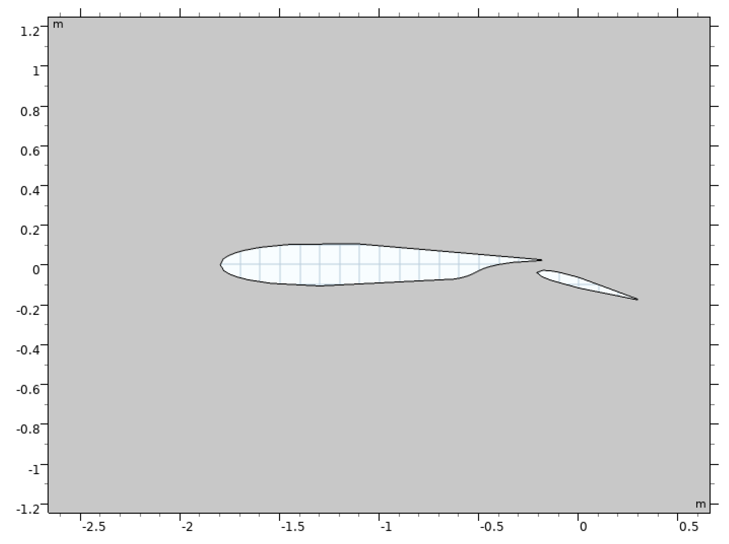
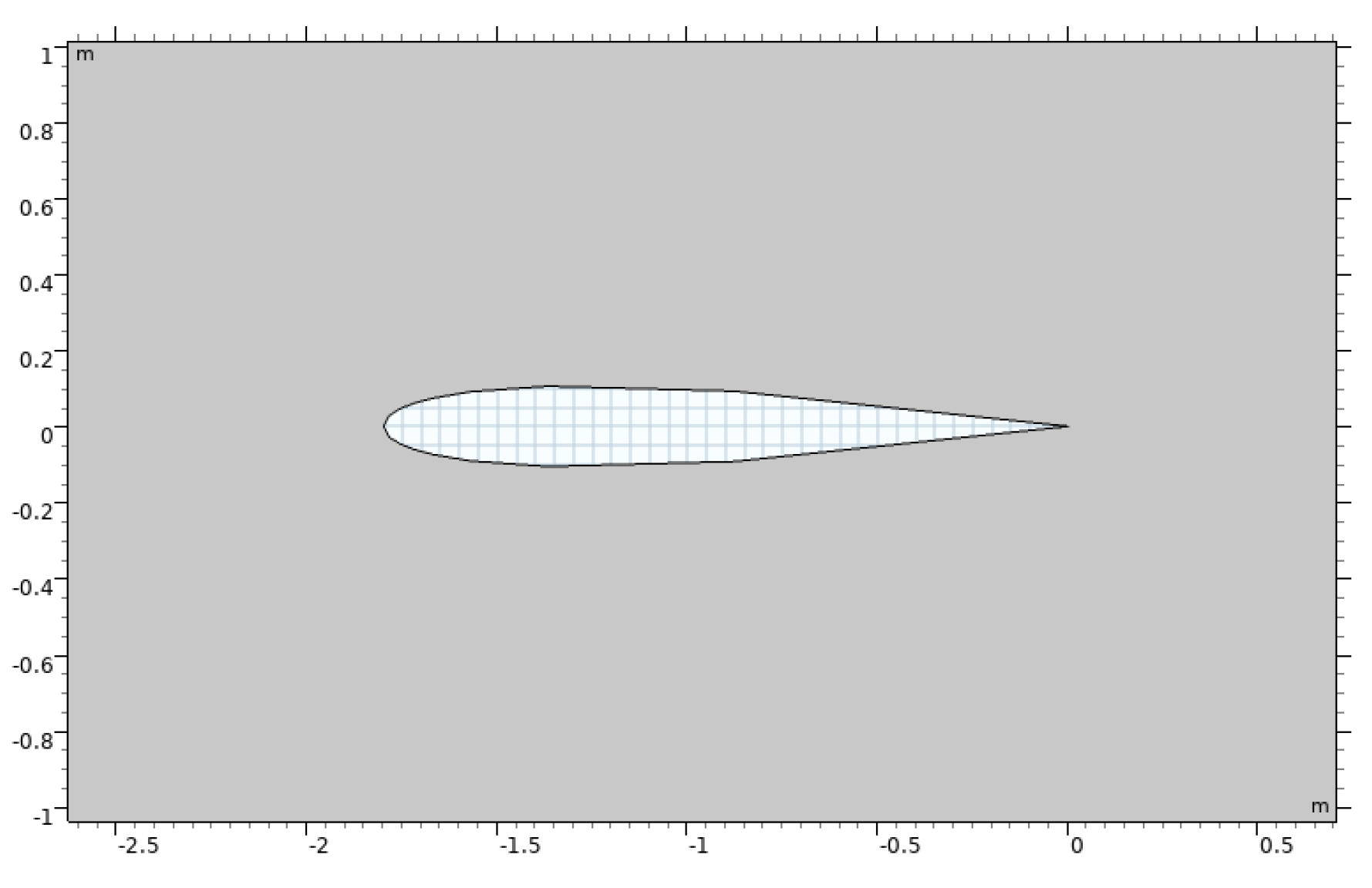
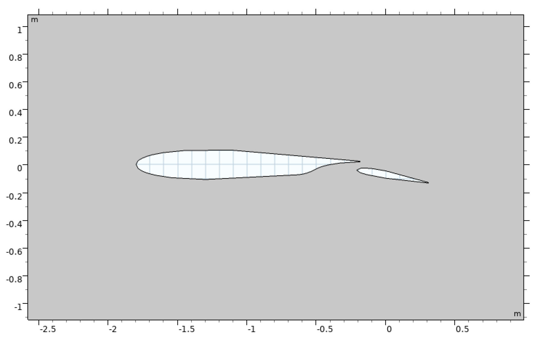
The chord length c is 1.8 m. The resulting airfoil is depicted in Figure 5. Next, the airfoil was modified by adding a slotted flap. Additionally, the rear tips were rounded off. The main wing has a chord length of 1.62 m. The flap has a chord length of 0.53 m. The minimum slot distance between the flap and the main wing is 0.05 m. This airfoil is depicted in Figure 6, where the flap is positioned at 10°. Three flap angles were used in the simulations: 10°, 15°, and 20°. Figure A1 and Figure A2 in Appendix A show the geometry with the flap at 15° and 20°. The 3D model is of the stock NACA 0012, and it has a span of 2 · c = 3.6 m.
The addition of the flap changes the chord length and angle of attack. Additionally, the angle of the flap will also the alter angle of attack and slightly change the chord length. Compared to the chord line of the NACA 0012, the model with the flap has a chord line that is already angled upward with the air coming head on. The chord line is taken as the reference angle of attack, i.e., 0°, from here on out. The air angle adjustments, compared to the stock NACA 0012 and new chord lengths, are listed in Table 1. For example, with the flap at 20°, the relative wind is angled at −6° to obtain an angle of attack of 0°.

2.3.2. Governing Equations and Flow Models

The solver utilizes the conservation of mass and momentum in all flow models which are used. The conservation of mass, also known as the continuity equation, is given by,
ρ t + · ( ρ u ) = 0
where ρ is the density and u is the velocity vector. The conservation of momentum is given by
ρ u t + ρ ( u · ) u = p + · τ ¯ ¯ + F
where p is the static pressure, τ ¯ ¯ is the stress tensor, and F is the volume force vector. The stress tensor can be described by
τ ¯ ¯ = μ ( u + ( u ) T ) 2 3 ( μ · u ) I
where μ is the viscosity and I is the identity matrix. The SST flow model uses two additional transport equations, these are formulated in terms of the turbulent kinetic energy “k” and the specific dissipation rate ω ,
ρ k t + ρ u · k = P ρ β 0 * k ω + · ( ( μ + σ k μ T ) k )
ρ ω t + ρ u · ω = ρ γ μ T P ρ β ω 2 + · ( ( μ + σ ω μ T ) ω ) + 2 ( 1 f v 1 ) ρ σ ω 2 ω ω · k
A full description of the SST model can be found in [33]. COMSOL uses a pseudo time-stepping method based on an adaptive feedback CFL controller. The controller is a multiplicative PID controller given by
C F L n + 1 = e n 1 e n k p t o l e n k i e n 1 / e n e n 2 / e n 1 k d C F L n
where k p , k i , and k d are the controller parameters, e n is the nonlinear error estimate for step n, and t o l is the target error estimate. A lower limit of C F L 1 is used and convergence is not accepted until C F L n C F L = 10 4 , where C F L = 10 4 is the steady-state CFL number.

2.3.3. Boundary Conditions

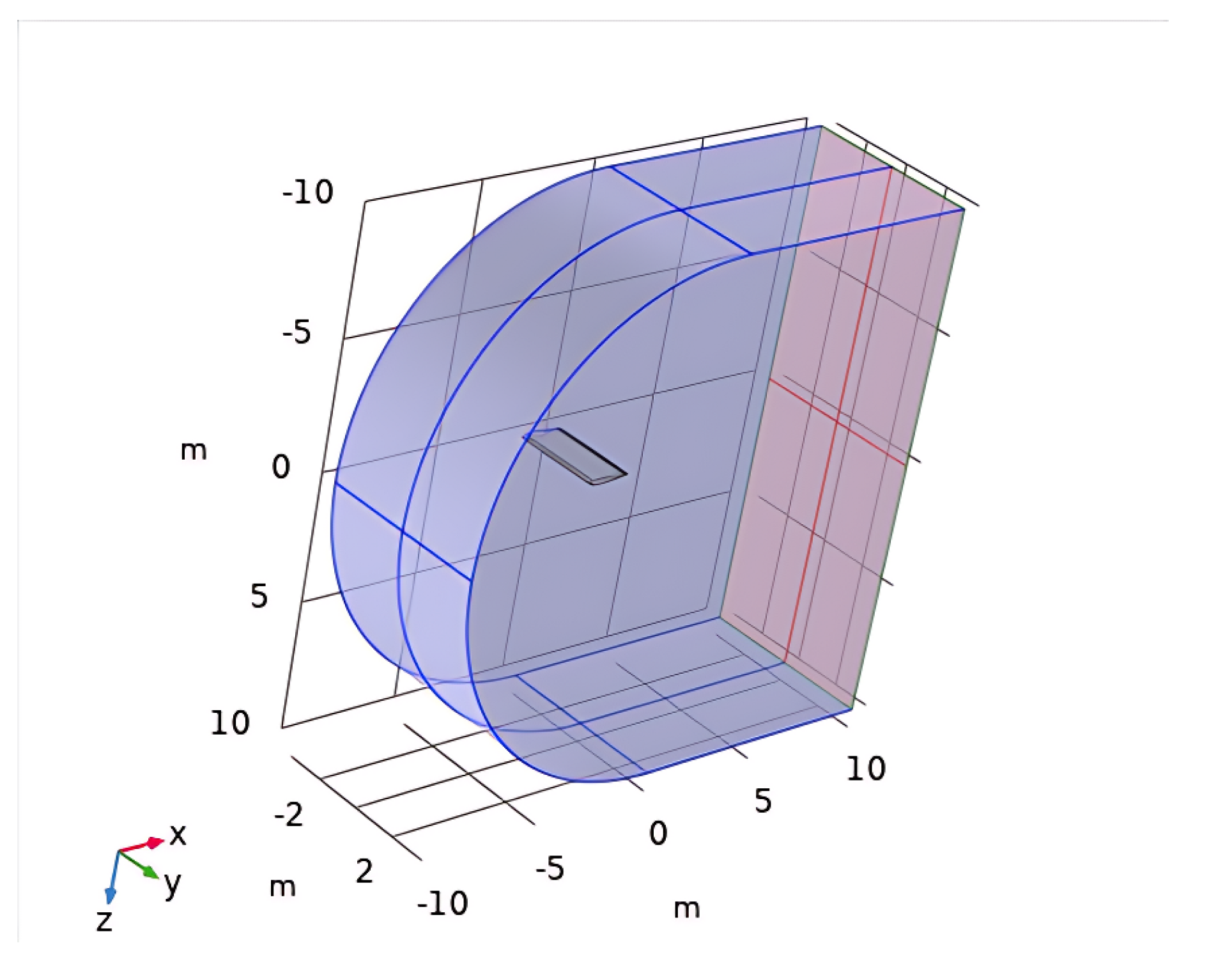
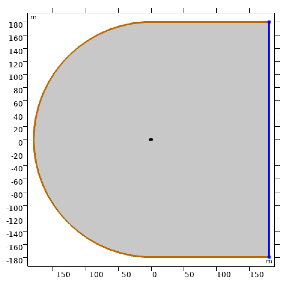
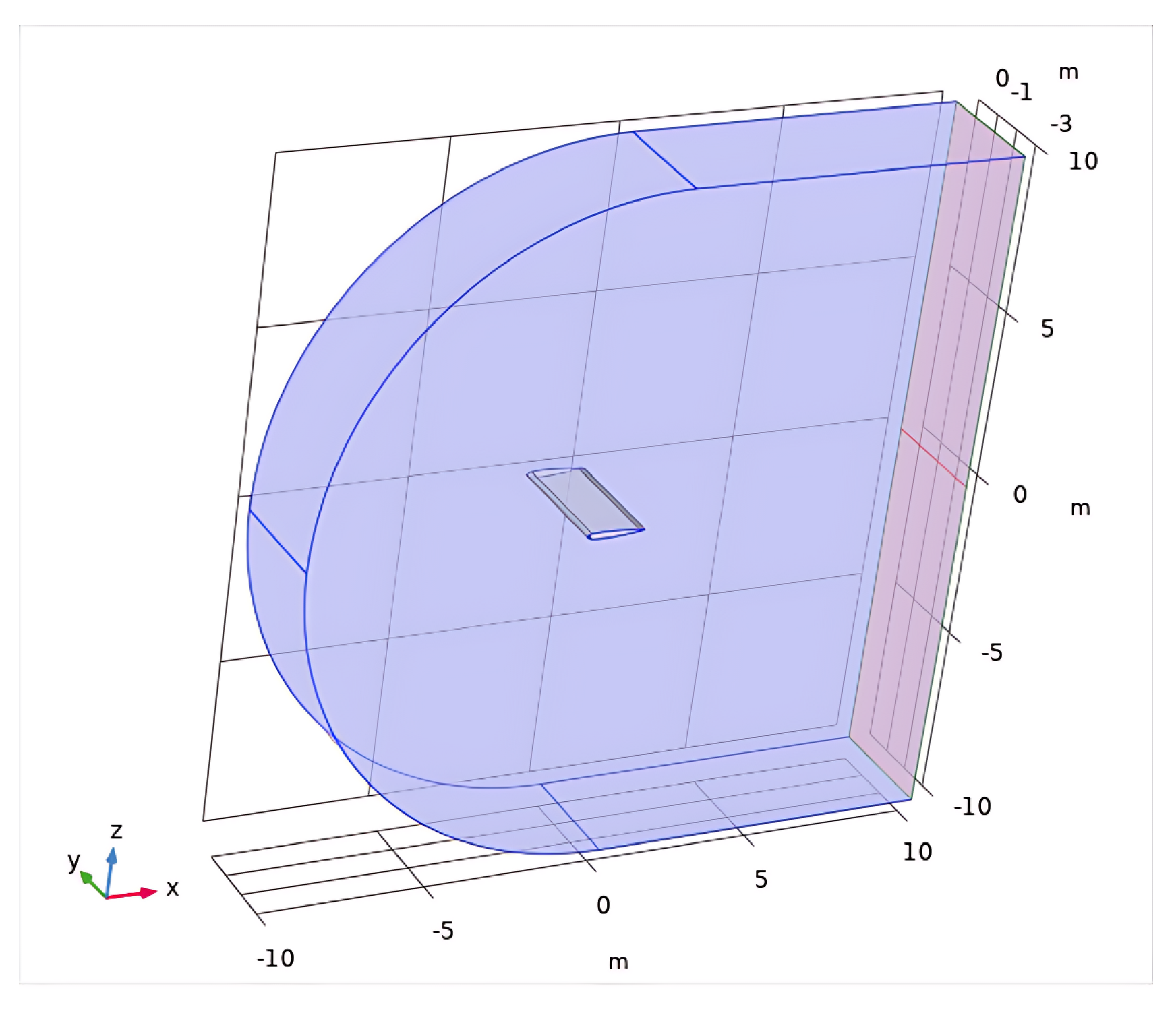
For all 2D models, the reference domain length is L = 180 m. The full domain is depicted in Figure 7; the air flows from left to right, with the inlet depicted in brown and the outlet in blue. This domain shape was selected as it is a commonly used shape in CFD simulations of NACA 0012 airfoils, where a large domain is used to minimize the effect of the boundary conditions [36,37,38,39]. Figure 8 depicts the 3D model domain. Here, the wing spans the entire domain, as such there is no wingtip. The reference length of the domain is reduced to 10 m in order to reduce the computational time and increase the mesh density. The y axis has a length of 2 · c = 3.6 m and is equal to the span of the wing. The blue planes are inlets and the red y z plane in the back is the outlet. The second 3D model has a domain which extends beyond the wing on one side. In turn, this model has a wingtip instead of the wing spanning the entire domain; this model is called “with wingtip”. The domain extends 2 · c = 3.6 m beyond the wingtip in the +y direction, and Figure A3 in Appendix A depicts this domain. The airfoil geometry is assigned the no-slip condition. The parameters used in the simulations are listed in Table 2. The free stream velocity is 50, 75, or 100 m/s for the 2D models and 50 m/s for the 3D model. These values were chosen because the type of airplanes that use the NACA 0012 and similar wings are typically single-engine propeller airplanes, and these are typical speeds used by these types of planes. At higher velocities, the flow will approach Mach numbers of 1 or higher and shockwaves should be visible; however, these speeds are not achieved in practice by airplanes using the NACA 0012. Moreover, a flow model is not suitable for this flow regime. The free-stream turbulent kinetic energy is calculated by
k = 0.1 μ U ρ L
and the free-stream specific dissipation rate by
ω = 10 U L
The free-stream turbulent kinetic energy and specific dissipation rate are used as boundary conditions for the inlet and outlet. The inlet velocity in the x-direction is calculated by
U , x = U cos α π 180
and in the y-direction by
U , y = U sin α π 180
where U is the free stream velocity and α is the angle of attack. α is increased in an auxiliary sweep to model an increasing angle of attack, where the converged results are used for the next step. The outlet is set to have a normal stress of zero N/m 2 . A simple potential flow model is solved for the first angle of attack and used for the initial values of the field for the first step in the auxiliary sweep.

2.3.4. Meshes

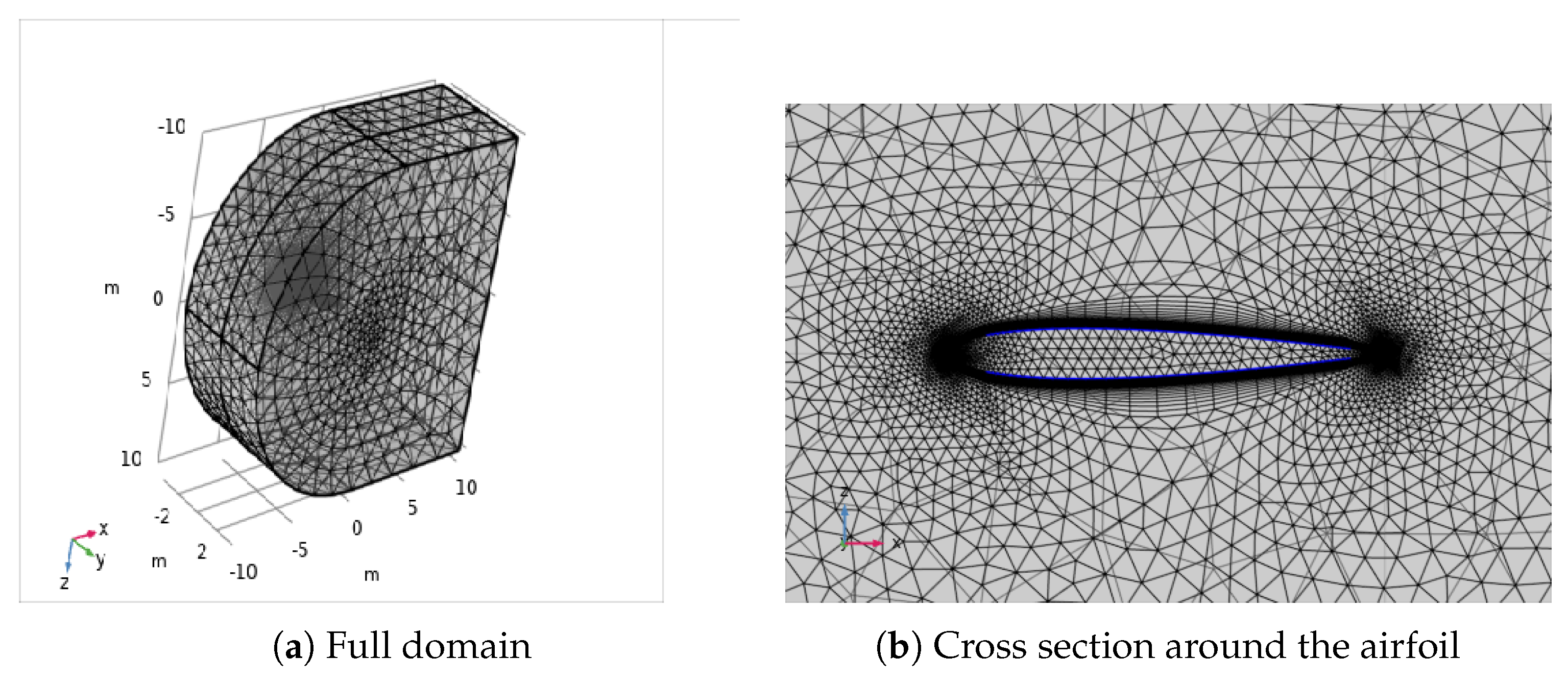
The first meshes were fully generated by COMSOL based on the type of physics included in the model; the only setting changed was the element size setting. The element size setting was varied from extremely coarse to extremely fine. Table 3 lists the specifications of all the COMSOL-generated meshes that were able to converge. These meshes showed poor results compared to experimental results; additionally, finer meshes were unable to converge. Therefore, a reference user-controlled mesh was made. A mapped mesh was used close to the airfoil, and further out, an unstructured triangular mesh was used. This mesh is illustrated in Figure 9, with a close-up around the airfoil in Figure 9b. To make the reference mesh, the outline of the airfoil was enlarged, forming a domain around the airfoil. This domain was split into different sections, allowing more precise control of the element distribution in each section. In each of the split domains, a structured mesh was used with an exponential distribution normal to the airfoil surface, creating thin elements close to the airfoil surface. The distribution of each split domain along the surface was set to have a higher density at the leading and trailing edge of the airfoil, with a lower density in the middle part. This mesh shows good agreement with experimental lift coefficient data. A similar meshing strategy was employed for the modified airfoil, shown in Figure 10, and a close-up around the airfoil is depicted in Figure 10b. The 3D model uses a mix of mapped and unstructured meshes on the airfoil surface. Figure 11b depicts a cross-section of the mesh, and the full mesh is shown in Figure 11a. Table 4 lists the specifications of all the user generated meshes.
The number of mesh boundary layers around the modified airfoil was altered and evaluated with respect to the C L / C D ratio. This was executed with an airspeed of 50 m/s and a flap angle of 10°. The results for four different angles of attack are displayed in Figure 12. An increase from 50 to 75 layers shows a significantly different C L / C D ratio. Additional layers show little change, especially at higher angles of attack. It was decided to use 100 layers to assure accuracy. This also indicates why the COMSOL-generated meshes performed poorly; they employ a significantly lower number of boundary layers and elements.

3. Results and Discussion

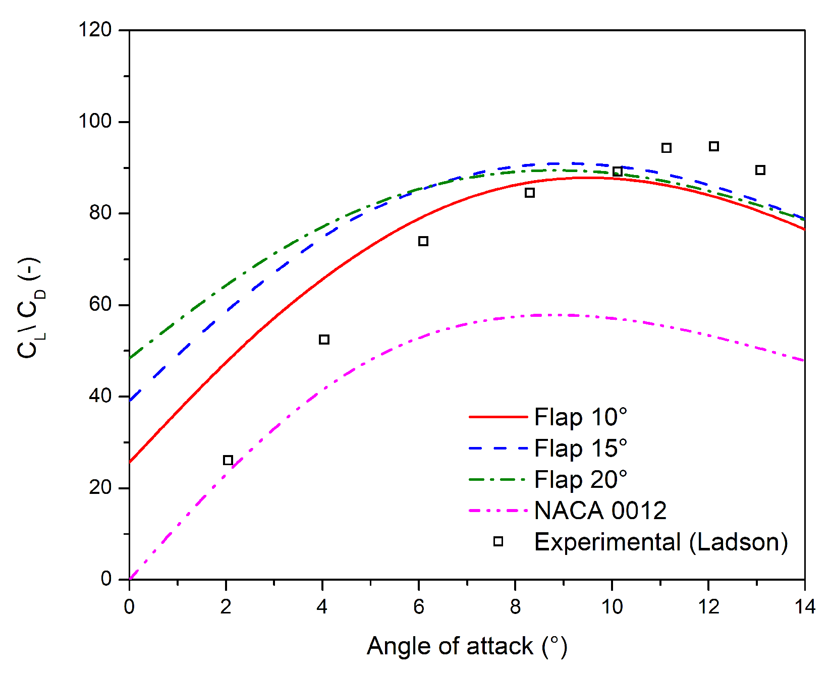
The full results are presented in Appendix B. Of the NACA 0012 simulations using the physics-controlled meshes, only the physics-controlled “extra coarse” and “coarser” meshes converged. The lift coefficients are depicted in Figure 13 alongside the reference user-controlled mesh and experimental data. The reference mesh matches the experimental data closely, showing good agreement overall. The physics-controlled meshes show a similar trend of an increasing lift coefficient with an increasing angle of attack; however, they significantly underestimate the amount of lift. Considering the mesh specifications reported in Table 3 and Table 4, the poor results of the automated meshes can be attributed to the low amount of elements and boundary layers. Consequently, the automated mesh has a low element density throughout, including close to the airfoil itself. In turn, it is unable to accurately capture the boundary layer flow around the airfoil. As a result, the computed lift coefficient is significantly lower than the experimental one. Decreasing the automated element size setting to increase the mesh density does not lead to a solution, as those meshes led to models that were not able to converge.
Overall, these results show how the automated meshes introduce significant deviation from the experimental results. The automated meshes are unsuitable and a user-controlled mesh is required to yield usable results. In turn, user-controlled meshes are used for the investigations into the addition of a slotted flap, the non-isothermal model, and the extension of the stock NACA 0012 airfoil to 3D.

3.1. Modified Airfoil

Figure 14a shows the C L versus the angle of attack for the stock NACA 0012 and the modified airfoil with the three flap angles of 10, 15, and 20. As the modified airfoil is not symmetrical, there is now also lift at α = 0 . The modified airfoils show increased C L compared to the NACA 0012. The NACA 0012 slope begins to decrease at higher α , and as such, the change in lift coefficient between it and the modified airfoils is larger at 14 than 0. These results match the trends found in the literature [20]. The flap increases the C L and the slope gradient remains (mostly) the same. Comparing the different flap angles, a larger angle further increases the C L .
Figure 14b shows the drag coefficients of the same setups mentioned above. Furthermore, NACA 0012 C D data from Ladson [15] are also included. First, we compared the simulated NACA 0012 results to the experimental data. The overall trends match: C D increases with increasing alpha and the slope increases at higher angles. The simulation does significantly overestimate the amount of drag compared to the experimental results. This is due to the flow model assuming the boundary layer is turbulent over the entire length of the airfoil, when in fact, the flow is partially laminar. The laminar flow results in a lower C D , and consequently the C D is overestimated by the flow model [36]. By creating a more fully turbulent boundary layer across the airfoil surface in experiments, for example, by roughening the surface, the results between simulation and experimental would be closer. For example, the simulated results show better agreement with the experimental results from Gregory and O’Reilly when the surface is more roughened [3]. Next, we compared the NACA 0012 to the modified airfoil. The introduction of the flap results in an increase in c D . Compared to the literature, while the high lift device is different, a similar result is observed [20]. In Figure 14b, the NACA 0012 has a higher C D at higher angles of attack than the modified airfoils, this is due to the difference reference angles. If the relative wind was used as α = 0 , the C D of the modified airfoil would be higher for all angles. Additionally, a larger flap angle increases the C D . These results confirm the hypothesis that the modified airfoil would have an increased C L and C D compared to the NACA 0012. These results show how a movable flap can be used to adapt to situations where either the lift or drag coefficient might be more important. The performance can be further improved by adding additional high lift devices, for example, a slat or multiple slotted flaps. The change in performance resulting from the addition of slotted flaps and slats is caused by multiple effects: the slat effect, the circulation effect, the dumping effect, off-the-surface pressure recovery, and the fresh boundary layer effect. A full explanation of all these effects is beyond the scope of this work and can be found in [40].
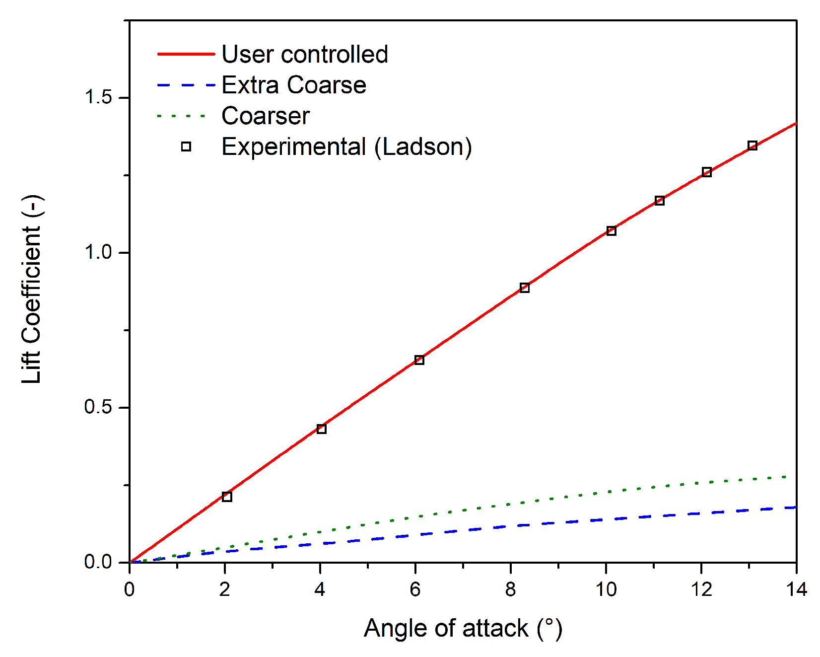
Figure 15 displays the C L / C D ratios. There is a large difference between the NACA 0012 simulation and the Ladson data due to the C D . The profile is similar for all setups, showing a parabolic profile. The reason for this profile shape is that the C D increases exponentially, whereas C L increases linearly. The flap significantly improves the C L / C D ratio compared to the stock NACA 0012 for all angles of attack; additionally, the C L / C D ratio is further improved with larger flap angles.
Overall, the modified airfoil shows significant improvements in C L and C L / C D , and a substantial increase in C D . These results show how a movable flap can be used to adapt to the different stages of flight. For example, the increase in C D is detrimental during cruise flight, but during this stage not much lift is required, and thus the flap can be retracted to a low angle. Conversely, during take off, a lot off lift is desired and the increased drag is an acceptable trade-off; during this stage the flap would be fully extended.
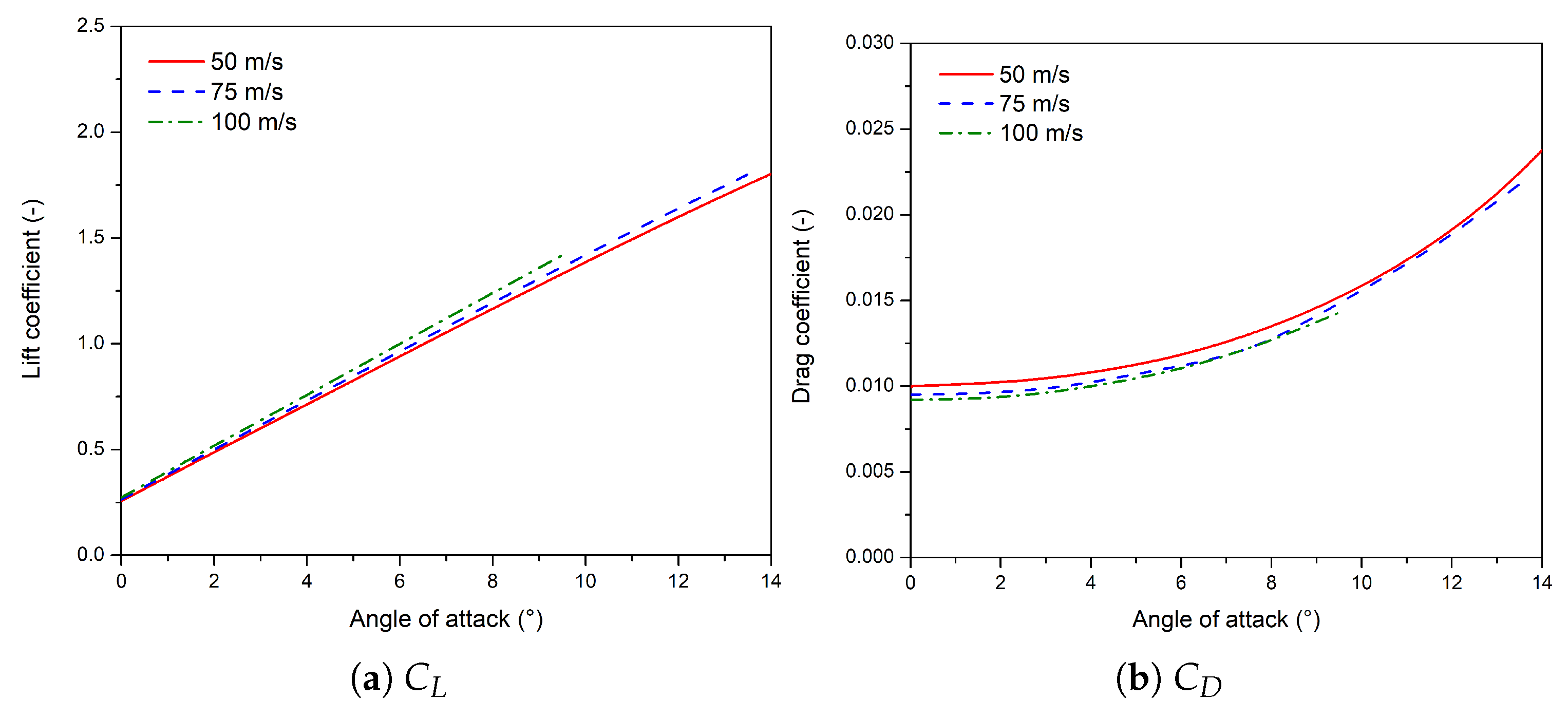
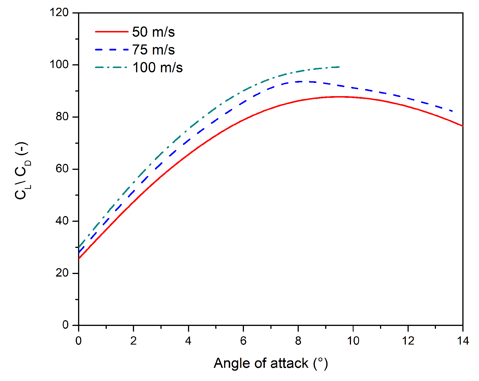
Figure 16a displays the C L for three different free stream velocities: 50, 75, and 100 m/s. The flap is positioned at 10°. There is a very small increase in C L at higher velocities. Figure 16b depicts a small decrease in C D , as was expected from the literature and previous papers [5,20]. With the improvements in C L and C D , their ratio also improves, as depicted in Figure 17.
The simulated results match the expectations from airfoil theory well, showing how numerical simulations can be effectively utilized in the development and optimization of airfoil geometry and flap operation.

3.2. Non-Isothermal Flow

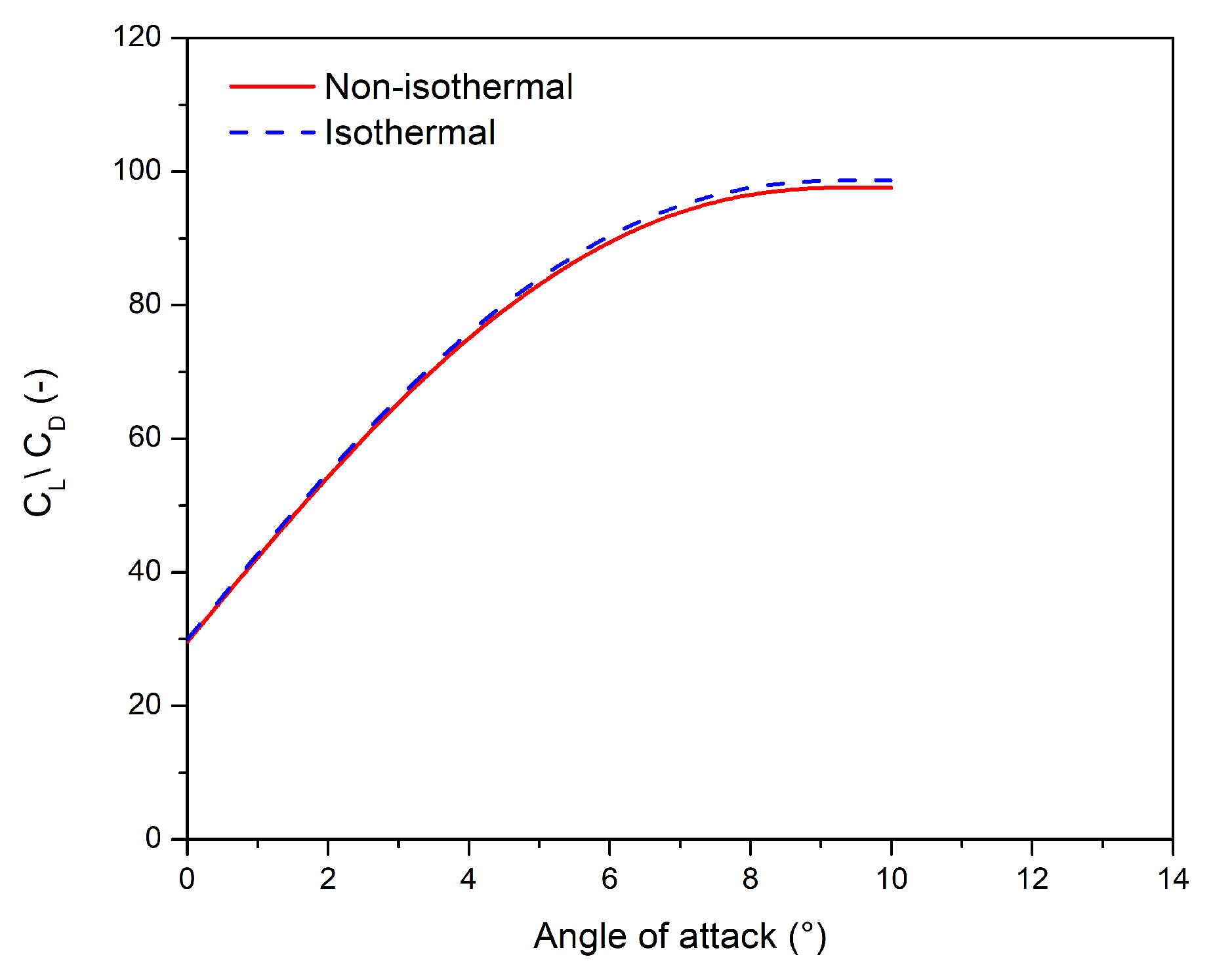
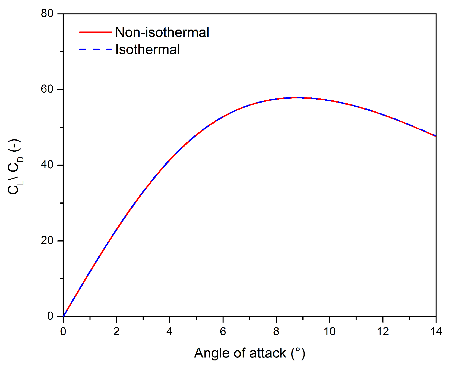
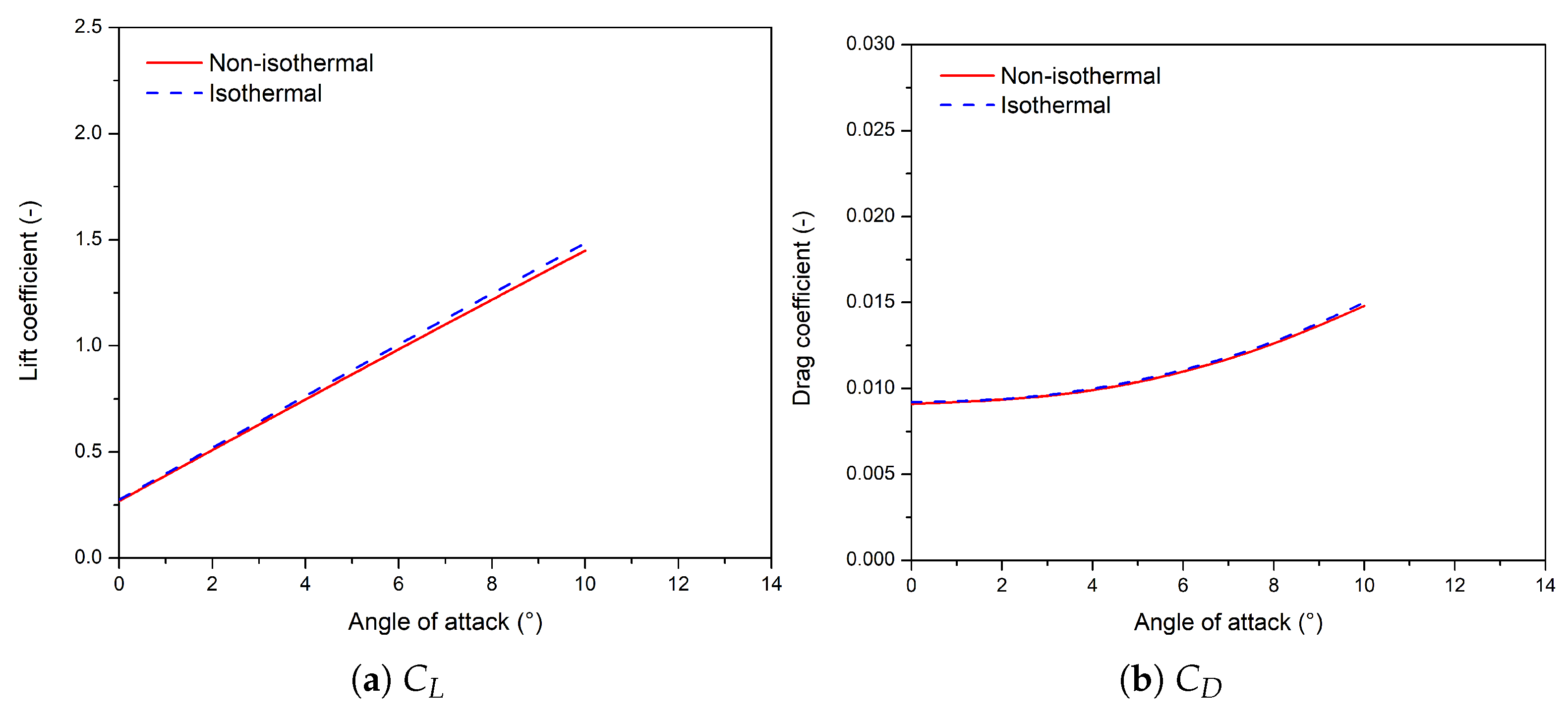
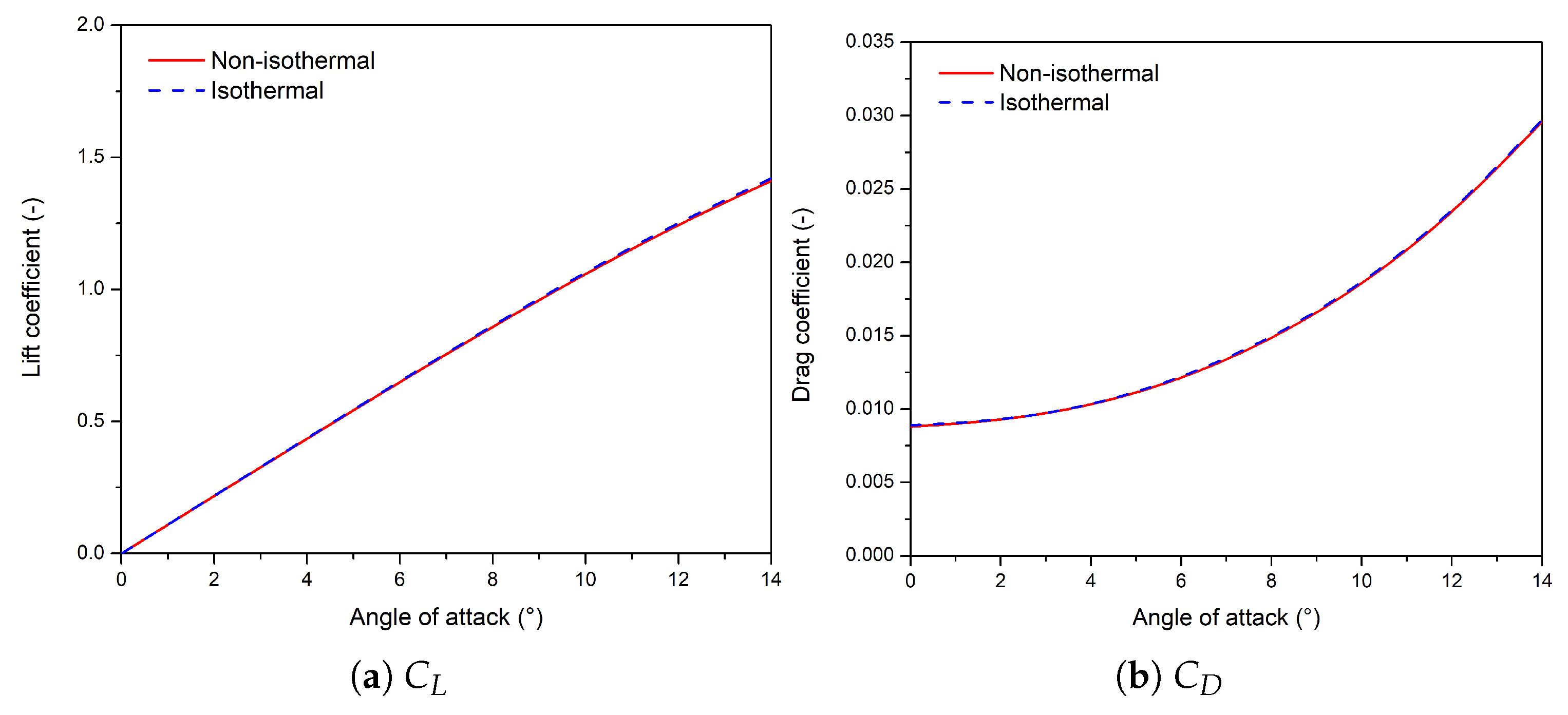
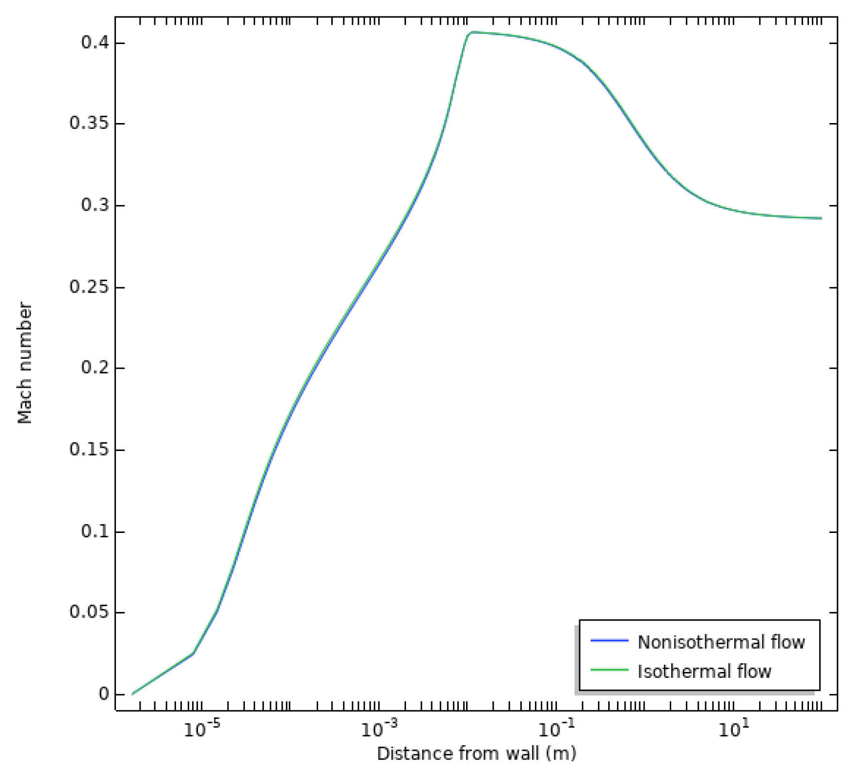
Looking at Figure 18, which compares the isothermal to the non-isothermal simulation of the modified airfoil, there is little difference in C L , C D , and consequently their ratio. A similar result is observed in Figure 19, showing the isothermal versus non-isothermal results for the NACA 0012. Here, the performance is also identical. The Mach number of the flow is largely below 0.3; as such, the flow can be regarded as incompressible and the effect of temperature is small. Based on these results, the use of an isothermal flow model is valid. This is not surprising, as the non-isothermal NACA 0012 simulation already showed good agreement with the experimental C L results.

Wall Profiles

Figure 20 displays the dimensionless velocity profile of the modified airfoil. This profile shows good agreement with the “law of the wall” profile in Figure 4.
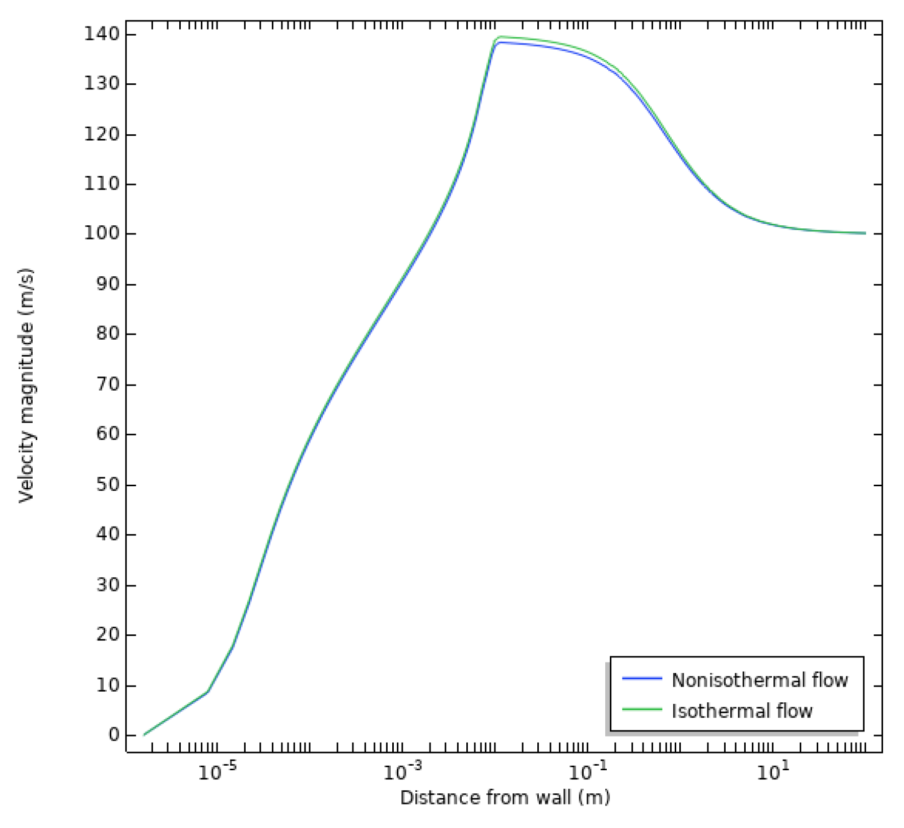
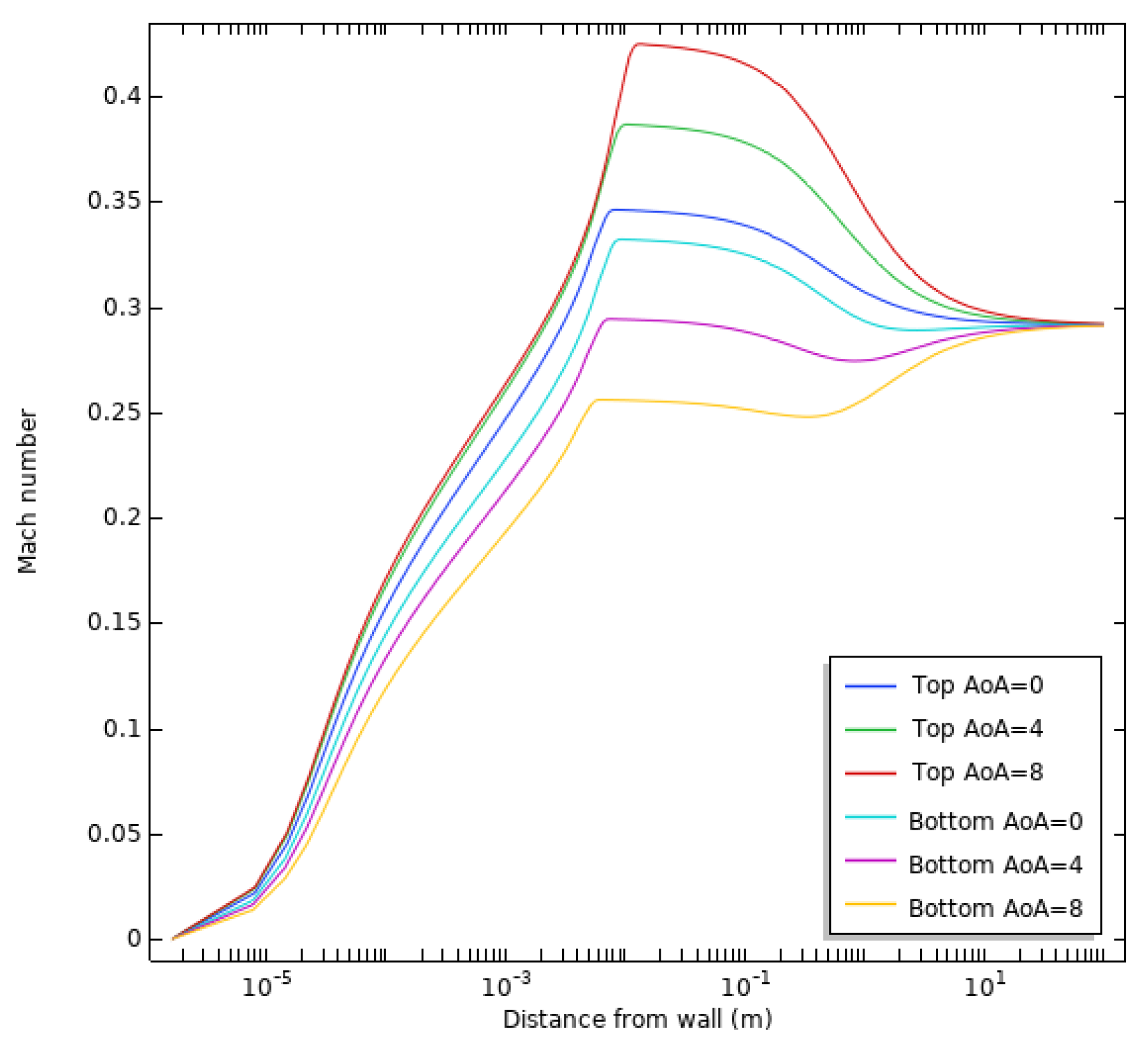
Figure 21, Figure 22, Figure 23 and Figure 24 depict various profiles originating from the modified airfoil wall. These profiles are perpendicular to the thickest point at the top of airfoil and extend 100 m vertically. The angle of attack is 6°. The profile reaches its peak around 0.01 m, after which the velocity normalizes to the free-stream velocity. As the line is stemming from the top of the airfoil, the velocity reaches higher levels than the free stream velocity. There is a very small difference in velocity between the non-isothermal and isothermal model, best seen at the top of the peak. Figure 23 displays a largely similar profile. The difference between the two models with regard to the Mach number is even smaller. Figure 22 depicts the temperature profile; for the isothermal model it is naturally flat. The non-isothermal model shows a profile that is similar to those seen in Figure 21 and Figure 23 but inverted. Figure 24 illustrates the temperature profile but inverted. The temperature peaks at the same distance from the wall as the velocity, and beyond the peak it normalizes to the free-stream temperature in a similar manner. Figure 25 shows the Mach number profiles perpendicular to the thickest point at the top and the bottom of the airfoil. Three different angles of attack are shown. At α = 0 °, the top and bottom profile are close to each other. As the angle increases, the Mach number increases at the top, while it decreases at the bottom. The profile shape for the boundary layer remains the same. Beyond the boundary layer, the profile normalizes to the free-stream Mach number.

3.3. 3D Model

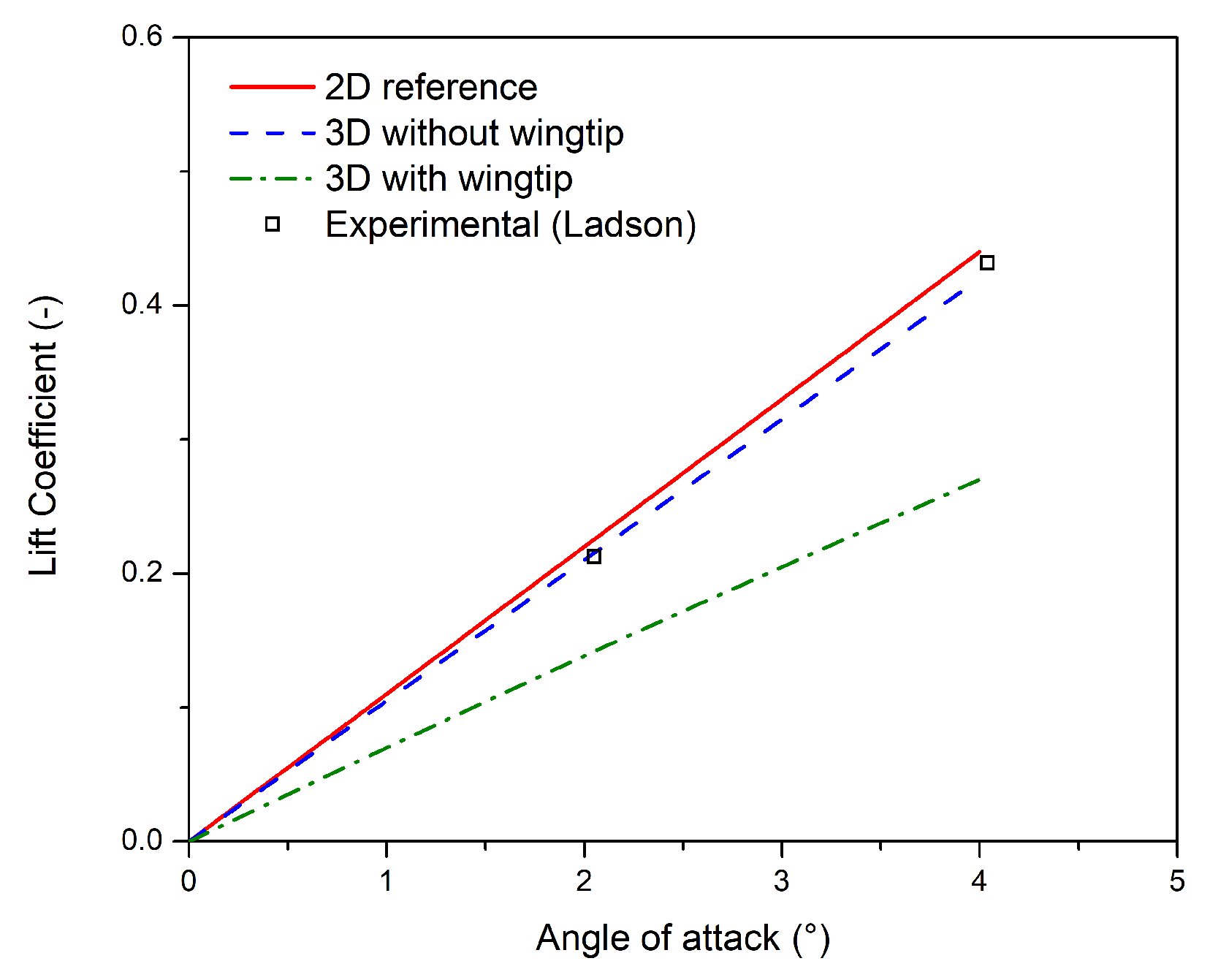
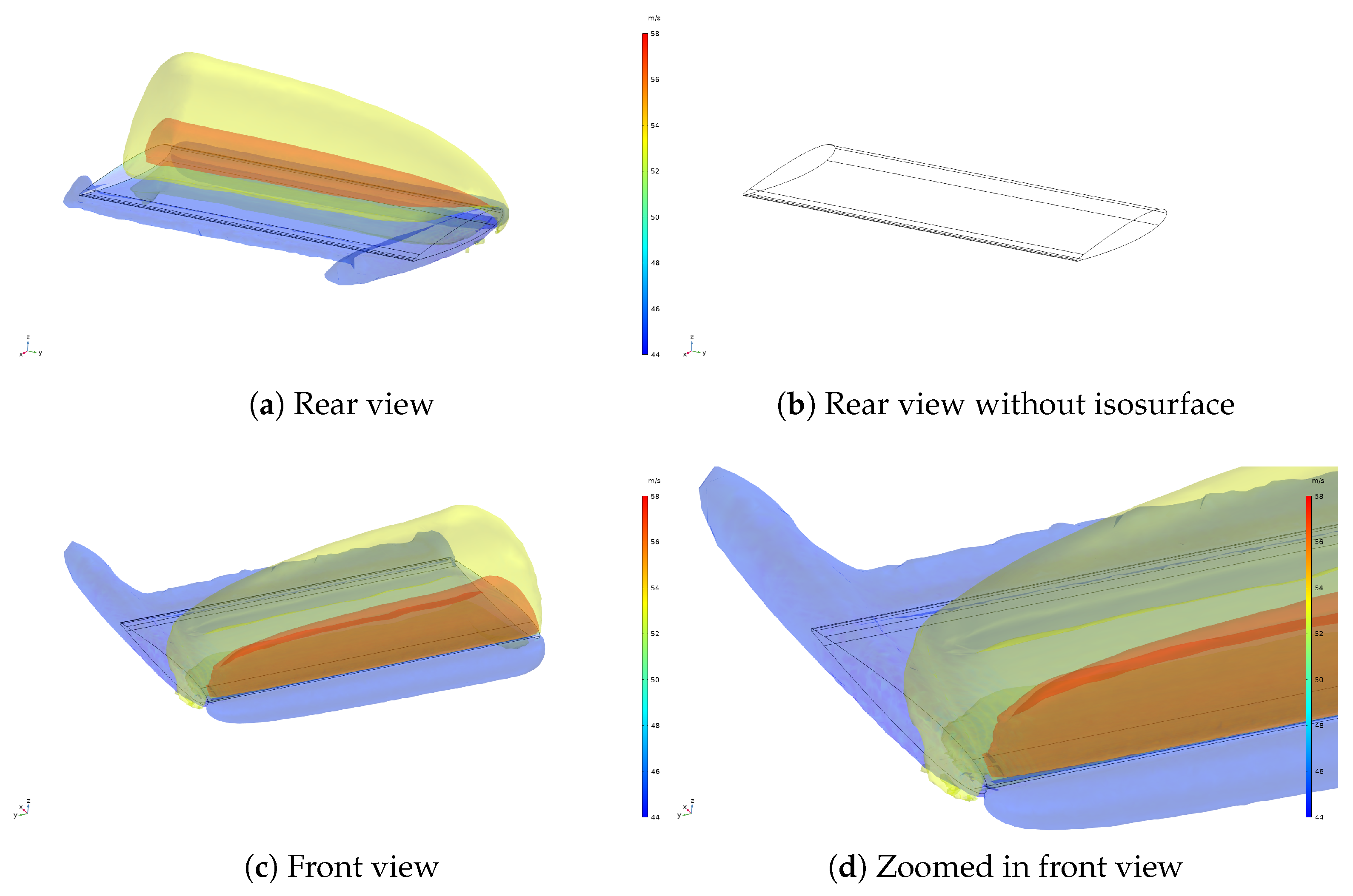
Figure 26 displays the C L of the 3D models compared to the reference 2D model. The 3D model without a wingtip shows good agreement with the experimental data and the 2D model. It is similar as the wing spans the entire domain. The model with a wingtip shows a significantly lower C L , as was predicted from wing theory. Figure 27a illustrates the velocity magnitude isosurface of the NACA 0012 with a wingtip, where the air is flowing in the +x direction. The same view without the isosurface is depicted in Figure 27b to show the position of the wing. At the right bottom of the image is the side of the airfoil with the wingtip. As can be seen, the wingtip has a substantially different profile compared to the side ending in a boundary. The velocity magnitude decreases towards the wingtip. Figure 27c shows the velocity magnitude isosurface viewed from the front of the wing and Figure 27d shows the front zoomed in on the wingtip. Here, it can be well seen how a trail develops behind the wingtip.
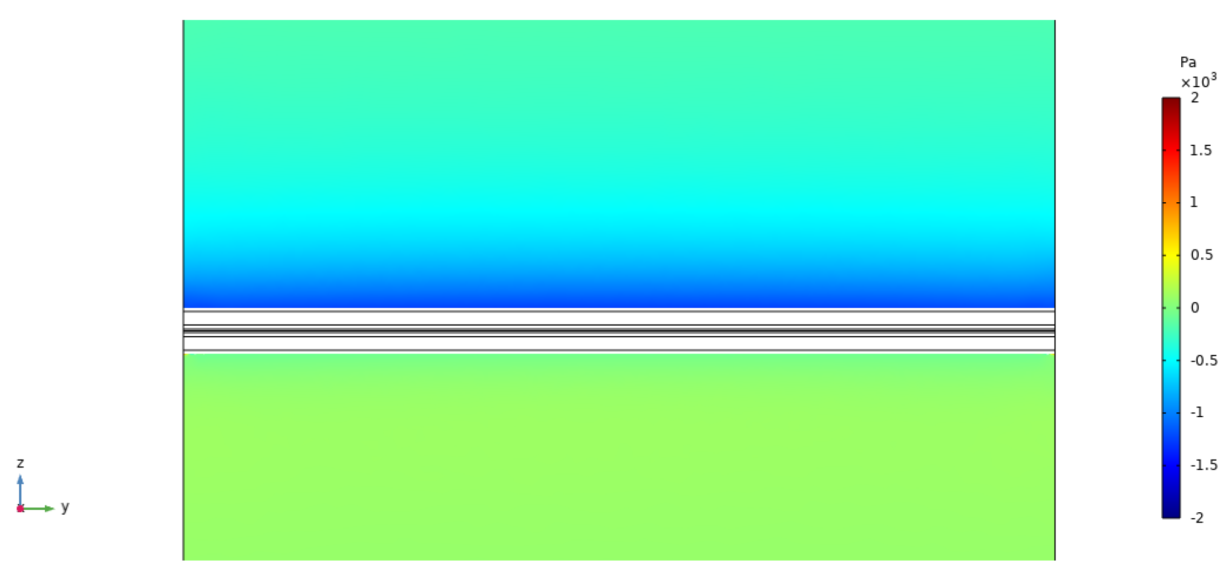
The difference in lift can be further explained by looking at the dynamic pressure profile around the airfoil. Figure 28 and Figure 29 depict slices at two different positions along the span of the wing. First looking at the slices in the middle of the wing in Figure 28a and Figure 29a, the pressure delta between the top and the bottom of the airfoil is lower with a wingtip. Next looking at Figure 28b and Figure 29b, the wingtip has a significantly lower pressure delta. This pressure difference is generating lift, consequently the C L is lower for the model with wingtip.
Figure 30 depicts a yz plane pressure slice, it is positioned 0.15 chord lengths along the wing from the leading edge. On the left, the wing ends at the boundary of the domain, and on the right is the wingtip. The pressure on top increases towards the wingtip, and does so more rapidly close to the wingtip. The air can flow around the wingtip from the high pressure region under the wing to the low pressure region on top. This flow around the wingtip is what creates wingtip vortices. As the fully bounded wing does not allow flow around the wing, it does not exhibit these vortices. Figure 31 displays the yz slice for the model without a wingtip. The air is unable to flow around the wingtip, and as a result, the pressure is constant along the y-axis across the wing.

4. Conclusions

Two- and three-dimensional models of an NACA 0012 were studied in COMSOL under different regimes and analyzing the different physics involved.
  • A first numerical conclusion of this study is that the COMSOL physics-controlled meshing settings are not suitable for this airfoil simulation as they are either unable to converge or give results that do not match those of experiments. User-controlled meshes are required to yield good results.
  • The SST turbulence flow model with a user-controlled mesh shows good agreement with experimental C L results. The C D results need to be considered carefully when trying to apply it to real life wings, as the flow model assumes turbulent flow across the entire airfoil. The degree to which this assumption is valid will depend on the wing roughness. The modified airfoil has increased C L and C L / C D values compared to the stock NACA 0012. Increasing the flap angles further increases C L and C D . The free stream velocity has a minor impact, with a very slightly higher C L and slightly higher C D at higher velocities. Overall, the simulated results correspond well to what is expected from theory and real-life experiments.
  • No significant difference was found in C L or C D between the isothermal and non-isothermal models. In turn, the use of a non-isothermal model is not required for good results in these simulations.
  • The 3D model shows some interesting avenues for future research, but the current results are limited and more verifications are necessary.
For instance, a large eddy simulation (LES) model could be evaluated, especially at higher angles of attack near or at stalling. Different high lift devices could be used to modify the NACA 0012 and compare their performance, for example, a slat at the front. Combinations of these devices could be made to further optimize the airfoil, for example, an additional flap or a combination of a flap and a slat. The shape of the main body could be altered, for example, by using the NASA supercritical (SC) airfoils used in commercial jets. The span could be increased, and this would be especially interesting for the model with a wingtip. Similar modifications which have already been made or suggested for the 2D model could be made for the 3D model.

Author Contributions

Methodology; software; validation; formal analysis; investigation; writing—original draft preparation, B.S. Project administration; conceptualization; resources; writing—review and editing; visualization; supervision, P.D. All authors have read and agreed to the published version of the manuscript.

Funding

This research received no external funding.

Institutional Review Board Statement

Not applicable.

Informed Consent Statement

Not applicable.

Data Availability Statement

Not applicable.

Acknowledgments

B.S. thanks the University of Groningen for providing the COMSOL Multiphysics software. P.D. thanks to Aleksandra Piekorz for her valuable comments about this paper.

Conflicts of Interest

The authors declare no conflict of interest.

Abbreviations

The following abbreviations are used in this manuscript:
CFDComputational Fluid Dynamics
LESLarge Eddy Simulation
NACANational Advisory Committee for Aeronautics
RANSReynolds-Averaged Navier–Stokes
SASpalart–Allmaras
SSTShear-Stress Transport
Nomenclature
AArea (m 2 )
cSpeed of sound (m/s)
C D Drag coefficient (-)
C L Lift coefficient (-)
F D Drag force (N)
F L Lift force (N)
kSpecific heat ratio (-)
pPressure (Pa)
R p Particular gas constant (J/kg · K)
TTemperature (K)
[ u , v , w ] Fluid velocity field (m/s)
Greek Letters
α Angle of attack ()
ρ Fluid density (kg/m 3 )
μ Phase viscosity (mPa · s)

Appendix A. Figures

Figure A1. Modified airfoil geometry with the flap at 15°.
Applsci 13 07890 g0a1
Figure A2. Modified airfoil geometry with the flap at 20°.
Applsci 13 07890 g0a2
Figure A3. Geometry of 3D NACA 0012 with a wingtip on one side. Blue planes are inlets, red planes are outlets.
Applsci 13 07890 g0a3
Figure A4. C L / C D of isothermal and non-isothermal flow for the modified airfoil, with the flap positioned at 10° and an airspeed of 100 m/s.
Applsci 13 07890 g0a4
Figure A5. C L / C D isothermal and non-isothermal flow for an NACA 0012 airfoil with an airspeed of 50 m/s.
Applsci 13 07890 g0a5

Appendix B. CL, CD, and CL/CD Date

Table A1. CL of NACA 0012, SST turbulent flow model with physics-controlled mesh.
AlphaExtra CoarseCoarser
00.000.00
20.040.05
40.060.10
60.090.15
80.120.19
100.140.23
120.160.26
140.180.28
Number of elements17422688
Table A2. CL of modified airfoil.
Flap 10°Flap 15°Flap 20°
Alpha50 m/s75 m/s100 m/sAlpha50 m/s75 m/s100 m/sAlpha50 m/s75 m/s100 m/s
00.2570.2650.2740.00.4120.4250.4420.00.5570.5760.601
20.4890.5020.5202.00.6430.6620.6872.00.7840.8090.842
3.60.6680.6850.7104.00.8720.8960.9294.01.0101.0411.082
5.60.8960.9190.9524.80.9610.9881.0256.01.2331.2691.320
7.61.1221.1491.1936.81.1861.2191.2658.01.4511.4941.555
9.61.3431.3761.4318.81.4071.4461.50210.01.6661.7151.786
11.61.5591.598 10.81.6231.669 12.01.8731.930
13.61.7661.811 12.81.8311.884 14.02.0722.136
15.61.958 14.82.0272.086 16.02.257
16.62.045 16.82.204 18.02.419
17.62.122 17.82.281 19.02.484
18.82.343 20.02.528
Table A3. CD of modified airfoil.
Flap 10°Flap 15°Flap 20°
Alpha50 m/s75 m/s100 m/sAlpha50 m/s75 m/s100 m/sAlpha50 m/s75 m/s100 m/s
0.00.0100.0090.0090.00.0110.0100.0100.00.0120.0110.011
2.00.0100.0100.0092.00.0110.0100.0102.00.0120.0120.011
3.60.0110.0100.0104.00.0120.0110.0114.00.0130.0120.012
5.60.0120.0110.0114.80.0120.0110.0116.00.0140.0140.014
7.60.0130.0120.0126.80.0130.0130.0138.00.0160.0160.015
9.60.0150.0150.0148.80.0150.0150.01510.00.0190.0180.018
11.60.0180.018 10.80.0180.017 12.00.0220.021
13.60.0220.022 12.80.0220.021 14.00.0260.026
15.60.028 14.80.0270.027 16.00.033
16.60.033 16.80.034 18.00.042
17.60.038 17.80.039 19.00.048
18.80.046 20.00.056
Table A4. CL/CD of modified airfoil.
Flap 10°Flap 15°Flap 20°
Alpha50 m/s75 m/s100 m/sAlpha50 m/s75 m/s100 m/sAlpha50 m/s75 m/s100 m/s
025.728.029.90.039.142.645.70.048.452.756.4
248.052.155.72.059.364.268.62.064.970.375.1
3.663.068.572.44.075.181.186.34.077.984.089.2
5.677.783.589.04.880.186.491.96.086.192.497.7
7.686.395.897.86.888.795.2100.88.089.896.0101.0
9.688.791.799.48.891.798.1103.110.089.495.199.2
11.685.888.8 10.889.995.7 12.085.490.5
13.678.882.3 12.884.189.1 14.078.682.7
15.668.8 14.875.378.6 16.069.4
16.662.9 16.864.2 18.058.2
17.656.3 17.858.0 19.051.9
18.851.0 20.045.0
Table A5. Non-isothermal and isothermal of modified airfoil. 100 m/s, flap 10°.
Non-IsothermalIsothermal
AlphaCdClCl/CdCdClCl/Cd
00.00910.26929.60.00920.27529.9
20.00930.50955.00.00930.52055.7
40.00980.74876.10.00990.76476.9
60.01090.98490.70.01101.00791.6
80.01251.21897.80.01261.24798.8
100.01481.44997.60.01501.48498.7
Table A6. NACA 0012, 50 m/s, non-isothermal and isothermal.
Non-IsothermalIsothermal
AlphaCdClCl/CdCdClCl/Cd
00.0090.000.00.0090.000.0
20.0090.2223.80.0090.2223.9
40.0100.4442.70.0100.4442.7
60.0120.6554.00.0120.6554.0
80.0150.8658.30.0150.8658.3
100.0181.0657.70.0181.0757.7
120.0231.2553.70.0231.2553.7
140.0301.4147.60.0301.4247.8
Table A7. CL of 3D models.
Alpha2D Reference3D without Wingtip3D with Wingtip
00.000.000.00
20.220.210.14
40.440.420.27
Table A8. CD of 3D models.
Alpha2D Reference3D without Wingtip3D with Wingtip
00.0090.0240.019
20.0090.0260.020
40.010.0310.026
Table A9. CL/CD of 3D models.
Alpha2D Reference3D without Wingtip3D with Wingtip
00.00.00.0
224.48.36.6
443.813.710.5

References

  1. Hirsch, C. Numerical Computation of Internal and External Flows: Introduction to the Fundamentals of CFD; Butterworth-Heinemann: Oxford, UK, 2007. [Google Scholar]
  2. Ouahabi, M.H.; El Khachine, H.; Benabdelouahab, F. Aerodynamic Analysis of Wind Turbine Blade of NACA 0006 Using a CFD Approach. In Proceedings of the WITS 2020, Fez, Morocco, 14–16 October 2020; Bennani, S., Lakhrissi, Y., Khaissidi, G., Mansouri, A., Khamlichi, Y., Eds.; Springer: Singapore, 2022; pp. 541–552. [Google Scholar]
  3. Gregory, N.; O’Reilly, C.L. Low-Speed Aerodynamic Characteristics of NACA 0012 Aerofoil Section, including the Effects of Upper-Surface Roughness Simulating Hoar Frost; AERADE: Cranfield, UK, 1970. [Google Scholar]
  4. Du, Y.; Gao, Z.; Wang, C.; Huang, J. Experiment and Numerical Simulation of Crossflow Transition on A Large-Swept Supercritical Tapered Thin Wing Based on Surface Roughness. In Processing of the 11th Asian Computational Fluid Dynamics Conference (ACFD11), Dalian, China, 16–20 September 2016. [Google Scholar]
  5. Hasham Ali, M.; Nawazish Mehdi, S.; Naik, M. Comparative analysis of low velocity vertical axis wind turbine NACA blades at different attacking angles in CFD. Mater. Today Proc. 2021, 80, 2091–2100. [Google Scholar] [CrossRef]
  6. Blinov, V.L.; Zubkov, I.S. Influence of the axial compressor blade row defects on the industrial gas turbine performance. J. Phys. Conf. Ser. 2020, 1683, 42–49. [Google Scholar] [CrossRef]
  7. Irfan Sadaq, S.; Nawazish Mehdi, S.; Danish Mehdi, S.; Yasear, S. Analysis of NACA 0020 aerofoil profile rotor blade using CFD approach. Mater. Today Proc. 2022, 64, 147–160. [Google Scholar] [CrossRef]
  8. Yossri, W.; Ben Ayed, S.; Abdelkefi, A. Airfoil type and blade size effects on the aerodynamic performance of small-scale wind turbines: Computational fluid dynamics investigation. Energy 2021, 229, 120739. [Google Scholar] [CrossRef]
  9. Wenzinger, C.J.; Harris, T.A. Wind-Tunnel Investigation of an NACA 23012 Airfoil with Various Arrangements of Slotted Flaps; Technical Report; NASA: Washington, DC, USA, 1939. [Google Scholar]
  10. Todorov, M. Aerodynamic Characteristics of Airfoil with Single Slotted Flap for Light Airplane Wing. In Proceedings of the International Conference of Scientific Paper AFASES 2015, Brasov, Romania, 28–30 May 2015; pp. 509–514. [Google Scholar]
  11. Hussein, E.; Azziz, H.; Rashid, F. Aerodynamic study of slotted flap for NACA 24012 airfoil by dynamic mesh techniques and visualization flow. J. Therm. Eng. 2021, 7, 230–239. [Google Scholar] [CrossRef]
  12. Prabhakar, A. CFD analysis on MAV NACA 2412 Wing in high lift take-off configuration for enhanced lift generation. J. Aeronaut. Aerosp. Eng. 2013, 2, 5. [Google Scholar] [CrossRef] [Green Version]
  13. Saha, N. Gap Size Effect on Low Reynolds Number Wind Tunnel Experiments. Ph.D. Thesis, Virginia Tech, Blacksburg, VA, USA, 1999. [Google Scholar]
  14. Yavuz Hakan Ozdemir, B.B. 2D and 3D Potential Flow Simulations around NACA 0012 with Ground Effect. Res. Sq. 2021, preprint. [Google Scholar]
  15. Ladson, C.L. Effects of Independent Variation of Mach and Reynolds Numbers on the Low-Speed Aerodynamic Characteristics of the NACA 0012 Airfoil Section; NASA: Washington, DC, USA, 1988. [Google Scholar]
  16. Chakraborty, S.; Ghosh, S. A CFD study on the structural parameters of NACA 2412 airfoil based air-wing using different composite materials. Mater. Today Proc. 2022, 60, 894–901. [Google Scholar] [CrossRef]
  17. Çakıroğlu, R.; Erdi Tanurun, H.; Acir, A.; Üçgül, F.; Olkun, S. Optimization of NACA 4412 augmented with a gurney flap by using grey relational analysis. J. Braz. Soc. Mech. Sci. Eng. 2023, 45, 167. [Google Scholar] [CrossRef]
  18. Yusop, F.; Mustafa, S.S.; Awang, M.; Hassan, N.N.M.; Noor, H.M. Comparison of Pressure Distribution of NACA 0012 Between CFD Code and Experimental. CFD Lett. 2022, 14, 35–41. [Google Scholar] [CrossRef]
  19. Loutun, M.J.T.; Didane, D.H.; Batcha, M.F.M.; Abdullah, K.; Ali, M.F.M.; Mohammed, A.N.; Afolabi, L.O. 2D CFD Simulation Study on the Performance of Various NACA Airfoils. CFD Lett. 2021, 13, 38–50. [Google Scholar] [CrossRef]
  20. White, F.M. Fluid Mechanics, 8th ed.; McGraw-Hill Education: New York, NY, USA, 2016; pp. 492–499. [Google Scholar]
  21. Anderson, J.D. Fundamentals of Aerodynamics, 6th ed.; McGraw-Hill Education: New York, NY, USA, 2017; pp. 567–577. [Google Scholar]
  22. Jacobs, E.N.; Pinkerton, R.M.; Ward, K.E. The Characteristics of 78 Related Airfoil Sections from Tests in the Variable-Density Wind Tunnel; NACA: Hampton, VA, USA, 1933. [Google Scholar]
  23. Rao, Y.S.R.; Manohar, M.V.N.S.; Praveen, S.V.V.S. CFD simulation of NACA airfoilsat various angles of attack. IOP Conf. Ser. Mater. Sci. Eng. 2021, 1168, 012011. [Google Scholar] [CrossRef]
  24. Cihan, B. Numerical drag reduction of a ground vehicle by NACA2415 airfoil structured vortex generator and spoiler. Int. J. Automot. Technol. 2019, 20, 943–948. [Google Scholar] [CrossRef]
  25. Rogowski, K.; Królak, G.; Bangga, G. Numerical Study on the Aerodynamic Characteristics of the NACA 0018 Airfoil at Low Reynolds Number for Darrieus Wind Turbines Using the Transition SST Model. Processes 2021, 9, 477. [Google Scholar] [CrossRef]
  26. Michna, J.; Rogowski, K. Numerical Study of the Effect of the Reynolds Number and the Turbulence Intensity on the Performance of the NACA 0018 Airfoil at the Low Reynolds Number Regime. Processes 2022, 10, 1004. [Google Scholar] [CrossRef]
  27. Hussein, E.; El, M. Boundary-Layer Theory of Fluid Flow past a Flat-Plate: Numerical Solution using MATLAB. Int. J. Comput. Appl. 2018, 180, 6–8. [Google Scholar] [CrossRef]
  28. Reggente, M. Statistical Gas Distribution Modelling for Mobile Robot Applications. Ph.D. Thesis, Örebro University, Örebro, Sweden, 2014. [Google Scholar]
  29. Rashid, F.L.; Abd, H.S.; Hussein, E.Q. Numerical study of the air flow over modified NACA 2412 airfoil using CFD. AIP Conf. Proc. 2022, 2415, 020005. [Google Scholar] [CrossRef]
  30. Abobaker, M.; Elfaghi, A.M.; Addeep, S. Numerical Study of Wind-Tunnel Wall Effects on Lift and Drag Characteristics of NACA 0012 Airfoil. CFD Lett. 2020, 12, 72–82. [Google Scholar] [CrossRef]
  31. Benoit, M.; Roger, M.; Bosschaerts, W. Multidisciplinary Optimization of Aircraft Propeller Blades. Ph.D. Thesis, Royal Military Academy, Camberley, UK, 2011. [Google Scholar]
  32. Lyu, P. How Do I Compute Lift and Drag? 2015. Available online: https://www.comsol.com/blogs/how-do-i-compute-lift-and-drag/ (accessed on 15 June 2022).
  33. Menter, F.R. Two-equation eddy-viscosity turbulence models for engineering applications. AIAA J. 1994, 32, 1598–1605. [Google Scholar] [CrossRef] [Green Version]
  34. Menter, F.R.; Kuntz, M.; Langtry, R. Ten years of industrial experience with the SST turbulence model. Turbul. Heat Mass Transf. 2003, 4, 625–632. [Google Scholar]
  35. NASA. Menter Shear Stress Transport Model. 2021. Available online: https://turbmodels.larc.nasa.gov/sst.html (accessed on 1 May 2023).
  36. Douvi, C.E.; Tsavalos, I.A.; Margaris, P.D. Evaluation of the turbulence models for the simulation of the flow over a National Advisory Committee for Aeronautics (NACA) 0012 airfoil. J. Mech. Eng. Res. 2012, 4, 100–111. [Google Scholar]
  37. Fatahian, E.; Lohrasbi Nichkoohi, A.; Salarian, H.; Khaleghinia, J. Effects of the hinge position and suction on flow separation and aerodynamic performance of the NACA 0012 airfoil. J. Braz. Soc. Mech. Sci. Eng. 2020, 42, 86. [Google Scholar] [CrossRef]
  38. Shan, H.; Jiang, L.; Liu, C. Direct numerical simulation of flow separation around a NACA 0012 airfoil. Comput. Fluids 2005, 34, 1096–1114. [Google Scholar] [CrossRef]
  39. Uranai, S.; Fukudome, K.; Mamori, H.; Fukushima, N.; Yamamoto, M. Numerical simulation of the anti-icing performance of electric heaters for icing on the NACA 0012 airfoil. Aerospace 2020, 7, 123. [Google Scholar] [CrossRef]
  40. Smith, A.M. High-lift aerodynamics. J. Aircr. 1975, 12, 501–530. [Google Scholar] [CrossRef] [Green Version]
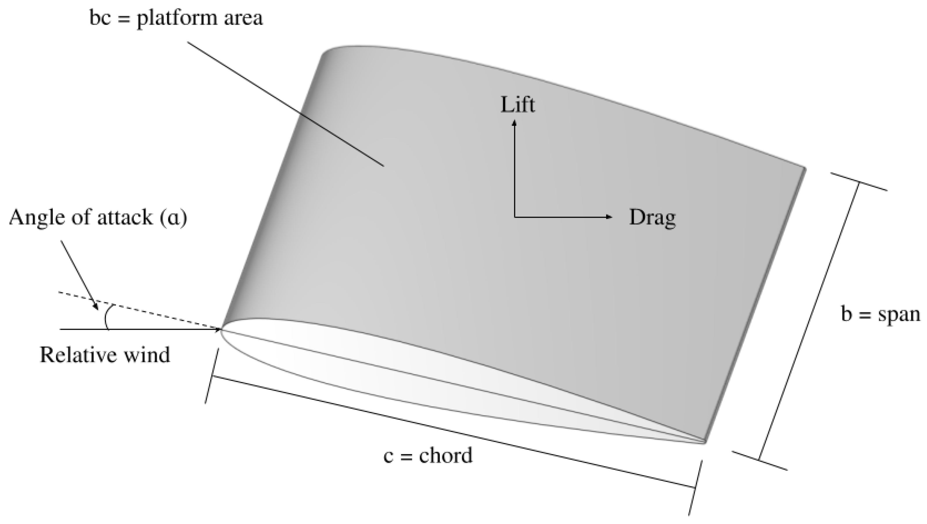
Figure 1. Sketch of a wing with the main parts identified.
Applsci 13 07890 g001
Figure 2. Fluid flow over a flat plate [27].
Applsci 13 07890 g002
Figure 3. Decomposition of the flow variable u into the mean u ¯ and local oscillation u .
Applsci 13 07890 g003
Figure 4. Velocity profile near the wall [31].
Applsci 13 07890 g004
Figure 5. NACA 0012 airfoil geometry.
Applsci 13 07890 g005
Figure 6. Modified airfoil geometry, flap at 10°.
Applsci 13 07890 g006
Figure 7. Boundary conditions of the domain, where the brown boundary is an inlet and the blue boundary is an outlet.
Applsci 13 07890 g007
Figure 8. Boundaries of the 3D model without air beyond the wingtip. The yz plane in the back (red) is the outlet and the other (blue) boundaries are inlets.
Applsci 13 07890 g008
Figure 9. User-controlled mesh of the 2D NACA 0012.
Applsci 13 07890 g009
Figure 10. Mesh of the modified airfoil.
Applsci 13 07890 g010
Figure 11. Mesh of the 3D model with a wingtip.
Applsci 13 07890 g011
Figure 12. C L / C D ratio versus increasing mesh boundary layer count.
Applsci 13 07890 g012
Figure 13. Lift coefficients of physics-controlled automated meshes and the user-controlled mesh compared to experimental data from Ladson.
Applsci 13 07890 g013
Figure 14. NACA 0012 compared to the modified airfoil with the flap positioned at 10°, 15°, and 20° and an airspeed of 50 m/s.
Applsci 13 07890 g014
Figure 15. C L / C D of NACA 0012 compared to the modified airfoil with the flap positioned at 10°, 15°, and 20° and an airspeed of 50 m/s.
Applsci 13 07890 g015
Figure 16. Modified airfoil with the flap positioned at 10°, for airspeeds of 50, 75, and 100 m/s.
Applsci 13 07890 g016
Figure 17. C L / C D of modified airfoil with the flap positioned at 10° for airspeeds of 50, 75, and 100 m/s.
Applsci 13 07890 g017
Figure 18. Isothermal and non-isothermal flow for the modified airfoil, with the flap positioned at 10° and an airspeed of 100 m/s.
Applsci 13 07890 g018
Figure 19. Isothermal and non-isothermal flow for NACA 0012 airfoil with an airspeed of 50 m/s.
Applsci 13 07890 g019
Figure 20. Dimensionless velocity wall profile of the modified airfoil. Air speed 100 m/s, flap angle 10, non-isothermal model.
Applsci 13 07890 g020
Figure 21. Velocity profile.
Applsci 13 07890 g021
Figure 22. Temperature profile.
Applsci 13 07890 g022
Figure 23. Mach number profile.
Applsci 13 07890 g023
Figure 24. Inverted temperature profile.
Applsci 13 07890 g024
Figure 25. Mach number profiles of the modified airfoil with a non-isothermal flow. The cut line starts at the thickest point at the top and bottom of the airfoil, extending vertically for 100 m.
Applsci 13 07890 g025
Figure 26. Lift coefficient of the 3D models.
Applsci 13 07890 g026
Figure 27. Velocity magnitude isosurface of NACA 0012 with a wingtip. The air is flowing in the +x direction.
Applsci 13 07890 g027
Figure 28. Pressure slices of the 3D NACA 0012 without a wingtip (xz plane).
Applsci 13 07890 g028
Figure 29. Pressure slices of the 3D NACA 0012 with a wingtip (xz plane).
Applsci 13 07890 g029
Figure 30. Pressure slice of the 3D NACA with a wingtip. The slice is positioned at 0.15 chord lengths from the leading edge (yz plane).
Applsci 13 07890 g030
Figure 31. Pressure slice of the 3D NACA without a wingtip. The slice is positioned at 0.15 chord lengths from the leading edge (yz plane).
Applsci 13 07890 g031
Table 1. Air angle adjustments and chord lengths.
Flap AngleWind Angle AdjustmentChord Length (m)
No flap0.001.80
10−3.552.11
15−4.782.10
20−6.012.09
Table 2. Model parameters.
SymbolValueDescription
U Variable m/sFree-stream velocity
ρ 1.2043 kg/m3Free-stream density
μ 1.814 ×   10 5 Pa·sFree-stream dynamic viscosity
P101,325 PaFree-stream pressure
T293.13 KFree-stream temperature
C1.8 mChord length
α VariableAngle of attack
Table 3. Meshes generated by COMSOL for the stock NACA 0012.
COMSOL ElementNumber ofAverage ElementNumber of
Size SettingElementsSkewness QualityBoundary Layers
Extra coarse17420.87012
Coarser26880.88112
Table 4. User-controlled meshes.
Airfoil GeometryFlapNumber ofAverage ElementNumber of
AngleElementsSkewness QualityBoundary Layers
2D NACA 0012-52,2400.796100
Modified with flap10105,8000.738100
Modified with flap15105,7520.743100
Modified with flap20105,7550.745100
3D no wingip-665,1310.75025
3D with wingtip-1,169,5790.73540
Disclaimer/Publisher’s Note: The statements, opinions and data contained in all publications are solely those of the individual author(s) and contributor(s) and not of MDPI and/or the editor(s). MDPI and/or the editor(s) disclaim responsibility for any injury to people or property resulting from any ideas, methods, instructions or products referred to in the content.