Hyperspectral Point Cloud Projection for the Semantic Segmentation of Multimodal Hyperspectral and Lidar Data with Point Convolution-Based Deep Fusion Neural Networks

Abstract

The fusion of dissimilar data modalities in neural networks presents a significant challenge, particularly in the case of multimodal hyperspectral and lidar data. Hyperspectral data, typically represented as images with potentially hundreds of bands, provide a wealth of spectral information, while lidar data, commonly represented as point clouds with millions of unordered points in 3D space, offer structural information. The complementary nature of these data types presents a unique challenge due to their fundamentally different representations requiring distinct processing methods. In this work, we introduce an alternative hyperspectral data representation in the form of a hyperspectral point cloud (HSPC), which enables ingestion and exploitation with point cloud processing neural network methods. Additionally, we present a composite fusion-style, point convolution-based neural network architecture for the semantic segmentation of HSPC and lidar point cloud data. We investigate the effects of the proposed HSPC representation for both unimodal and multimodal networks ingesting a variety of hyperspectral and lidar data representations. Finally, we compare the performance of these networks against each other and previous approaches. This study paves the way for innovative approaches to multimodal remote sensing data fusion, unlocking new possibilities for enhanced data analysis and interpretation.

1. Introduction

Hyperspectral and lidar remote sensing technologies are powerful tools for characterizing the Earth’s surface and features in great detail. While hyperspectral sensors offer a high spectral resolution for identifying and mapping the chemical and physical properties of materials, lidar sensors provide high spatial resolution for measuring the height and structure of vegetation and terrain [1]. Fusing these two data sources can provide a more comprehensive understanding of various phenomena and their dynamics. This leads to better-informed decision-making for a wide range of applications such as land use land cover [2], ecosystem monitoring [3], agriculture [4], and urban planning [5]. Throughout this article, we will explore a new approach that fuses hyperspectral and lidar remote sensing data to enhance our understanding of various phenomena. Specifically, we will introduce a novel hyperspectral representation technique and a method of learned feature fusion with lidar features that can improve the accuracy of semantic segmentation. By providing this new technique, we aim to contribute to the development of better-informed decision-making in the field of remote sensing.

While the fusion of hyperspectral and lidar data has shown great potential for many applications, most existing studies have focused on using only the 2D representations of lidar data, such as digital surface models (DSM) [6,7]. While these 2D representations can provide valuable information regarding the structure of a scene, they may not fully capture the 3D complexity of natural and urban environments. Recent studies have demonstrated that the use of 3D representations of lidar data, such as point clouds, offers a more information-dense data product from which classification and semantic segmentation can be performed [8,9]. Naturally, there is some growing curiosity and exploration of 3D representations of hyperspectral data for hyperspectral and lidar fusion in an attempt to further integrate the two data sources in 3D [10,11,12].

One promising method for generating fused 3D hyperspectral and lidar data is introduced by Brell et al. [10]. In their work, they introduce a multi-step process where they first segment an airborne laser scanning (ALS) point cloud into object (labeled) regions and extract local structural information. Next, a co-registered hyperspectral image is projected into the segmented object regions to extract spectral information. Finally, the structural and spectral feature sets are merged via interpolation and concatenation to generate a hyperspectral point cloud (HSPC). A similar method is presented by Mitschke et al. [12] but implemented much closer to the sensor level of the overall system. In this setup, a hyperspectral sensor is mounted atop a co-calibrated lidar scanning system, and images are collected simultaneously. After collection, the co-calibration is used to convert lidar points into 3D world coordinates and subsequently into hyperspectral image coordinates. The value of the hyperspectral image coordinates at which the lidar point lies is then associated with the given point. While traditional methods hold great potential for the generation of fused hyperspectral and lidar data within the 3D domain, they typically rely on pre-defined statistical models or known laws of physics and optics equations. This reliance on a priori assumptions about properties of the data introduces human biases and can limit these types of models’ flexibility and adaptability to the specific complexities of the data in specific tasks. In contrast, neural networks offer a less biased approach because they assume less about the relationship between the characteristics of the data and the labels. Their capacity to learn from the data allows for potentially more effective fusion methods, finely tuned to the unique characteristics and structures of the data. This adaptability makes them particularly well-suited to address the challenges of hyperspectral and lidar data fusion within the 3D domain.

As noted, there exists a large corpus of previous work related to the learned fusion and exploitation of hyperspectral and lidar data within the 2D image type domain. An article from Lu et al. [7] depicts a recent and mature method. In their method, a central feature extraction network is adversarially trained by two GANs [13] with coupled spatial attention [14] between the hyperspectral and lidar modalities. Simultaneously, a multi-level feature fusion and classification network is used to first generate class probabilities from features provided at multiple depths within the feature extraction network. These probabilities are then combined into a joint class probability distribution and used to generate a semantically labeled pixel map of the input. While mature methods like this and others [15,16] exist for fusion in the 2D domain, recent work partially within the 3D domain has shown promising initial results. This opens up new avenues for exploring the fusion of hyperspectral and lidar data in this manner and highlights the need for continued research in this area to fully leverage the rich information contained within these two complementary modalities.

To our knowledge, Decker et al. [8], the same authors as this article, is the only study that combines 2D hyperspectral image data and 3D lidar point cloud data within a fusion neural network. Their composite fusion [17,18] style convolutional neural network (CNN) includes both pixel and point convolutional layers. The pixel convolution stream of the network processes hyperspectral images using standard 2D-CNN layers. The point convolution stream of the network uses Kernel Point Convolution (KPConv) [19] layers to process lidar point clouds. The central fusion stream fuses unimodal features from the pixel and point streams, produces multimodal pixel features, and generates a semantic pixel map prediction. The authors introduce a unique point-to-pixel feature discretization method to enable the concatenation-based fusion of the lidar and hyperspectral features. While the resulting 2D–3D fusion network performed competitively, it did not achieve state-of-the-art performance compared to 2D–2D networks; this may be attributed to the discretization of 3D to 2D features. The next natural step is to explore methods for representing hyperspectral data as a 3D point cloud and performing a learned fusion operation entirely within the 3D domain.

In this work, we take this next step by extending the fusion network into the 3D domain, presenting our contributions as advancements in the field of hyperspectral and lidar data fusion. The key contributions of this paper can be summarized as follows:

• We introduce an innovative method for generating Hyperspectral Point Cloud (HSPC) representations, one focusing on the exploitation of primarily spectral features and another allowing for the utilization of both spectral and structural features (Section 2.1.2).
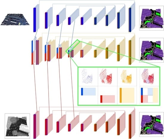
• We develop a composite style fusion network based on Kernel Point Convolution (KPConv), as well as other network architectures, which form part of an ablative study aimed at evaluating the performance of unimodal networks in comparison to the multimodal network (Section 2.2.1). This fusion network is the first to perform a learned feature fusion of 3D point clouds in a fully 3D point convolution-based neural network.
• We propose a unique method for associating hyperspectral point locations with lidar point locations, enabling the generation of a canonical set of points where multimodal features are localized (Section 2.2.2).
• We offer a comprehensive performance analysis of both unimodal and multimodal networks, discussing their results in the context of our proposed hyperspectral representation and fusion implementation (Section 3).

Through these contributions, we strive to not only advance the fusion network to operate entirely in the 3D domain but also to enhance our understanding and processing of hyperspectral and lidar data.

2. Materials and Methods

The contributions of this work are the proposed HSPC representation, KPConv-based [19] multimodal composite fusion style network, and method of multimodal canonical point location generation. To perform the characterization of these contributions, we make specific efforts to prepare the lidar modality from the selected dataset and generate corresponding semantic point labels. Further, we isolate specific unimodal networks to study the efficacy of utilizing the HSPC representations against the standard 2D hyperspectral representation. The dataset, its preprocessing, HSPC generation, model architectures, and canonical point location generation are all described within this section.

2.1. Materials

The selected dataset for this work was provided by the IEEE Geoscience and Remote Sensing Society (GRSS). It was originally provided to participants of the IEEE GRSS 2018 Data Fusion Contest [20] and acquired by the National Center for Airborne Laser Mapping (NACLM) in February 2017. The dataset depicts approximately 5 km${}^2$ of the University of Houston campus and its surrounding areas. It provides three co-registered data modalities: hyperspectral, multispectral lidar, and high-resolution RGB [20] along with semantic pixel labels.

The hyperspectral modality was captured by an ITRES CASI 1500 camera system and covers the 380–1050 nm range over 48 bands at a 1.0 m ground sample distance (GSD) [20]. It was provided as a set of 14 spectrally calibrated and orthorectified image tiles, each 4172 × 1202 pixels [21]. The multispectral lidar modality was acquired with an Optech Belgrade, MT, USA Titan MW camera system across three wavelengths 1550, 1064, and 532 nm at ∼0.5 m GSD [20]. Per each spectral channel, there are 14 point clouds, an intensity raster, and four digital elevation models. A DiMAC ULTRA-LIGHT+ camera system acquired the high-resolution RGB data. It was provided as a set of 14 images of 11,920 × 12,020 pixels in size at a 5 cm GSD [22]. Finally, the semantic pixel labels were developed from OpenStreetMap data as 20 Land Use Land Cover (LULC) classes at a 0.5 m GSD [20]. Of the total 14 multimodal tiles, these semantic labels only cover four. The other 10 tiles were reserved as the test set for the 2018 Data Fusion Contest itself. In this work, we only utilized the hyperspectral, multispectral lidar, and semantic labels. The high-resolution RGB data was excluded.

2.1.1. Preprocessing and Lidar Labeling

In this work, we were concerned with the efficacy of the HSPC representation and its effects on both unimodal networks and multimodal fusion networks. As a result, it was pertinent to ensure that the dataset utilized for the development and characterization of the implemented networks does not present confounding effects on the models’ performance. Thus, preprocessing of the dataset proceeded in the same manner as presented in [8]. In short, we only utilized the 1500 nm multispectral lidar channel, which was collected 3.5° off-nadir; we applied grid subsampling to the lidar data on a 0.5 m grid [19], and subsample the semantic pixels labels with max-pooling. This resulted in a co-registered, geo-registered, and temporally registered dataset with closely matching viewing geometries (overhead at or near nadir) and resolution across all modalities (0.5 m GSD). As noted in [8], this preprocessing does not produce an exact match for the stated data metrics, but it prevents confounding factors from affecting the study of the HSPC representation.

The semantic pixel map provided by the GRSS18 dataset contains 20 distinct LULC along with unlabelled classification. In [8], the spatial distribution of these classes about the dataset was found to be far from equally distributed. This asymmetric distribution of classes makes it difficult to spatially separate the dataset into a training, validation, and testing area from which multimodal samples are drawn. To alleviate this issue, the 20+1 LULC were combined into a set of 5+1 superclasses: foliage, vehicle, vehicle path, human path, and unlabelled exactly as in [8]. Appendix A 

Table A1. GRSS18 class labeling scheme statistics and superclass labeling assignment.

GRSS18 Class	Pixel Count	Percentage of Total	Superclass Assignment
unlabeled	3,712,226	64.773	unlabeled
non-residential buildings	894,769	15.612	buildings
major thoroughfares	185,438	3.236	vehicle path
roads	183,283	3.198	vehicle path
residential buildings	158,995	2.774	buildings
sidewalks	136,035	2.374	human path
stressed grass	130,008	2.268	foliage
evergreen trees	54,322	0.948	foliage
paved parking lots	45,932	0.801	vehicle path
highways	39,438	0.688	vehicle path
healthy grass	39,196	0.684	foliage
railways	27,748	0.484	vehicle path
stadium seats	27,296	0.476	unlabeled
cars	26,289	0.459	vehicle
trains	21,479	0.375	vehicle
deciduous trees	20,172	0.352	foliage
bare earth	18,064	0.315	foliage
crosswalks	6059	0.106	human path
artificial turf	2736	0.048	unlabeled
water	1064	0.019	unlabeled
unpaved parking lots	587	0.010	vehicle path
Total	5,731,136

and

Table A2. Superclass statistics over total imaged area and within training, validation, and test sets.

Superclass	Pixel Count	Percentage of Total	Percentage of TVT Sets
unlabeled	3,743,322	65.316	66.75, 67.33, 56.37
building	1,053,764	18.387	18.45, 11.69, 25.06
vehicle path	482,426	8.418	8.73, 8.52, 6.83
foliage	261,762	4.567	2.05, 4.05, 2.87
human path	142,094	2.479	3.31, 7.18, 7.83
vehicle	47,768	0.833	0.7, 1.23, 1.04

provide an overview of the mapping between classes along with various statics before and after mapping. After the superclass generation was complete, it was possible to spatially separate the dataset into training, validation, and testing regions with closely matching class distributions (see Figure A1).

The GRSS18 dataset provides its semantic labels as a pixel map. The pixels within the semantic labels correspond to the hyperspectral pixels one-to-one. However, no labels are provided which correspond to the lidar points one-to-one. To produce a ground truth labeling of the lidar data for model development and training, we performed the same method presented in [8]. Provided that the hyperspectral, lidar, and semantic pixel labels are co-registered, it is possible to associate all lidar points that fall within a label’s pixel region with that label. To do so, each semantic pixel label is iterated over, and an infinitely tall bounding cuboid is generated for each. All lidar points that fall within a semantic pixel’s cuboid are associated with that label value. The result of this is a lidar point cloud labeling corresponding to the supplied semantic pixel labels. As noted in [8], this does not produce a perfect transfer of labels from the 2D to the 3D domain, but it is sufficient to adequately develop and train networks that utilize the lidar data modality. The largest source of error with this method is due to overhanging structures in the scene, such as foliage and nearby tall structures. Points below overhangs and near the sides of tall structures are incorrectly labeled as the label is applied to the highest point; a result of capturing the hyperspectral data from overhead. This issue is depicted pictorially in the second figure of Decker et al. [8].

2.1.2. Hyperspectral Point Cloud Generation

Section 1 suggests an alternative representation of the hyperspectral modality as a point cloud. This representation is necessary to both ingest and utilize the hyperspectral data within a point convolutional network such as KPConv. Further, this allows for a matching feature representation between hyperspectral and lidar data processing streams of a multimodal fusion network and allays issues noted in [8] with fusing pixel and point convolutional features. To generate this alternative data representation, we projected the hyperspectral data into a higher dimension.

Projecting data into a higher dimension, a basis expansion, is a common technique used in classical machine learning to allow linear classifiers to ingest data that represent non-linear phenomena. We reused this idea for a similar purpose, allowing a segmentation model to work with an alternative data representation. To begin, we first identified that image-type data are comprised of two spatial and one spectral dimension. The spatial dimensions directly correspond to pixel indices. The spectral dimension corresponds to the amount of spectral energy at a given pixel for single or multiple specific wavelengths. On the other hand, point cloud data are comprised of a variable-size set of unordered points in 3D space with irregular spacing and density. Further, at each point, some structural or even spectral information is associated. The most natural and simple translation from pixel-based image-type data to point cloud data is to simply translate pixel locations to points and keep the original association of features at each pixel location. This process is depicted pictorially in Figure 1 for a sample hyperspectral image patch.

While this method of hyperspectral projection achieves a realizable implementation, it makes it difficult to methodologically associate hyperspectral and lidar point locations spatially; a useful feature for multimodal feature fusion is described further in Section 2.2.2. The described method generates a hyperspectral point location at each corresponding pixel location with no defined height (thus requiring a default assumption such as $Z=0$), while all lidar points have some associated height. Thus, hyperspectral points corresponding to locations on objects with height in the scene are vertically distant from the corresponding lidar point(s). To account for this issue, we presented an alteration to the method described in the preceding paragraph by setting the Z values for points as the average height of the lidar points within the pixel’s spatial boundary, essentially mapping the lidar DSM over the hyperspectral points. We labeled the two forms of the HSPCs as the “spectral point cloud” ($Z=0$) and the “structural point cloud” ($Z=DSM$). An example of a hyperspectral sample projection in both formats is provided in Figure 2.

In contrast with the alternative of associating spectral information with each lidar point location, the structural HSPC points contain observed spectral information but interpolated spatial information. Thus, this structural HSPC mainly contains spectral information but also has the ability to be more easily spatially aligned to a corresponding lidar point cloud. We recognize that as a result of associating structural information to the spectral information using the average local lidar point height within the pixel, our technique is limited in its ability to represent complete spatial information in certain locations, such as overhangs or suspended objects where multiple lidar points occupy the same vertical location.

2.1.3. Multimodal Sample Generation

Once preprocessing and HSPC generation were completed, the training, validation, and testing regions of the dataset (see Figure A1) were sub-divided into sets of multimodal samples in the same manner as described in [8]. The primary motivation for this sample generation technique is firstly to produce smaller samples that can properly be ingested by the architectures described in the next section. A secondary motivation is to bolster model comparability between this work and [8] by producing the same set of samples split into the same training, validation, and testing sets. Samples were created by generating a set of spatial boundaries and selecting the data from each modality within each boundary. Boundaries were generated by creating a 128 × 128-pixel region within the pixel coordinate system (hyperspectral image and semantic pixel labels measured in pixel indices) and iterating the boundary every 64 pixels in both the X and Y directions. Further, this operation was performed four times, corresponding to each minimal and maximal corner of the spatial area defining the training, validation, and testing areas. Finally, to slice the values of point cloud-based modalities, the pixel coordinates were translated, based on the defined co-registration, into point coordinates (measured in UTM) and used to select points within that region. This resulted in a combined 980 multimodal samples across the entire training, validation, and testing sets. A single multimodal sample example is depicted in Figure 3.

2.2. Methods

A total of four network architectures were utilized in this work, three unimodal and one multimodal. A summary of their characteristics is provided in

Table 1. Overview of all constructed architectures and their characteristics.

Architecture	Input Modality	CNN Type/ Output Type	Input Data Type	Comprised of
L3D [8]	Single	Point	LI-PC	-
H3D-Flat (HSF)	Single	Point	HS-Spectral	-
H3D-DSM (HSD)	Single	Point	HS-Structural	-
HSD-L3D	Multi	Point	HS-Struct, LI-PC	H3D-DSM, L3D

. One of these architectures (L3D) was originally described in [8], and the other three architectures represent our contribution. These network architectures were selected to determine the efficacy of the HSPC representations toward semantic segmentation and their effects on both unimodal and multimodal fusion networks. To evaluate this, we constructed both unimodal and multimodal fusion networks that make use of the two proposed structural and spectral HSPC representations. Note, a multimodal architecture ingesting lidar point cloud data and the spectral HSPC data was not implemented. This is because when using these two specific modalities, the lidar and hyperspectral point locations are, in height, spatially distant and never undergo mixing during the KPConv operation. As a result, a multimodal architecture using these modalities would, in essence, never be able to generate multimodal features using the method described in Section 2.2.2; this section also provides further information regarding the issue.

The first unimodal architecture L3D [8] ingests lidar point cloud data and predicts a label for each point, i.e., a semantic point cloud. The purpose of this network is to serve as a comparison against the two other unimodal networks which ingest hyperspectral data and as the source of unimodal lidar features for the multimodal fusion network. The next unimodal network H3D-Flat ingests the spectral HSPC and predicts a semantic point cloud. This network serves as a point of comparison against networks that ingest the other hyperspectral data representations. The final unimodal network H3D-DSM ingests the structural HSPC and predicts a semantic point cloud. The purpose of this network is to serve as the final point of comparison for networks that ingest hyperspectral data and also as the source of unimodal hyperspectral features for the HSD-L3D multimodal fusion network. We relied on the results presented in [8] (the H2D network) to obtain the results of a 2D-CNN network that ingests hyperspectral image-type data.

To determine the effect the structural HSPC representation has within multimodal hyperspectral and lidar fusion networks, we introduced the HSD-L3D architecture. This network ingests unimodal features from H3D-DSM and unimodal features from L3D and predicts a semantic point cloud. This serves as a point of comparison for fusion networks that ingest hyperspectral data in the structural point cloud format. We relied on the results presented in [8] to obtain the performance of multimodal fusion networks that ingest hyperspectral data in its native image-type format and lidar data in both its native point cloud format (H2D_L3D in [8]) and its DSM format (H2D_L2D in [8]).

2.2.1. Architectures

All architectures presented in this work are KPConv [19] point convolution-based architectures. The first unimodal point convolution architecture L3D is depicted in the bottom row of Figure 4 in red, and it is constructed exactly as described in [8]. The other two unimodal point convolution architectures H3D-Flat and H3D-DSM, are depicted in the top row of Figure 4 in blue. They are constructed exactly as L3D and themselves the same architecture. Thus, all three unimodal point convolution-based networks have the same architecture and only differ by their input data type; they are the unimodal point cloud processing architecture. The unimodal point cloud processing architecture is a UNet [23] style architecture with four down-sampling encoding sections, a central latent embedding section, and four up-sampling decoding sections. The central embedding section and encoding sections are comprised of a KPConv and a strided KPConv layer. Strided KPConv is analogous to a pooling operation [19]. The decoding sections are comprised of a KPConv nearest neighbor upsampling and a unary KPConv layer. The unary KPConv layer is analogous to a $1\times 1$ pixel convolution. The number of filters in each layer of the encoding section starts at 64 and increases by a factor of 2 in each subsequent layer until the central section, then in the decoding section, decreases by a factor of 2 in each subsequent layer with the final decoding section having the same number of filters as the initial encoding section. A final KPConv layer is at the end of the architecture, which produces an $n\times 1$ class prediction, where n is the number of points in the input.

The multimodal architecture HSD-L3D has three distinct processing streams (rows of Figure 4). The outer (top and bottom) processing streams work only on unimodal data, either hyperspectral or lidar, and are the unimodal networks L3D and H3D-DSM themselves. The inner fusion stream has no input data at the first layer and only accepts fusion connections from the outer unimodal network streams at later layers. Provided the outer unimodal processing streams have already been fully defined in the preceding paragraph, we now describe the central fusion stream architecture here.

The central fusion stream of the HSD-L3D architecture is a UNet-style architecture with four down-sampling encoding sections, a central latent embedding section, and four up-sampling decoding sections. The encoding sections are comprised first of a unimodal feature fusion layer further described in Section 2.2.2 followed by a KPConv and strided KPConv layer. The fusion connections at the start of the encoding layers are directed from the ends of each encoding section of the unimodal processing streams. The central embedding section is comprised of a KPConv and strided KPConv layer. The decoding sections are comprised of a KPConv nearest neighbor upsampling and a unary KPConv layer. The number of filters in each section starts at 128 and increases by a factor of 2 until the central section, then decrease by a factor of 2, with the final decoding section having the same number of filters as the initial encoding section. Further, the input feature count of the first layers within each encoding section is larger than the output value described in the previous section. It is increased by the collective total of the incoming unimodal feature counts; this ensures the multimodal features fit within each encoding section input layer. A final KPConv layer is at the end of the architecture, which produces an $n_f\times 1$ class prediction, where $n_f$ is the number of points in the combined hyperspectral and lidar point cloud inputs to the unimodal processing streams.

2.2.2. Canonical Multimodal Point Creation and Unimodal Feature Fusion

The multimodal fusion architecture HSD-L3D utilizes the unimodal hyperspectral and lidar features generated by H3D-DSM and L3D to generate multimodal features prior to the start of each network section. Unlike pixel convolution-based multimodal fusion networks (e.g., H2D_L2D in [8]), which can naturally concatenate unimodal features along a similar axis, an issue arises when attempting to do the same in a point convolution-based multimodal fusion network. Whereas two sets of pixel features are localized by the same pixel locations (given matching resolutions), two sets of point features may be localized to two different sets of points; see the bottom left-hand panel of Figure 5. Thus, no canonical set of points naturally exists that localizes both of the unimodal features.

Instead of attempting to generate a set of canonical multimodal point locations or selecting a subset of either or both of the hyperspectral or lidar point locations, in this study, we opted to simply combine the point locations from the hyperspectral and lidar point clouds. This set of combined point locations was then deemed the set of canonical multimodal point locations. The motivation behind this decision was to maintain the information contained within the unimodal point features. Had the canonical point locations been selected as a subset of all possible point locations, then some form of interpolation or pooling would be necessary to reduce the features into a dimension amenable to localization at the set of reduced point locations. Thus, keeping all unimodal features and allowing the network to learn this encoding would result in a more informative set of multimodal features.

To properly fuse the features localized by the canonical point locations, the corresponding indices of features from the opposite modality of data were initialized to mean value along the feature dimension (vertical dimension in Figure 5). At the initial layer $l=0$ of the fusion stream of the multimodal networks, this resulted in a fused feature representation. At deeper network layers, the $l-1$ multimodal features must also be incorporated. As a natural consequence of the definition of KPConv and the construction of the initial layer’s canonical points, the correct mapping of the $l-1$ layer’s features and the l layer’s points were already in place. This process is pictorially depicted in the right-hand panels of Figure 5.

The point locations used at each section of a KPConv-based network were pre-computed using grid-subsampling [19]. This means that the unimodal hyperspectral and lidar point locations at each network section are known prior to the network ingesting data and can be used to fully define the set of canonical multimodal point locations. Further, the strided KPConv down-sampling and nearest neighbor up-sampling layers within the fusion stream were referenced to this pre-defined set of canonical point locations. These facts together mean that the multimodal features at the end of the $l-1$ network section were localized to the same set of points at layer l; during encoding, the opposite holds during decoding. In total, this resulted in a unimodal point feature fusion operation that maintained all points and features from both unimodal network connections. Note, that as a result of this method, the semantic point clouds predicted by the multimodal networks could be compared and evaluated from the combined class labels of the corresponding multimodal hyperspectral and lidar input sample.

2.2.3. Graph Pyramid Generation

As mentioned, successive applications of grid subsampling to a given point cloud is necessary to pre-compute the required point locations at which features are localized at each layer/depth within a KPConv-based network. The top three rows of Figure 6 depict the point locations for a single sample prior to ingestion into the H3D-DSM, L3D, and HSD-L3D networks. During the grid subsampling calculation, three other data structures were also instantiated and defined by the results of the operation: down-sampling indices, up-sampling indices, and point neighbor indices. The down-sampling and up-sampling indices indicated many-to-one and one-to-many mappings of points between different depths of the network. They were directly used by strided KPConv and nearest-neighbor upsampling operations to either contract or expand features to a new set of point location(s) during encoding and decoding. The neighbor indices indicate which spatially local points are used during a single given KPConv convolution operation. The fourth-row Figure 6 depicts the set of point neighbors (yellow) for a single point (green) for a single sample passed through the HSD-L3D network. Collectively these pre-computed data structures may be referred to as a graph pyramid.

Calculation of a graph pyramid is straightforward in the case of a unimodal KPConv-based network. However, in the case of a multimodal network such as HSD-L3D, a two-step process must be implemented to ensure proper “mixing” of modalities during the sub-sampling and neighbor index calculations. We completed such a method as follows. In the first step, the input HSPC, and lidar point cloud points were combined into a single data structure to form the canonical set of point locations, and a graph pyramid is created (second row of Figure 6). During the creation of this graph pyramid, the original modalities of individual points were recorded, but the points were allowed to mix. That is, the grid-subsampling operation is not modality-aware and would subsample a mixed-modality set of points into a single new point location for any given grid cell. Further, the neighbor selection operation is also not modality-aware and will select neighbors representing a mixed-modality set of points. In the second step of the process, the recorded originating modality of each point at each depth of the graph pyramid was used to decompose it into two graph pyramids representing the HSPC and lidar graph pyramids for the given input (first and third row of Figure 6).

The resulting multimodal graph pyramid is made up of three distinct graph pyramids, one for each of the unimodal inputs and one for the set of canonical point locations they create. Again, the calculation of the multimodal graph pyramid in this manner is necessary to ensure mixing between the unimodal inputs. Had the unimodal graph pyramids been created first and then combined, the down-sampling, up-sampling, and neighbor indices would only describe relationships between points within the same modality. Thus, KPConv convolution operations would never mix features from opposite modalities within the central fusion stream of the network to generate two multimodal feature sets. For the same reason, this is why a multimodal network ingesting the spectral HSPC and lidar point cloud data is not possible. The grid subsampling operation would rarely find/produce grid cells with a mixed modality of points because the spectral HSPC points have $Z=0$ while the lidar points have some inherent height.

2.2.4. Network Training

We utilized the weighted categorical cross-entropy loss described in [8] for all network optimization. This loss function implements logic to ignore the contribution of unlabeled pixels and points to the calculated loss via masking. Masking was implemented by altering the network class predictions prior to loss calculation by setting the correct prediction for all truly unlabeled pixels or points. Class weights within this loss were calculated as $1.0$ minus the total percentage of their representation in the training set. This weighting alleviated the substantial class imbalance present in the dataset (Table A2).

The single multimodal network was comprised in part of the unimodal networks H3D-DSM and L3D themselves. As a result, training of all unimodal networks proceeded prior to the multimodal network. This allowed the learned parameters of the unimodal networks to be utilized during the training of the multimodal network as the initialization parameters for the hyperspectral and lidar stream of the network. Training of the multimodal network then proceeded by providing multimodal samples to the unimodal input streams, performing a forward pass, accruing gradients, and back-propagating through all reachable layers of the network. That is, the decoding sections of the unimodal network streams have no connections to the central fusion stream, and as a result, weight updates from the loss result at the central fusion stream’s prediction never backpropagate through them.

Sample batching for all networks was performed via the technique described in [19]. This technique stacks input samples along both the point and feature dimensions (essentially localizing all samples in a batch to the same Euclidean space) and relies on the precomputed neighbor indices to identify each sample during training. The total number of points in each of the input samples was also calibrated via the method presented in [8] originally described in [19]. That is, an empirically determined upper bound of 340,000 points per batch was identified, which allows for approximately 16-point cloud samples per lidar batch, 64 point cloud samples per hyperspectral (both the spectral and structural HSPC) batch, and 12 point cloud samples per multimodal batch. These limits were set due to hardware memory limitations.

While the described architectures could ingest entire point cloud samples, they would be limited by small batch size. In order to ensure a larger variability in samples through the KPConv-based networks the point clouds in the multimodal (Figure 3) samples were further sampled. This sampling operation selects a random point within the point cloud, selects a predefined number of points within a rectangular $XY$ region, and uses this as a network input sample. In the case that not enough points are reachable from the randomly selected point, a new point is selected until a sample is found. For the lidar point cloud modality, the number of points was set to 21,250, and for the HSPC modalities, 5300. These values resulted in approximately 1/4 of the entire multimodal sample (Figure 3) being within the generated sample.

All networks were trained for a maximum of 150 epochs, an SGD optimizer with 0.98 momenta, a $1\times {10}^{-2}$ learning rate, a cosine decay based learning rate scheduler, $1\times {10}^{-3}$ weight decay, and gradient norm clipping. During all network training sessions, a monitor was implemented to save the model with the best-observed validation accuracy. After training was complete, the model with the highest validation accuracy was selected for testing and results reporting. All networks were trained on an Nvidia RTX A6000 with 48GB of VRAM under the PyTorch [24] framework with heavy reliance on the PyKeOps [25], easy-kpconv [26], and vision3d-engine [27] libraries. An overview of various model parameters, hyperparameters, and computational requirements is presented in

Table 2. Selected subset of model characteristics and computational requirements. The slight differences between H3D-Flat and H3D-DSM epoch time and memory usage are due to the different sizes of neighbors used during convolution. The reported value of HSD-L3D’s model parameter count includes the decoding sections of the unimodal network streams.

Architecture	# Params	Max Epoch	Opt/LR	Batch Size	Epoch Time	VRAM Mean
L3D	24.3 M	150	SGD/$1\times {10}^{-2}$	16	8.8 min	29 GB
H3D-Flat	24.5 M	150	SGD/$1\times {10}^{-2}$	64	7.2 min	21 GB
H3D-DSM	24.5 M	150	SGD/$1\times {10}^{-2}$	64	6.9 min	20 GB
HSD-L3D	125.7 M	150	SGD/$1\times {10}^{-2}$	12	13.5 min	41 GB

.

2.2.5. Post-Processing

As noted in Section 2.2.1 the L3D network predicts a semantic point cloud localized to the lidar point locations, H3D-Flat and H3D-DSM predict semantic point clouds localized to the HSPC point locations (same points, differing Z values), and HSD-L3D predicts a semantic point cloud localized to both the lidar and hyperspectral point locations. To allow for a fair comparison between all networks presented along with previous works ([21,22,28,29]) the semantic point predictions for the lidar point locations had to be projected into a pixel representation. The semantic point predictions for the HSPC based/localized predictions do not need to be altered because each point has a bijective mapping between pixel locations in the original hyperspectral image. Thus, we utilize the same method described in [8] to project the semantic point label predictions from the L3D network and the lidar prediction component of HSD-L3D network. That is, reversing the operation of labeling the point cloud in the first place as described in Section 2.1.1. Finally, to combine the predictions for each of the multimodal samples back into the original unsliced GRSS18 image format the same method as described in [8] is used; selecting the highest softmax confidence value for all pixel locations.

3. Results

The combined, but not yet projected, test set predictions for all networks are provided in Figure 7. The metrics and statistics calculated from these predictions are provided in

Table 3. Statistics and metrics of combined test sample predictions for all models. Note, predictions are not directly comparable unless they were performed against the same set of point locations. For example, the L3D and HSD-L3D (Lidar) columns are comparable, while the L3D and H3D-Flat predictions are not. A caveat to this is that all HSPC predictions are directly comparable; they share the same set of point locations albeit with different Z values. Further note, as described in Section 2.2.1, L3D was originally described in [8] but retrained in this work provided it is a sub-part of the HSD-L3D network. The best results per point location type are highlighted in bold. The class distribution percentage within the test set is provided beside each class label.

	L3D	HSD-L3D (Lidar)	H3D-Flat	H3D-DSM	HSD-L3D (HSPC)	HSD-L3D (Canonical)
Point Locations	Lidar	Lidar	HSPC	HSPC	HSPC	Canonical
Class Accuracy
building (57.4%)	0.996	0.958	0.735	0.960	0.960	0.958
vehicle path (15.7%)	0.861	0.896	0.861	0.952	0.908	0.897
human path (17.9%)	0.528	0.431	0.271	0.386	0.415	0.430
foliage (6.6%)	0.413	0.635	0.911	0.723	0.550	0.629
vehicle (2.4%)	0.928	0.841	0.241	0.767	0.796	0.837
Statistics
Precision	0.8218	0.7636	0.6881	0.8396	0.7679	0.7640
Recall	0.7451	0.7520	0.6038	0.7579	0.7256	0.7500
F-measure	0.7632	0.7461	0.6009	0.7848	0.7317	0.7452
IoU	0.6461	0.6135	0.4676	0.6695	0.5960	0.6123
Kappa	0.7060	0.7478	0.6017	0.7875	0.7252	0.7462
Balanced Accuracy	0.7451	0.7520	0.6038	0.7579	0.7256	0.7500
Pixel Accuracy	0.8360	0.8536	0.7442	0.8744	0.8385	0.8525

. It is important to note that the values presented in this table are not directly comparable unless they originated from the same input point cloud modality. This is because predictions made against, for example, the lidar point cloud modality are not localized to the same set of points as the HSPC modality. A caveat to this is that all HSPC predictions are directly comparable because they share the same set of point locations albeit with different Z values. In addition, note, in Table 3, the statistics for HSD-L3D are presented against the canonical point locations, lidar point locations, and structural HSPC point locations. This is possible because the canonical set of point locations can easily be decomposed into the lidar and hyperspectral contributions as a result of the pre-computed graph pyramid input (Section 2.2.3). We present these metrics and statistics to illustrate the models’ performance against their input, in the proceeding paragraphs, we also present their projected predictions for inter-model comparison.

First, we compare the two predictions from L3D and HSD-L3D (Lidar) against the lidar point cloud locations. The marginal balanced and pixel accuracy improvements of the HSD-L3D (Lidar) prediction over the L3D prediction provides weak evidence that the incorporation of the structural HSPC information within the multimodal network is effective. Further, we note the differences in the per-class accuracy against the vehicle class. The L3D network moderately outperformed the HSD-L3D, and thus, we recognize that the incorporation of the structural point cloud information within the multimodal network, while effective overall, could introduce some ambiguity toward specific classes. In this case, a correct prediction on the vehicle class may be the most reliant on structural information (in relation to the other classes) for proper prediction given the highly variable spectral information vehicles present.

We may also compare the three predictions from the H3D-Flat, H3D-DSM, and HSD-L3D (HSPC) models against the HSPC point locations. The overall under-performance of the H3D-Flat network is directly attributed to the 2D nature of the spectral HSPC input. This modality does not provide structural information and results in many of the KPConv kernels/filters going under-utilized. Despite this, the model was still able to produce non-trivial performance. Interestingly, the rooftop parking garage structure on the left-hand side of the test area (top left subplot of Figure 8), which is subjectively incorrectly labeled entirely as the building class, was best segmented by this model (which in turn negatively affected its reported accuracy).

The moderate increase in balanced and pixel accuracy improvements of the H3D-DSM network over the multimodal network is mainly attributed to the greatly increased training cost of the multimodal network. The H3D-DSM, and all other unimodal networks, are smaller architectures in terms of both number of parameters and input point cloud size. As a result, they are faster to train and can be fed much larger batch sizes. This allows for a greater number of epochs and sample variety per unit of computational cost. Further, the structural HSPC itself is already a multimodal data product and provides a subjectively reasonable and pre-defined association of hyperspectral and lidar features in the spatial domain. As a result, this model may have been able to rely on this fact, whereas the multimodal network had to learn a useful mapping between its input unimodal feature sets.

The combined and projected (Section 2.2.5) test set predictions for all networks are provided in Figure 8. The metrics and statistics from these predictions are provided in

Table 4. Statistics and metrics of the combined test sample predictions after projection to the $XY$ plane and ground truth label pixel locations. All values are directly comparable. Further, the predictions originally made against the HSPC modalities did not change as a result of the method of HSPC creation; pixel $XY$ values are equal to point $XY$ values for all HSPC representations. The first six columns represent models trained in this work. The final four columns represent previous work. The final column represents the translated [8] (accounting for superclass conversion; Section 2.1.1) results of Li et al. [29] against the GRSS18 dataset. We rely on the short-hand naming of the H3D-Flat (HSF) and H3D-DSM (HSD) naming in the table for spacing. The best results are highlighted in bold.

				HSD-L3D
	L3D	HSF	HSD	Lidar	Hyper	Canon	H2D [8]	H2D_L2D [8]	H2D_L3D [8]	Li [29]
Class Accuracy
building	0.997	0.735	0.960	0.959	0.960	0.959	0.918	0.992	0.897	0.899
vehicle path	0.855	0.861	0.952	0.891	0.908	0.877	0.695	0.840	0.863	0.720
human path	0.434	0.271	0.386	0.347	0.415	0.308	0.482	0.472	0.459	0.508
foliage	0.335	0.911	0.723	0.565	0.550	0.561	0.932	0.856	0.934	0.860
vehicle	0.876	0.241	0.767	0.758	0.796	0.756	0.415	0.946	0.385	0.863
Statistics
Precision	0.8198	0.6881	0.8396	0.7729	0.7679	0.7652	0.825	0.899	0.854	-
Recall	0.6994	0.6038	0.7579	0.7040	0.7256	0.6922	0.831	0.897	0.844	-
F-measure	0.7277	0.6009	0.7848	0.7178	0.7317	0.7064	0.825	0.894	0.842	-
IoU	0.6039	0.4676	0.6695	0.5799	0.5960	0.5686	0.720	0.830	0.745	-
Kappa	0.6742	0.6017	0.7875	0.7079	0.7252	0.6959	0.730	0.838	0.756	-
Balanced Acc	0.6994	0.6038	0.7579	0.7040	0.7256	0.6922	0.688	0.821	0.708	0.768
Pixel Accuracy	0.8078	0.7442	0.8744	0.8214	0.8385	0.8149	0.831	0.897	0.844	0.819

. This table further provides the results of the H2D unimodal traditional pixel CNN network ingesting hyperspectral images and the H2D_L2D multimodal traditional pixel CNN network ingesting hyperspectral images and lidar DSM data originally described in Decker et al. [8]. In the figure and table, all predictions are directly comparable because they are all localized to the same label pixel locations. Note, the metrics and statistics of the HSPC ingesting models did not change because of the bijective mapping between the HSPC point locations and label pixel locations. We also comment on the overall decrease in the reported statistics for non-HSPC-based models (L3D, HSD-L3D (Lidar), and HSD-L3D (Canonical)). This is a result of the in-exacting process of projecting and interpolating the predicted labels localized to their respective point locations to a regularly gridded and smaller set of pixel locations. The largest inaccuracy is in the selection of a label from a set of labels that fall within a single pixel location. This phenomenon is closely related to issues with generating the lidar point cloud labels in the first place (Section 2.1.1).

First, we compare the results of the unimodal network predictions L3D, H3D-Flat, H3D-DSM, and H2D [8]; note that Table 4 uses the shorthand naming for H3D-Flat (HSF) and H3D-DSM (HSD). In terms of both balanced and pixel accuracy, the HSD network outperforms all other unimodal networks. We attribute this to the same reasoning presented for H3D-DSM’s performance when reviewing the unprojected predictions, the structural HSPC itself is already a multimodal data product and provides a subjectively reasonable and pre-defined association of hyperspectral and lidar features. Further, all other unimodal networks have no source of multimodal information. The structural HSPC provides some structural information by definition, and thus provides multimodal information. If we then compare all other unimodal networks, we find that the H2D [8] outperforms all others in terms of balanced and pixel accuracy.

H2D weakly outperforms L3D, from this, we have moderate evidence that the amount of predictive information contained within the hyperspectral and lidar modalities are approximately equal. This is further evidence and expounded upon by comparing the per-class accuracies of the L3D and H2D networks to all other results. We find that the L3D and H2D networks collectively contain the highest number of best results for per-class accuracies. As may be assumed the L3D network ranks highest for more structurally defined classes like the building and vehicle class, while the H2D network ranks highest for the more spectrally defined classes human path and foliage.

Broadening the scope of the comparison to include the decomposed HSD-L3D lidar and hyperspectral components, we find the same performance rankings hold. These results also present further evidence of the approximately equal predictive power of the two modalities. This can be seen in the closely matched balanced and pixel accuracy results of the HSD-L3D (Lidar) and HSD-L3D (HSPC) models. Had one modality provided richer information from which the segmentations could be predicted, then we would expect the contribution to the overall performance from the components of a multimodal model like HSD-L3D to be further separated.

A holistic review of the multimodal network performance incorporates the results of the H2D_L2D and H2D_L3D from Decker et al. With these results, we find that the H2D_L2D network moderately outperformed all other multimodal networks described here and within Decker et al. We attribute this result to the overall difficulty in creating and training mixed modality fusion-based neural networks specifically fusing dissimilar modalities and the computational cost of training KPConv-based networks. When expanding past the result of this work and [8], using the superclass translated result presented in Table 3 of [8], we find that all three multimodal networks described here and in [8] provide competitive performance to existing approaches.

4. Discussion

The fusion of dissimilar data modalities in neural networks presents a significant challenge. Striking a balance between adapting data representations to fit a network architecture, as demonstrated in this work, and adjusting a network architecture to accommodate data representation [8] is crucial. While the fusion of hyperspectral images with lidar DSM data has been extensively studied, we have identified and explored alternative balancing points. Our findings reveal that these points exist, offer competitive results, and have the potential to achieve state-of-the-art performance in semantic segmentation of multimodal hyperspectral and lidar remote sensing datasets with further research.

It is important to recognize the inherent limitations of our methods and contributions. While the results yielded by our newly introduced HSPC representations and the KPConv-based fusion network are promising, certain challenges are present. The first limitation pertains to the adaptation of data representations to fit the network architecture. This might inadvertently result in the loss of some critical details from the original data. In this work, this issue surfaced in the context of hyperspectral pixels that contained multiple lidar points within their vertical column. These were translated into hyperspectral points based on the average height of the lidar points, leading to an inherent displacement. Consequently, the resultant hyperspectral point lay at an indeterminate vertical distance away from the exact point from which its spectrum was initially received.

The second limitation relates to the computational intensity of our proposed network architecture. While the unimodal KPConv-based networks can be accommodated by less powerful, consumer-grade hardware, (albeit at the cost of increased processing time), the more resource-intensive fusion network poses a greater challenge. Its requirements often exceed the computational resources, particularly GPU VRAM, readily available to an individual researcher. These issues represent crucial areas for further refinement in future research.

Despite these limitations, we envision the following path toward this goal of continued research:

• Harness the power of LiDAR data in its native, information-rich point cloud format. Over the past decade, remarkable progress has been made in point cloud processing networks research [30], with novel processing methodologies and network architectures emerging at a rapid pace. This progress should be extended to the field of multimodal remote sensing. The encouraging results of the L3D network further support this notion, as the point cloud processing-based network L3D (trained in this work) achieves a 9% higher pixel accuracy than the lidar DSM network L2D. Continued exploration of point cloud processing methodologies promises to yield enhanced performance.
• Employ and integrate advanced neural network architectures and components. This work has primarily focused on traditional pixel and point-based convolutions. However, more sophisticated pixel and point convolution-based architectures hold the potential to improve performance. For instance, pixel-based convolution can be enhanced with residual layers or attention mechanisms, which are commonly employed in practice. Similarly, KPConv can be augmented with residual layers or deformable kernels. Another potential modification for KPConv, not yet implemented, is a 2D mode of operation. This would facilitate the processing of images (after being converted into spectral point clouds as described in Section 2.1.2) and make full use of the kernel points set, requiring only structural information for point feature fusion to co-locate features spatially.

In conclusion, this work has introduced two HSPC representations and a novel point convolution-based composite fusion neural network that leverages these HSPC representations. Our results demonstrate the efficacy of these representations in both unimodal and multimodal networks and show that the proposed multimodal network delivers competitive performance compared to previous research. This work represents a significant stride towards the development of fusion neural networks capable of processing both native image type data and point cloud data, specifically in the realm of multimodal remote sensing. We recognize the limitations associated with point convolution neural networks like KPConv, including their substantial computational cost and added complexity. However, these challenges are difficult to overcome given the inherently large size and dimensionality of point cloud data. In light of these findings, our work paves the way for innovative approaches to multimodal remote sensing exploitation, unlocking new possibilities for enhanced data analysis and interpretation.

References

1. Kuras, A.; Brell, M.; Rizzi, J.; Burud, I. Hyperspectral and Lidar Data Applied to the Urban Land Cover Machine Learning and Neural-Network-Based Classification: A Review. Remote Sens. 2021, 13, 3393. [Google Scholar] [CrossRef]
2. Singh, M.K.K.; Mohan, S.; Kumar, B. Fusion of hyperspectral and LiDAR data using sparse stacked autoencoder for land cover classification with 3D-2D convolutional neural network. J. Appl. Remote Sens. 2022, 16, 034523. [Google Scholar] [CrossRef]
3. Tang, J.; Liang, J.; Yang, Y.; Zhang, S.; Hou, H.; Zhu, X. Revealing the Structure and Composition of the Restored Vegetation Cover in Semi-Arid Mine Dumps Based on LiDAR and Hyperspectral Images. Remote Sens. 2022, 14, 978. [Google Scholar] [CrossRef]
4. Nguyen, C.; Sagan, V.; Bhadra, S.; Moose, S. UAV Multisensory Data Fusion and Multi-Task Deep Learning for High-Throughput Maize Phenotyping. Sensors 2023, 23, 1827. [Google Scholar] [CrossRef] [PubMed]
5. Kuras, A.; Brell, M.; Liland, K.H.; Burud, I. Multitemporal Feature-Level Fusion on Hyperspectral and LiDAR Data in the Urban Environment. Remote Sens. 2023, 15, 632. [Google Scholar] [CrossRef]
6. Wu, H.; Dai, S.; Liu, C.; Wang, A.; Iwahori, Y. A Novel Dual-Encoder Model for Hyperspectral and LiDAR Joint Classification via Contrastive Learning. Remote Sens. 2023, 15, 924. [Google Scholar] [CrossRef]
7. Lu, T.; Ding, K.; Fu, W.; Li, S.; Guo, A. Coupled adversarial learning for fusion classification of hyperspectral and LiDAR data. Inf. Fusion 2023, 93, 118–131. [Google Scholar] [CrossRef]
8. Decker, K.T.; Borghetti, B.J. Composite Style Pixel and Point Convolution-Based Deep Fusion Neural Network Architecture for the Semantic Segmentation of Hyperspectral and Lidar Data. Remote Sens. 2022, 14, 2113. [Google Scholar] [CrossRef]
9. Chen, A.; Wang, X.; Zhang, M.; Guo, J.; Xing, X.; Yang, D.; Zhang, H.; Hou, Z.; Jia, Z.; Yang, X. Fusion of LiDAR and Multispectral Data for Aboveground Biomass Estimation in Mountain Grassland. Remote Sens. 2023, 15, 405. [Google Scholar] [CrossRef]
10. Brell, M.; Segl, K.; Guanter, L.; Bookhagen, B. 3D hyperspectral point cloud generation: Fusing airborne laser scanning and hyperspectral imaging sensors for improved object-based information extraction. ISPRS J. Photogramm. Remote Sens. 2019, 149, 200–214. [Google Scholar] [CrossRef]
11. Zhang, L.; Jin, J.; Wang, L.; Rehman, T.U.; Gee, M.T.; Zhang, L.; Jin, J.; Wang, L.; Rehman, T.U.; Gee, M.T. Elimination of Leaf Angle Impacts on Plant Reflectance Spectra Using Fusion of Hyperspectral Images and 3D Point Clouds. Sensors 2022, 23, 44. [Google Scholar] [CrossRef] [PubMed]
12. Mitschke, I.; Wiemann, T.; Igelbrink, F.; Hertzberg, J. Hyperspectral 3D Point Cloud Segmentation Using RandLA-Net; Springer Nature Switzerland: Cham, Switzerland, 2023; pp. 301–312. [Google Scholar] [CrossRef]
13. Goodfellow, I.J.; Pouget-Abadie, J.; Mirza, M.; Xu, B.; Warde-Farley, D.; Ozair, S.; Courville, A.; Bengio, Y. Generative Adversarial Networks. In Proceedings of the 27th International Conference on Neural Information Processing Systems (NIPS 2014), Montreal, QC, Canada, 8–13 December 2014; pp. 2672–2680. [Google Scholar]
14. Jaderberg, M.; Simonyan, K.; Zisserman, A.; Kavukcuoglu, K. Spatial Transformer Networks. In Proceedings of the Advances in Neural Information Processing Systems, Montreal, QC, Canada, 7–12 December 2015; Volume 2015, pp. 2017–2025. [Google Scholar]
15. Zhang, M.; Li, W.; Zhang, Y.; Tao, R.; Du, Q. Hyperspectral and LiDAR Data Classification Based on Structural Optimization Transmission. IEEE Trans. Cybern. 2022, 53, 3153–3164. [Google Scholar] [CrossRef] [PubMed]
16. Zhang, Y.; Zhang, M.; Li, W.; Wang, S.; Tao, R. Language-Aware Domain Generalization Network for Cross-Scene Hyperspectral Image Classification. IEEE Trans. Geosci. Remote Sens. 2023, 61, 1–12. [Google Scholar] [CrossRef]
17. Piramanayagam, S.; Saber, E.; Schwartzkopf, W.; Koehler, F. Supervised Classification of Multisensor Remotely Sensed Images Using a Deep Learning Framework. Remote Sens. 2018, 10, 1429. [Google Scholar] [CrossRef] [Green Version]
18. Karpathy, A.; Toderici, G.; Shetty, S.; Leung, T.; Sukthankar, R.; Li, F.F. Large-scale video classification with convolutional neural networks. In Proceedings of the IEEE Computer Society Conference on Computer Vision and Pattern Recognition, Columbus, OH, USA, 23–28 June 2014; IEEE Computer Society: Washington, DC, USA; pp. 1725–1732. [Google Scholar] [CrossRef] [Green Version]
19. Thomas, H.; Qi, C.R.; Deschaud, J.E.; Marcotegui, B.; Goulette, F.; Guibas, L.J. KPConv: Flexible and Deformable Convolution for Point Clouds. In Proceedings of the IEEE International Conference on Computer Vision, Seoul, Republic of Korea, 27 October–2 November 2019; Volume 2019, pp. 6410–6419. [Google Scholar]
20. Xu, Y.; Du, B.; Zhang, L.; Cerra, D.; Pato, M.; Carmona, E.; Prasad, S.; Yokoya, N.; Hansch, R.; Le Saux, B. Advanced multi-sensor optical remote sensing for urban land use and land cover classification: Outcome of the 2018 IEEE grss data fusion contest. IEEE J. Sel. Top. Appl. Earth Obs. Remote Sens. 2019, 12, 1709–1724. [Google Scholar] [CrossRef]
21. Hong, D.; Chanussot, J.; Yokoya, N.; Kang, J.; Zhu, X.X. Learning-Shared Cross-Modality Representation Using Multispectral-LiDAR and Hyperspectral Data. IEEE Geosci. Remote Sens. Lett. 2020, 17, 1470–1474. [Google Scholar] [CrossRef] [Green Version]
22. Xu, Y.; Du, B.; Zhang, L. Multi-source remote sensing data classification via fully convolutional networks and post-classification processing. In Proceedings of the International Geoscience and Remote Sensing Symposium (IGARSS), Valencia, Spain, 22–27 July 2018; Institute of Electrical and Electronics Engineers Inc.: Manhattan, NY, USA; Volume 2018, pp. 3852–3855. [Google Scholar] [CrossRef]
23. Ronneberger, O.; Fischer, P.; Brox, T. U-Net: Convolutional Networks for Biomedical Image Segmentation. In Medical Image Computing and Computer-Assisted Intervention—MICCAI 2015; Springer: Cham, Switzerland, 2015. [Google Scholar]
24. Paszke, A.; Gross, S.; Massa, F.; Lerer, A.; Bradbury, J.; Chanan, G.; Killeen, T.; Lin, Z.; Gimelshein, N.; Antiga, L.; et al. PyTorch: An Imperative Style, High-Performance Deep Learning Library. In Advances in Neural Information Processing Systems 32; Wallach, H., Larochelle, H., Beygelzimer, A., d’Alché-Buc, F., Fox, E., Garnett, R., Eds.; Curran Associates, Inc.: Red Hook, NY, USA, 2019; pp. 8024–8035. [Google Scholar]
25. Feydy, J.; Glaunès, J.; Charlier, B.; Bronstein, M. Fast geometric learning with symbolic matrices. Adv. Neural Inf. Process. Syst. 2020, 33, 14448–14462. [Google Scholar]
26. GitHub-qinzheng93/Easy-KPConv: A More Easy-to-Use Implementation of KPConv. Available online: https://github.com/qinzheng93/vision3d-engine (accessed on 3 January 2022).
27. GitHub-qinzheng93/Vision3d-Engine: Vision3d-Engine: An Easy-to-Use Yet Powerful Training Engine from Vision3d. Available online: https://github.com/qinzheng93/Easy-KPConv (accessed on 3 January 2022).
28. Cerra, D.; Pato, M.; Carmona, E.; Azimi, S.M.; Tian, J.; Bahmanyar, R.; Kurz, F.; Vig, E.; Bittner, K.; Henry, C.; et al. Combining deep and shallow neural networks with ad hoc detectors for the classification of complex multi-modal urban scenes. In Proceedings of the International Geoscience and Remote Sensing Symposium (IGARSS), Valencia, Spain, 22–27 July 2018; Volume 2018, pp. 3856–3859. [Google Scholar] [CrossRef] [Green Version]
29. Li, C.; Tang, X.; Shi, L.; Peng, Y.; Tang, Y. A Two-Staged Feature Extraction Method Based on Total Variation for Hyperspectral Images. Remote Sens. 2022, 14, 302. [Google Scholar] [CrossRef]
30. Guo, Y.; Wang, H.; Hu, Q.; Liu, H.; Liu, L.; Bennamoun, M. Deep Learning for 3D Point Clouds: A Survey. arXiv 2019, arXiv:1912.12033. [Google Scholar] [CrossRef] [PubMed]
Figure 1. Simple method of initial 2D hyperspectral image projection into a 3D hyperspectral point cloud. (Left) A 2D hyperspectral image with pixel locations identified by blue points. Note the hyperspectral image in the plot has many more actual pixels than depicted. (Right) A 3D hyperspectral point cloud is created by translating pixels to point locations (blue) and associating pixel spectrum values at the new point locations 1-to-1.
Applsci 13 08210 g001
Figure 2. Example of GRSS18 hyperspectral data after undergoing the two proposed projection methods. (Left) The hyperspectral sample is projected by the simple method where the point heights are initialized to Z = 0 , i.e., the spectral point cloud. (Right) The hyperspectral sample is projected by a more complex method where the point heights are initialized to the lidar DSM, i.e., the structural point cloud.
Applsci 13 08210 g002
Figure 3. Example of a single multimodal sample after preprocessing, hyperspectral point cloud generation, and sample slicing. (Top Row) The semantic pixel labels, semantic point labels, and lidar points are colored by Z-height. (Bottom Row) The hyperspectral image, spectral point cloud ( Z = 0 ), and structural point cloud ( Z = D S M ).
Applsci 13 08210 g003
Figure 4. All four KPConv-based architectures HSF, HSD, L3D, and HSD-L3D. (Top row, blue) The architecture of the HSF and HSD unimodal networks. These architectures ingest either of the HSPC representations and predict a semantic point map against the hyperspectral point locations. (Bottom row, red) The architecture of the L3D unimodal network. This architecture ingests lidar point cloud data and predicts a semantic point map against the lidar point locations. (Center row, orange) The architecture of the HSD-L3D network. This network ingests unimodal features from the HSD and L3D networks via the vertical fusion connections, generates and learns multimodal features, and predicts a semantic point map against the canonical point locations.
Applsci 13 08210 g004
Figure 5. Process of canonical multimodal point location creation and unimodal feature fusion. (Top Left) The HSD-L3D network, which utilizes this method for feature fusion. (Top Right) An enlarged view of a single layer-stack of the central fusion stream of the network where unimodal feature fusion takes place. (Bottom Left) Point locations and feature representations of the unimodal and multimodal features prior to feature fusion. (Bottom Right) Canonical point locations and feature representation resulting from the creation and fusion process. Note, the multimodal point locations and features are only present after the first layer of the network. When present, these multimodal point locations are passed from the prior unimodal layers ( l 1 ) of the network.
Applsci 13 08210 g005
Figure 6. A graph pyramid from a single multimodal sample passed through the HSD-L3D network. (Top 3 Rows) The structural HSPC, lidar, and canonical point locations at each layer of the HSD-L3D network. As described in Section 2.2.2, the central canonical multimodal point locations are the combination of unimodal point locations at each respective depth of the network streams. (Fourth Row) A visual representation of the neighbor indices (yellow points) with respect to a single point (green) during a single KPConv convolution operation.
Applsci 13 08210 g006
Figure 7. Combined test sample predictions over the entire test set area for all models. Note, predictions are shown against the point locations against which they were generated; denoted in parenthesis in subplot naming. (Row 1, Column 1) Ground truth point cloud labels for the structural HSPC. (Row 1, Column 2) Ground truth point cloud labels for the lidar modality. (Row 2, Column 1) L3D prediction. (Row 3, Column 1) H3D-Flat prediction. (Row 4, Column 1) H3D-DSM prediction. (Row 2, Column 2) HSD-L3D prediction. (Row 3, Column 2) Structural HSPC component of HSD-L3D prediction. (Row 4, Column 2) Lidar point cloud component HSD-L3D prediction.
Applsci 13 08210 g007
Figure 8. Combined test sample predictions over the entire test set area for all models. Note, all predictions have been projected into the X Y plane and localized to the set of pixel locations of the pixel labels as described in Section 2.2.5. As a result, all predictions are directly comparable. (Row 1, Column 1) False color hyperspectral image of the labeled test set area. (Row 1, Column 2) Ground truth pixel labels. (Row 2, Column 1) L3D prediction. (Row 3, Column 1) H3D-Flat prediction. (Row 4, Column 1) H3D-DSM prediction. (Row 2, Column 2) HSD-L3D prediction. (Row 3, Column 2) Structural HSPC component of HSD-L3D prediction. (Row 4, Column 2) Lidar point cloud component HSD-L3D prediction.
Applsci 13 08210 g008