Velocity Control of a Multi-Motion Mode Spherical Probe Robot Based on Reinforcement Learning

Abstract

As deep space exploration tasks become increasingly complex, the mobility and adaptability of traditional wheeled or tracked probe robots with high functional density are constrained in harsh, dangerous, or unknown environments. A practical solution to these challenges is designing a probe robot for preliminary exploration in unknown areas, which is characterized by robust adaptability, simple structure, light weight, and minimal volume. Compared to the traditional deep space probe robot, the spherical robot with a geometric, symmetrical structure shows better adaptability to the complex ground environment. Considering the uncertain detection environment, the spherical robot should brake rapidly after jumping to avoid reentering obstacles. Moreover, since it is equipped with optical modules for deep space exploration missions, the spherical robot must maintain motion stability during the rolling process to ensure the quality of photos and videos captured. However, due to the nonlinear coupling and parameter uncertainty of the spherical robot, it is tedious to adjust controller parameters. Moreover, the adaptability of controllers with fixed parameters is limited. This paper proposes an adaptive proportion–integration–differentiation (PID) control method based on reinforcement learning for the multi-motion mode spherical probe robot (MMSPR) with rolling and jumping. This method uses the soft actor–critic (SAC) algorithm to adjust the parameters of the PID controller and introduces a switching control strategy to reduce static error. As the simulation results show, this method can facilitate the MMSPR’s convergence within 0.02 s regarding motion stability. In addition, in terms of braking, it enables an MMSPR with random initial speed brake within a convergence time of 0.045 s and a displacement of 0.0013 m. Compared with the PID method with fixed parameters, the braking displacement of the MMSPR is reduced by about 38%, and the convergence time is reduced by about 20%, showing better universality and adaptability.

1. Introduction

The exploration of extraterrestrial planets is widely regarded as a cutting-edge pursuit in contemporary science and technology, owing to its remarkable foresight and innovative potential. However, since the planets have much uncertainty, it is dangerous for humans to explore them directly. Therefore, replacing humans with unmanned detection equipment (such as mobile robots and detection vehicles) is the main development trend in deep space exploration missions.

Due to their geometrically symmetrical structure, spherical robots have better balance and flexibility [1]. Thus, they are highly resistant to the rollover problems that wheeled or tracked robots suffer. Consequently, they have attracted many researchers and have been widely used in the detection of unknown environments [2], environmental monitoring [3,4], surveillance [5], and other fields [6]. Based on the single-motion mode [7,8,9], researchers have gradually developed spherical robots with multi-motion modes, such as rolling and jumping, rolling and crawling, and others [10,11,12,13]. The multi-motion mode further expands the application of spherical robots in environmental detection tasks. During exploration missions, the spherical robot is commonly outfitted with specialized, internally contained optical functional modules designed to capture images and record video. However, owing to structural discrepancies in the MMSPR, its mass distribution is non-uniform. Any deviation in the MMSPR’s movement during the rolling process could trigger an excessive motion in its rotational direction, resulting in a disruption of the robot’s postural stability. This instability could severely impact the quality of photos and videos captured during exploration missions. Additionally, such motion instability can exacerbate the force exerted on the optical modules and other associated equipment, leading to reduced service life and higher chances of maintenance costs. Therefore, maintaining the motion stability of the MMSPR during its rolling process is of great significance. In addition, the MMSPR could switch to jump mode to cross obstacles while performing exploration missions. In such a situation, it is crucial for the MMSPR to brake rapidly and adjust its postures after landing to allow for user intervention for the next course of action. This prevents the MMSPR from reentering obstacles, ensuring the efficiency and safety of the task. In conclusion, the successful implementation of the MMSPR in deep space exploration hinges on addressing two critical issues: motion stability and rapid braking.

The spherical robot is a strong-coupled and underactuated system with nonholonomic constraints [14], which poses considerable challenges to its control. Moreover, the unmodeled dynamics of the system and environmental measurement errors will affect the closed-loop stability of the system [15]. There are few studies on the postures control and trajectory tracking of spherical robots. The primary control algorithms used include the sliding mode algorithm [16,17,18], the PID algorithm [19], the fuzzy algorithm [20,21], and others [22,23]. Kayacan decoupled the spherical robot into two subsystems and designed a feedback controller with fuzzy logic to achieve linear motion [24]. The fuzzy controller enhanced the system’s adaptability to nonlinear characteristics and uncertainties, resulting in superior control performance compared to traditional proportion–differentiation (PD) control. Kamis designed a fuzzy PD controller to address the trajectory tracking issue of a spherical robot [25]. The controller uses fuzzy logic to adjust the parameters of the PD controller, which effectively eliminates the overshoot and improves the stability time, thus ensuring more accurate control of the robot’s position. Considering the asymmetry of the spherical robot prototype, Zhang proposed an adaptive hierarchical sliding mode controller (AHSMC) [26]. This controller combines hierarchical sliding mode control (HSMC) with adaptive laws to address the spherical robot’s balance control and velocity control during motion.

The PID algorithm is extensively used in industrial applications, and its parameter tuning is critical to achieving effective control. However, it becomes challenging to obtain the desired control effect when dealing with nonlinear and strongly coupled systems by merely setting fixed controller parameters. Furthermore, the controller’s performance may deteriorate if the system’s parameters exceed the controller’s range [27], indicating poor adaptability and generalization. Reinforcement learning is a method to find the optimal solution from the interaction between the agent and the environment [28]. Combining it with the traditional PID algorithm can improve the generalization and adaptability of a PID controller. Zheng proposed a PID controller based on reinforcement learning to enhance the trajectory tracking performance in a quadrotor [29]. Combining the proximal policy optimization (PPO) algorithm with the traditional PID controller, this method has improved response time, reduced overshoot, minimized control errors, enhanced stability, and strong anti-interference capabilities compared with the traditional PID controller. Wang developed a Q-learning PID controller for trajectory tracking in mobile robots [30]. This controller adjusts the output of the PID controller with the output from Q-learning, achieving precise trajectory tracking. Guan introduced an adaptive PID controller based on radial basis function (RBF) networks for complex nonlinear systems [31]. The controller utilizes the RBF network to adaptively adjust the PID controller’s parameters based on the system’s current state errors, which achieves stable control without system modeling in advance. Park adjusted proportion–integration (PI) parameters online through reinforcement learning so that the vehicle could follow the target more accurately [32]. According to the above research, the combination of reinforcement learning and the traditional PID controller improves the performance of control systems, which is useful for practical engineering applications.

Due to the nonlinear coupling and parameter uncertainty in the dynamic model of the MMSPR, it is complex to adjust the controller parameters manually. Furthermore, controllers with fixed parameters have constrained adaptability. Considering the requirements of deep space exploration tasks and the integrated optical functional modules, this article researches the control method for the MMSPR. The aim is to address the challenges concerning the robot’s motion stability during the rolling process and rapid braking after crossing obstacles. Moreover, the feasibility and effectiveness of the controller proposed in this paper are substantiated through simulation.

The structure of this paper is organized as follows. Section 2 introduces the mechanical design and dynamic model of the spherical robot. Section 3 describes the design of the adaptive PID controller based on reinforcement learning. Section 4 shows and discusses the simulation results in motion stability and rapid braking situations. Finally, Section 5 provides conclusions and future research prospects.

2. Materials and Methods

2.1. Design of the Structure

The structure of MMSPR discussed in this paper is shown in Figure 1, which comprises the spherical shell, the rolling drive module, and the jumping drive module. The shell comprises two hemispheres connected by flanges, forming a closed spherical environment. The rolling drive module consists of two racks and three motors, which are used to drive the robot forward, backward, and steer. The jumping drive module primarily consists of a mechanism box and two six-bar mechanisms, which enable the robot to jump. The specific structural design can be found in our previous work [11].

2.2. Dynamic Modeling

The dynamic model of MMSPR in this paper is based on the following assumptions:

• During movement, MMSPR rolls without slipping, and its mass is decomposed into the mass of the shell and the pendulum: $M_s$, $m_p$;
• The centroid of MMSPR coincides with its geometric center;
• The two degrees of freedom do not mutually interfere, and the longitudinal axis does not rotate.

The schematic diagram of MMSPR during rolling is shown in Figure 2a. Specifically, $O_A$, $O_B$, and $O_C$ represent the coordinate systems $O_A-X_A{Y}_A{Z}_A, O-X_B{Y}_B{Z}_B$, and $O-X_C{Y}_C{Z}_C$, and $O_A$ is the world coordinate system. $O_B$ is the coordinate system fixed at the geometric center of the sphere, which can only translate relative to $O_A$. Additionally, $O_C$ is the coordinate system fixed at the geometric center of the sphere, which can only rotate relative to $O_A$. $R$ and $L$ represent sphere’s radius and the pendulum’s length, respectively. $\theta$ and $\varphi$ represent the rolling angles of MMSPR along its $X_B$ and $Y_B$. $\alpha$ and $\beta$ refer to the rotation angles of the pendulum around the $X_B$ and $Y_B$. ${\tau }_x$ and ${\tau }_y$ are the driving torques acting on the $X_B$ and $Y_B$.

To facilitate the controller design, MMSPR’s system needs to be decoupled. Referring to Kayacan [24], we decoupled the robot into the forward motion and the steering motion (Figure 2b,c). According to the Lagrange equation, taking the state variable $x={\left[\begin{array}{cccc}\theta & \alpha & \varphi & \beta \end{array}\right]}^T$, the dynamic model of MMSPR can be formulated as:

$$\begin{array}{c}M\left(x\left(t\right)\right)\ddot{x}\left(t\right)+V\left(x\left(t\right),\dot{x}\left(t\right)\right)=u\left(t\right)\\ \left[\begin{array}{cccc}{M}_{11}& M_{12}& M_{13}& M_{14}\\ M_{21}& M_{22}& M_{23}& M_{24}\\ M_{31}& M_{32}& M_{33}& M_{34}\\ M_{41}& M_{42}& M_{43}& M_{44}\end{array}\right]\left[\begin{array}{c}{\ddot{x}}_1\\ {\ddot{x}}_2\\ {\ddot{x}}_3\\ {\ddot{x}}_4\end{array}\right]+\left[\begin{array}{c}{V}_1\\ V_2\\ V_3\\ V_4\end{array}\right]=\left[\begin{array}{c}{\tau }_x\\ {\tau }_x\\ {\tau }_y\\ {\tau }_y\end{array}\right]\end{array}$$

(1)

where:

$$\begin{array}{ll}{M}_{11}=& M_s{R}^2+m_p{R}^2+m_p{L}^2+I_s+I_p+2m_{p}RLcos\left(x_2-x_1\right),\\ M_{12}=& -m_p{L}^2-I_p-m_{p}RLcos\left(x_2-x_1\right),\\ M_{13}=& M_{14}=0,\\ M_{21}=& -m_p{L}^2-I_p-m_{p}RLcos\left(x_2-x_1\right),\\ M_{22}=& m_p{L}^2+I_p,\\ M_{23}=& M_{24}=M_{31}=M_{32}=0,\\ M_{33}=& M_s{R}^2+m_p{R}^2+m_p{L}^2+I_s+I_p+2m_{p}RLcos\left(x_4-x_3\right),\\ M_{34}=& -m_p{L}^2-I_p-m_{p}RLcos\left(x_4-x_3\right),\\ M_{41}=& M_{42}=0,\\ M_{43}=& -m_p{L}^2-I_p-m_{p}RLcos\left(x_4-x_3\right),\\ M_{44}=& m_p{L}^2+I_p,\\ V_1=& m_{p}RLsin\left(x_2-x_1\right){\dot{x}}_1^2+m_{p}RLsin\left(x_2-x_1\right){\dot{x}}_2^2\\ & -2m_{p}RLcos\left(x_2-x_1\right)x_1{x}_2-m_{p}gLsin\left(x_2-x_1\right),\\ V_2=& m_{p}gLsin\left(x_2-x_1\right),\\ V_3=& m_{p}RLsin\left(x_4-x_3\right){\dot{x}}_3^2+m_{p}RLsin\left(x_4-x_3\right){\dot{x}}_4^2\\ & -2m_{p}RLsin\left(x_4-x_3\right)x_3{x}_4-m_{p}gLsin\left(x_4-x_3\right),\\ V_4=& m_{p}gLsin\left(x_4-x_3\right)\\ I_s=& \frac{2}{3}{M}_s{R}^2,I_p=m_p{L}^2\end{array}$$

(2)

where $I_s$ and $I_p$ are the moments of inertia for the sphere and the pendulum, respectively. ${\tau }_x$ and ${\tau }_y$ represent the input torques on the $X_B$ and $Y_B$ axes, respectively.

It is worth noting that the $X_B$ is perpendicular to the ground when $\beta$ equals $\pi /2$ or $-\pi /2$, which causes the robot to rotate in place. For this reason, the range of $\beta$ in the model is limited to ($-\pi /3$, $\pi /3$).

3. Controller Design

In this section, we will introduce the structure of the adaptive PID controller based on reinforcement learning.

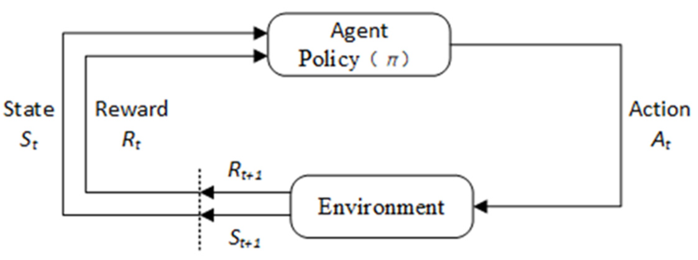
3.1. Reinforcement Learning

Reinforcement learning is an unsupervised learning process that follows a Markov decision process (MDP). Generally, finite MDPs have four parts, $\left(S,A,p,R\right)$. $S$ represents the state space of the environment, $A$ denotes the action space, $p$ represents the unknown probability of state transitions, and $R$ is the reward function. The specific process of reinforcement learning can be seen in Figure 3.

The agent interacts with the environment at each discrete moment. At each step $t$, the agent receives the environment’s state $s_t$ and selects an action $a_t$ according to the current policy $\pi$ and then receives a reward value $r_t$ from the environment to evaluate the quality of $a_t$, where $s_t\in S$, $a_t\in A$, $r_t\in R$. The decision-making process can be expressed as follows:

$$a_t=\pi \left(s_t\right)$$

(3)

The environment’s state will change to $s_{t+1}$ after the agent performs the action $a_t$, with $p\left(s_{t+1}\right|s_t,a_t)$ as the transition probability. Reinforcement learning aims to maximize the agent’s reward value to find the optimal strategy $\pi *$.

3.2. SAC Algorithm

The SAC algorithm was proposed by Haarnoja [33], which is characterized by introducing entropy regularization into the policy. The algorithm considers maximizing the sum of expected rewards and the policy entropy, which improves the explorable ability of the policy. Thus, it can converge to the optimal value more efficiently. The optimal policy $\pi *$ can be expressed as follows:

$$\pi *=arg\underset{\pi }{\mathit{max}}{\mathbb{E}}_{\left(s_t,a_t\right)~{\rho }_{\pi }}[\sum _{t}R\left(s_t,a_t\right)+\alpha H\left(\pi \right(\cdot \left|s_t\right))]$$

(4)

The SAC is a reinforcement learning algorithm based on the actor–critic structure. The actor is the policy function to generate actions that the agent uses to interact with the environment, represented by ${\pi }_{\varphi }(a_t|s_t)$. The policy update equation can be obtained by minimizing the KL divergence:

$$J_{\pi }\left(\varphi \right)={\mathbb{E}}_{s_t\sim \mathcal{D},a_t~{\pi }_{\varphi }}[log{\pi }_{\varphi }\left(a_t|s_t\right)-\frac{1}{\alpha }{Q}_{\theta }\left(s_t,a_t\right)+logZ(s_t)]$$

(5)

The critic is the value function that evaluates actions output by the actor, which guides the updating of the policy and is represented by $Q_{\theta }(s_t,a_t)$. The TD error method is used to update the value function of critic:

$$\begin{gathered} J_Q\left(\theta \right)={\mathbb{E}}_{\left(s_t,a_t,s_{t+1}\right)~\mathcal{D},a_{t+1~{\pi }_{\varphi }}}[\frac{1}{2}{(Q_{\theta }\left(s_t,a_t\right)-(r\left(s_t,a_t\right)+\gamma (Q_{\stackrel{-}{\theta }}\left(s_{t+1},a_{t+1}\right) \\ -\alpha \mathrm{l}\mathrm{o}\mathrm{g}({\pi }_{\varphi }(a_{t+1}|s_{t+1}))))}^2] \end{gathered}$$

(6)

As an off-policy algorithm, the SAC also stores the experience samples $(s_t,a_t,s_{t+1},R\left(s_t,a_t\right))$ collected by the agent in the previous episodes in the replay buffer. During training, these samples are randomly sampled to update the neural networks, which improves the sample efficiency of reinforcement learning.

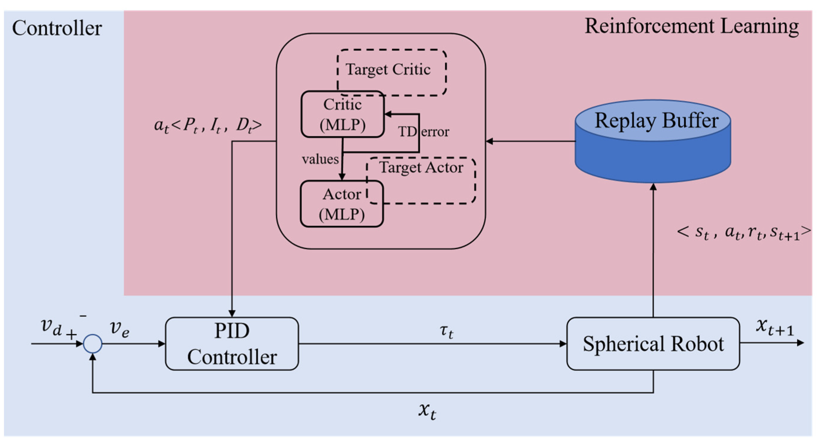
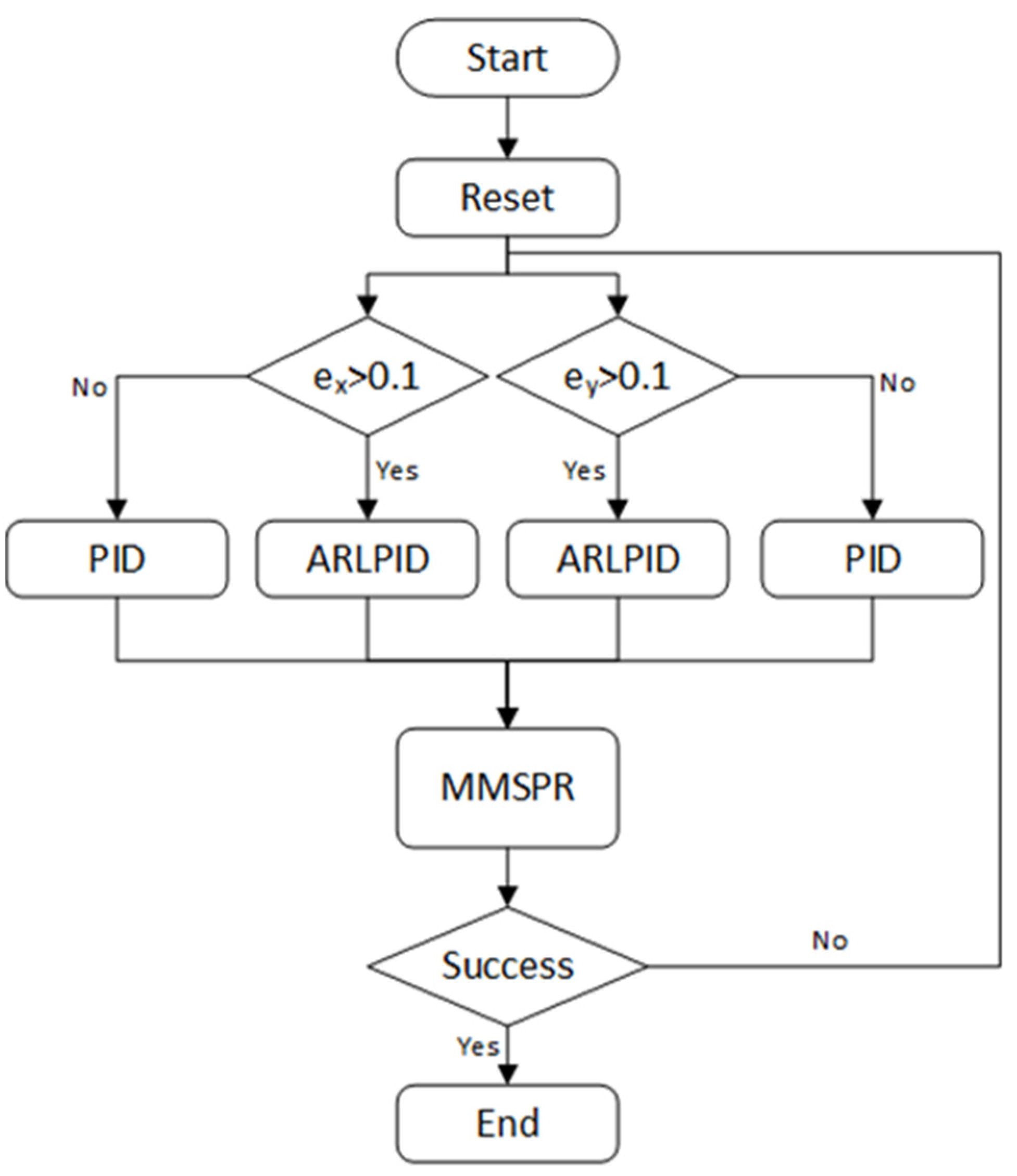
3.3. Adaptive PID Controller Based on Reinforcement Learning

The structure of the adaptive PID controller based on reinforcement learning in this paper is shown in Figure 4. It is possible to divide the entire controller into two parts. One part is the PID controller, which directly controls the motor torques of the MMSPR and realizes velocity adjustments. The other part of the controller is reinforcement learning, which outputs PID parameters for adaptive parameter adjustment.

The PID controller used in this paper is the position PID controller, whose mathematical expression can be formulated as:

$$u\left(t\right)=K_{p}e\left(t\right)+K_i\sum _{n=0}^{t}e\left(n\right)+K_d(e\left(t\right)-e\left(t-1\right))$$

(7)

For reinforcement learning, choosing appropriate state space, action space, and reward function is essential. To solve the velocity control problem, we select the dynamic characteristics of the MMSPR as observations. Specifically, the rotation angles and angular velocities of the MMSPR and the pendulum around the X and Y axes are involved. In addition, to facilitate the SAC algorithm establishing a mapping between the MMSPR’s velocity errors and the controller parameters more effectively, velocity errors of the MMSPR in X and Y directions are added into the state space, namely $e_x$, and $e_y$. As a result, the state space of reinforcement learning is ten dimensions. According to the algorithm architecture proposed in this paper, the actions of reinforcement learning are the parameters of the PID controller, as shown below:

$$a_t=\pi \left(s_t\right)=\left(K_{px}, K_{py}, K_{ix, }{K}_{iy}, K_{dx}{, K}_{dy}\right)$$

(8)

To ensure the stability of the control system, the action ranges are set to $K_{ps}=[0,3]$, $K_{is}=[0,1]$, $K_{ds}=[0,0.5]$, $s=\{x,y\}$. Furthermore, since the motor torques are limited in real-world applications, the output ranges of the PID controller are set to be within 10 Nm, ${\tau }_x,{\tau }_y\in (-10 \mathrm{N}\mathrm{m},10 \mathrm{N}\mathrm{m})$.

An important part of reinforcement learning is designing an appropriate reward function, which determines whether the agent can converge to the optimal solution. In this paper, our purpose is to control the MMSPR’s rolling velocities, that is, to reduce the errors between the actual and desired velocity of the MMSPR in X and Y directions. The velocity errors $e_x$ and $e_y$ are formulated as:

$$e_x={\dot{x}}_1\times R-v_{xd},e_y={\dot{x}}_3\times R-v_{yd}$$

(9)

where ${\dot{x}}_1$ and ${\dot{x}}_3$ are the rolling angular velocities of the MMSPR in the X and Y directions, respectively.

Therefore, the smaller $e_x$ and $e_y$ are, the larger the reward value of the agent will be. In order to obtain smaller static errors when the system is stable, $e_x$ and $e_y$ in the reward function are multiplied by a certain ratio. When the velocity errors remain large, the reward should change sharply to expedite the convergence. However, it is expected to be stable when the errors are small to ensure the agent outputs actions that maintain small errors. Therefore, tanh is used to make the 2-norm of the velocity error nonlinear, and the reward function is defined as:

$$\begin{array}{c}reward1=1-\mathit{tanh}\left(10\times \left|e_1\right|\right)\\ reward2=1-\mathit{tanh}\left(10\times \left|e_2\right|\right)\\ reward=0.5\times reward1+0.5\times reward2\end{array}$$

(10)

Due to the utilization of the tanh function, the velocity errors are difficult to reduce after it is below a threshold. Switching control is introduced into our controller to obtain smaller errors further. After the errors fall below the threshold value $\alpha$, the controller will switch from the variable-parameter PID controller adjusted by reinforcement learning to the PID controller with fixed parameters.

The threshold value $\alpha$ is set to 0.1, which means that the variable-parameter PID controller works when $e_x$ and $e_y$ are greater than 0.1. When $e_x$ and $e_y$ are less than 0.1, the controller will switch to the PID controller with fixed parameters. The logic of switching control is shown in Figure 5.

The MMSPR is considered to achieve the desired velocities successfully when $\left|e_1\right|$ and $\left|e_2\right|$ are less than 0.0001 and the reward value is larger than 0.999.

4. Simulations

4.1. Simulation Environment

In this paper, the simulation environment is built in Pycharm2022, and the computer environment is Windows 10. The CPU used is an AMD 5600X with 16 GB of RAM. The reinforcement learning algorithm is achieved with Pytorch, and its parameters are shown in

Table 1. Parameters of SAC algorithm.

Parameters	Value
Learning rate of actor	0.001
Actor network	128 × 128
Learning rate of critic	0.0005
Critic network	128 × 128
Discount ($\gamma$)	0.99
Batch size	128
Max_epoch	1000
Optimizer	Adam
Length of an episode	200 steps
Soft target update ($\tau$)	0.005
Replay_buffer_size	1,000,000

.

Since the maximum velocity of the MMSPR prototype is 0.24 m/s, the initial velocity of the MMSPR is set to a random value in the range of [0, 0.24] in the simulation environment, and the desired velocity $v_d$ is set to 0 m/s. We aim to train a controller that enables the MMSPR with different initial postures and velocities to brake rapidly. In the simulation process, the sampling time is 0.005 s, and the total simulation time is 1 s, timestep = 200. The related parameters of the MMSPR are shown in

Table 2. Parameters of the MMSPR.

Parameters	Value
M, the mass of shell	0.2 kg
m, the mass of pendulum	0.6 m
R, the radius of sphere	0.08 m
L, the length of swing arm	0.023 m
g, the acceleration of gravity	9.81 m/s2

.

Considering the uncertain interference caused by the inaccurate dynamic model, sensor noise, and environmental noise, a 5% model error and 2% measurement error were added to the MMSPR’s mass and the observed state values in the training and testing environment. Additionally, pulse interferences with values of 0.08, 0.04, 0.08, and 0.04 were added to ${\dot{x}}_1$, ${\dot{x}}_2$, ${\dot{x}}_3$, and ${\dot{x}}_4$ at 0.1s to simulate collision scenarios.

4.2. Simulation Results and Analysis

We argue that our algorithm’s performance improvement depends on three pivotal factors: the hierarchical control structure, the switching control strategy, and adjustable controller parameters. To substantiate the significance of these factors in the design method, this section conducts a comparative analysis across two scenarios: the spherical robot’s motion stability and rapid braking. We provide the abbreviation of each method: the adaptive PID control method based on reinforcement learning with switching control (ARLPID), fixed-parameter PID control method (PID), pure reinforcement learning control method that directly outputs motor torque (Torque_RL), and adaptive PID control method based on reinforcement learning without switching control (RLPID).

This section initially presents the average reward curves during the training process for ARLPID, RLPID, and Torque_RL (Figure 6). Noting that the concept of average reward applies solely to reinforcement learning methods, PID is not encompassed in this comparison.

The average reward value of ARLPID is higher than that of RLPID, and the fluctuation of reward value is slighter after the algorithm converges. However, the average reward curve of Torque_RL fluctuates sharply and finally remains at a lower value.

The success rate of different algorithms in the test environment is presented in

Table 3. Test success rate of different algorithms.

Algorithms	Success Rate
ARLPID (ours)	100%
Torque_RL	0%
RLPID	91%

. As shown in the table, both ARLPID and PID can successfully realize the braking of the MMSPR with a 100% success rate in the case of random initial velocities and various interferences. In comparison, RLPID only has a 91% success rate. In contrast, the success rate of Torque_RL is 0%, which shows that it cannot solve the velocity control problem of the MMSPR after training.

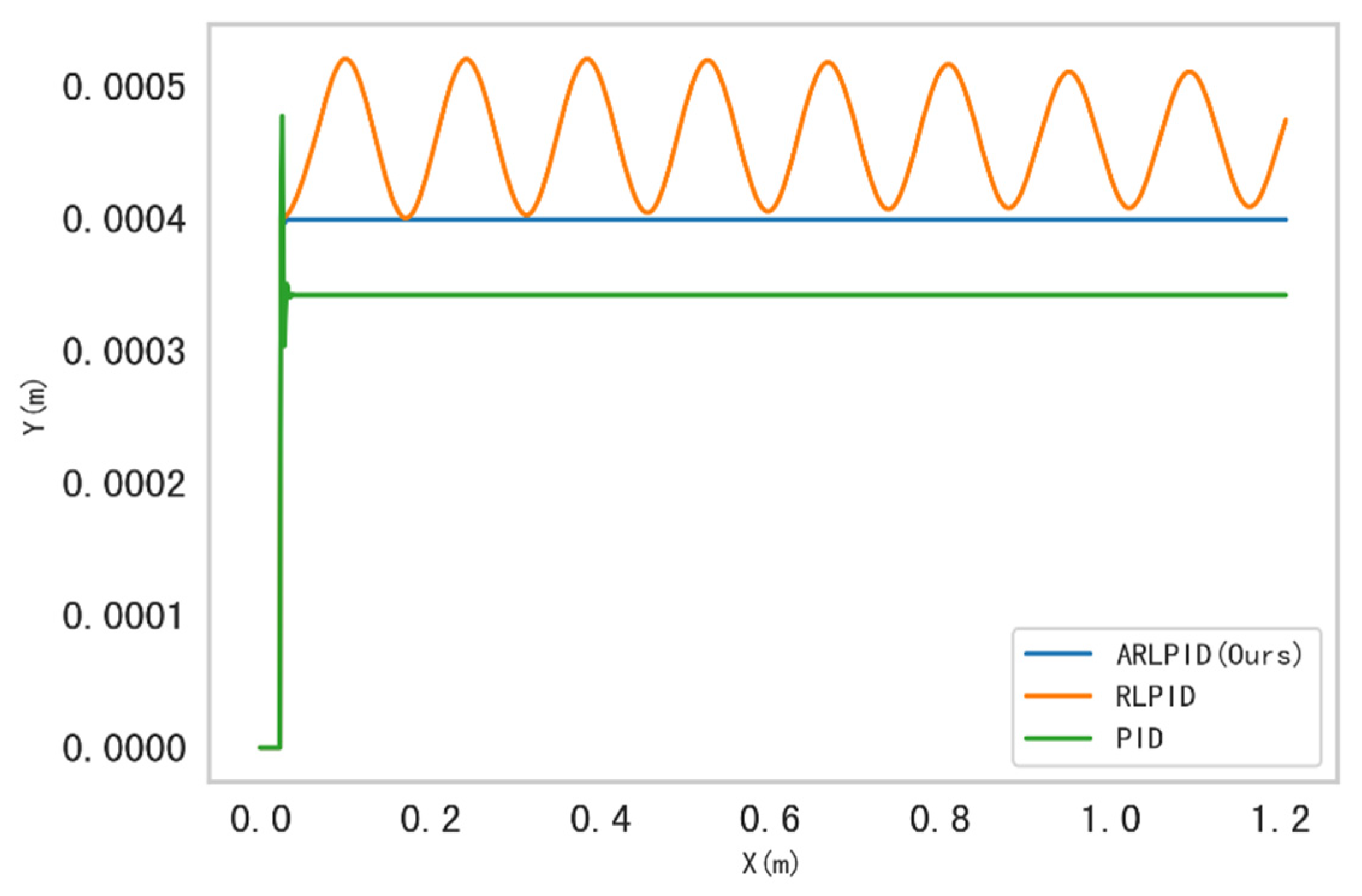
4.2.1. Motion Stability

To verify the effectiveness of our method in maintaining the robot’s motion stability, in this section, we simulate a scenario of an MMSPR moving straightly on a flat surface. We apply disturbances in the turning direction to simulate posture disturbances resulting from structural errors, non-uniform mass distribution, and collisions.

The robot’s desired speed in the turning direction is established as: $v_{yd}$ = 0 m/s. The simulation duration is 5 s, and the results are shown in Figure 7 and Figure 8.

Figure 7 shows the speed changes in the turning direction of the MMSPR under different control methods. By adjusting the controller parameters, ARLPID reduces the overshoot by approximately 93% compared to PID with fixed parameters, costing a shorter convergence time. It takes only 0.02 s to converge, compared to 0.03 s required by PID. RLPID performs the best in convergence speed, requiring just 0.01 s, which is faster than PID, and its overshoot is also lower than PID. However, there is a small fluctuation of 0.06% in the robot’s speed after convergence, and it does not stabilize completely. This might be attributable to using the tanh function when designing the reward function of reinforcement learning. The reward value tends to saturate and stabilize when the error is small. Hence, it cannot continue to optimize. This also results in a lower success rate of RLPID in the testing environment. In comparison, ARLPID introduces a switching control strategy to eliminate static errors, which can avert speed fluctuations prominently.

Figure 8 displays the robot’s trajectory during the simulation process. The maximum offset displacement of the robot reaches 0.00048 m under the control of PID. With RLPID control, the trajectory significantly fluctuates and cannot maintain stability, showing a maximum offset displacement of 0.00052 m. However, due to variable parameters and switching control strategy, the trajectory under ARLPID control changes smoothly, with the minimum offset displacement being merely 0.00041 m.

The simulation results show that the ARLPID method, which introduces variable controller parameters and the switching control strategy, significantly enhances control performance in the problem of the spherical robot’s motion stability. This improvement is especially notable compared to the traditional PID with fixed parameters and the RLPID method, which lacks the switching control strategy.

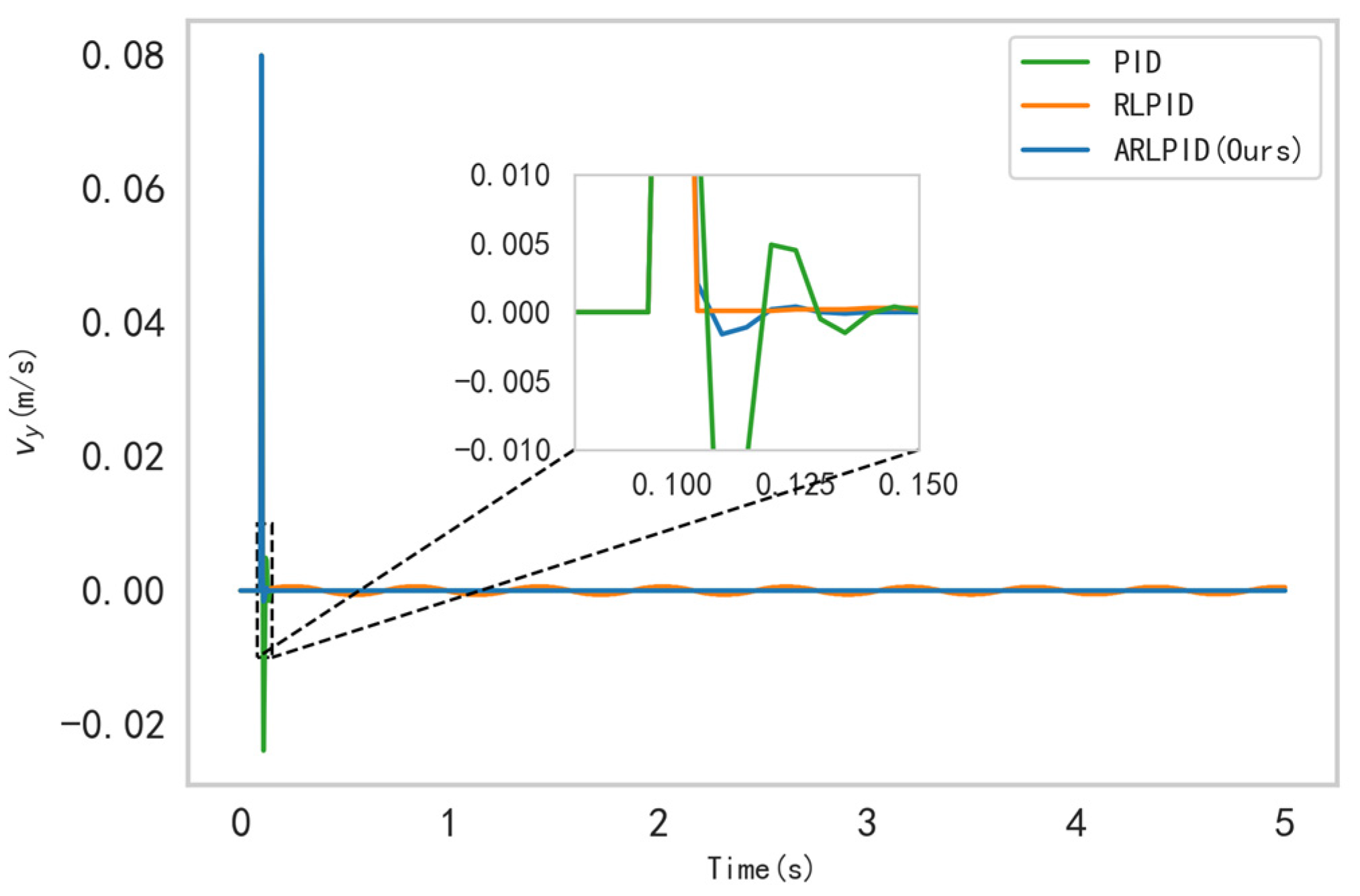
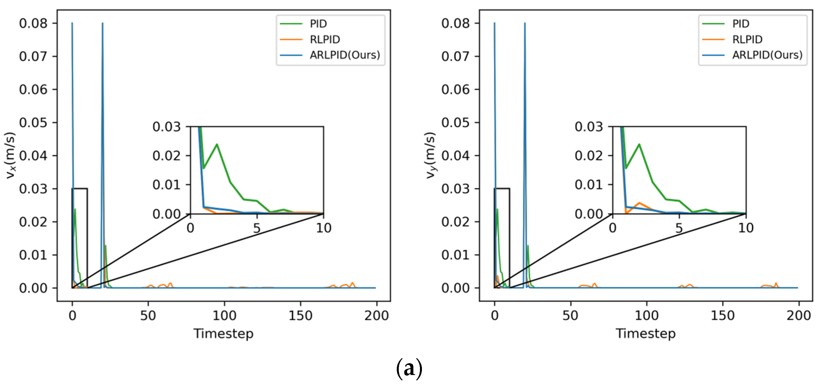
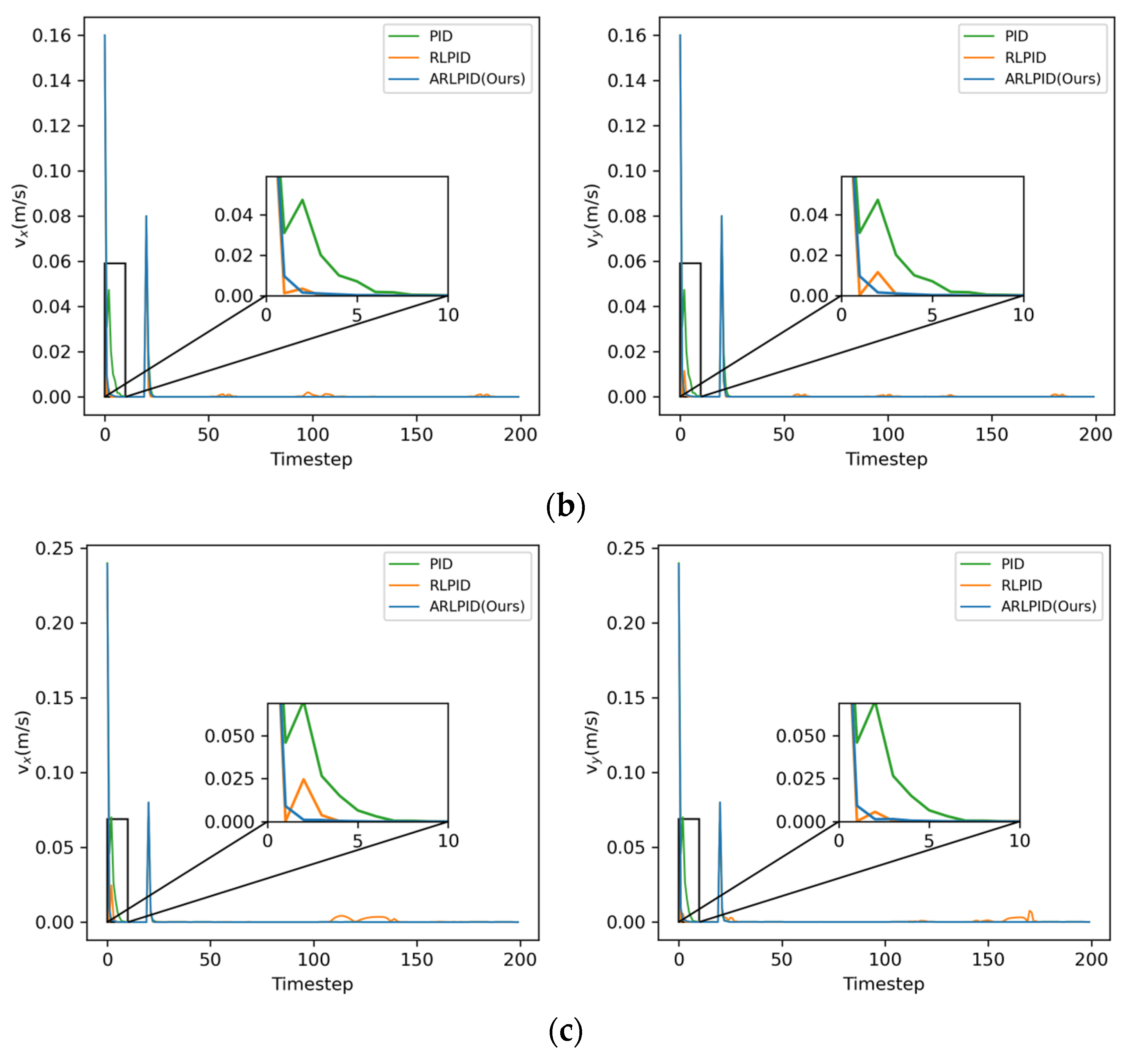
4.2.2. Rapidly Brake

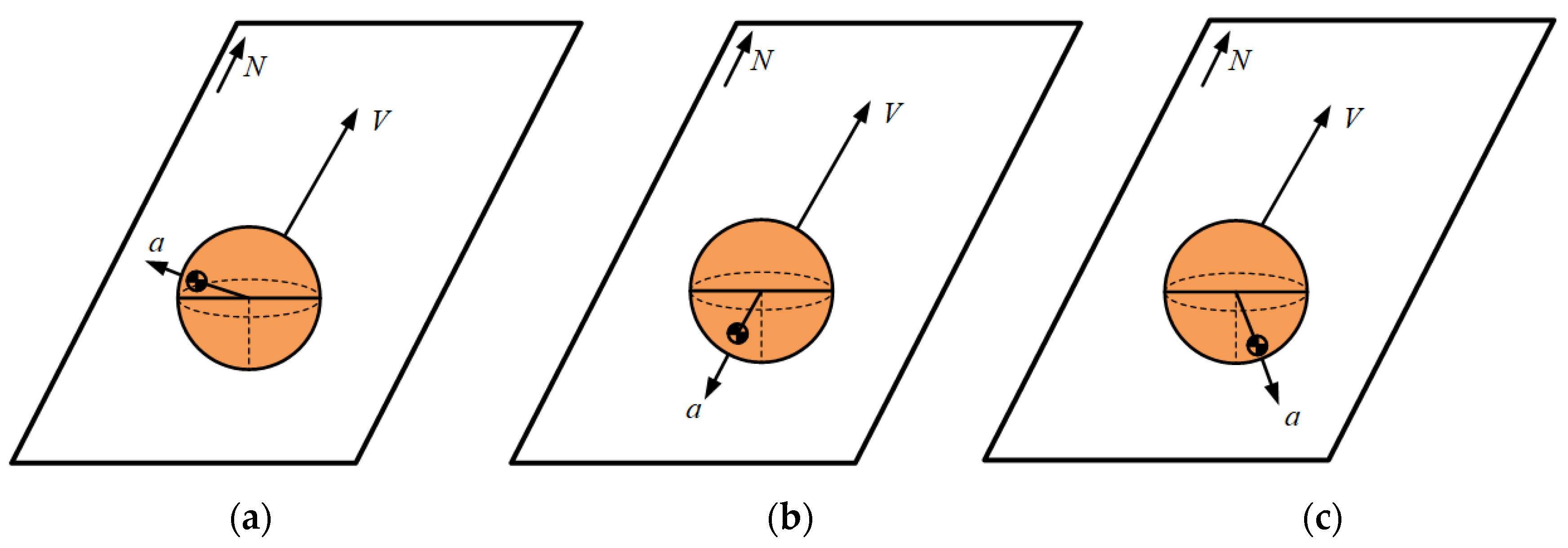
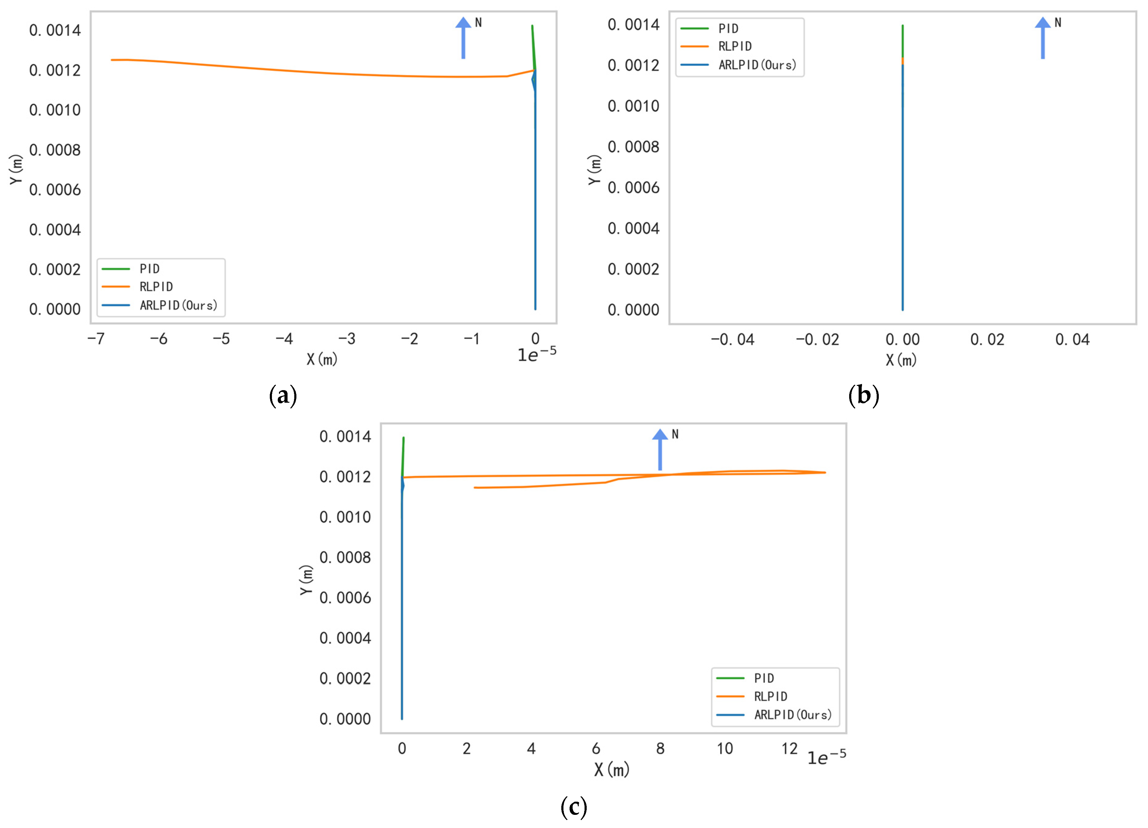
In this section, we simulated the task of MMSPR rapid braking after landing. To provide a more detailed description of the robot’s state after its landing, we will simulate the different postures and velocities of the MMSPR after landing, respectively.

Postures

Three distinct initial states of the robot are set to simulate its various random postures after landing fully. In these states, the robot’s directions are consistent with the forward movement direction (north) but with acceleration in different directions: northwest, north, and northeast (as shown in Figure 9). These three acceleration directions represent that the robot may deviate in different directions after landing, providing a more comprehensive scenario for algorithm validation.

In the first scenario, related parameters are set as: $v_{x1}=0.24 \mathrm{m}/\mathrm{s}$, $v_{y1}=0 \mathrm{m}/\mathrm{s}$, ${\alpha }_1=0.1 \mathrm{r}\mathrm{a}\mathrm{d}$, ${\beta }_1=0.2 \mathrm{r}\mathrm{a}\mathrm{d}$, and the remaining parameters are zero. In the second scenario, parameters are set as: $v_{x2}=0.24 \mathrm{m}/\mathrm{s}$, $v_{y2}=0.24 \mathrm{m}/\mathrm{s}$, ${\alpha }_2=0.1 \mathrm{r}\mathrm{a}\mathrm{d}$, ${\beta }_2=-0.2 \mathrm{r}\mathrm{a}\mathrm{d}$, and the remaining parameters are zero. In the third scenario, parameters are set as: $v_{x3}=0 \mathrm{m}/\mathrm{s}$, $v_{y3}=0.24 \mathrm{m}/\mathrm{s}$, ${\alpha }_3=-0.1 \mathrm{r}\mathrm{a}\mathrm{d}$, ${\beta }_3=-0.2 \mathrm{r}\mathrm{a}\mathrm{d}$, and the remaining parameters are zero. The desired values for the speed of the MMSPR are set as: $v_{xd}=v_{yd}=0 \mathrm{m}/\mathrm{s}$. The results of each control method under different states are shown in Figure 10 and Figure 11.

To more intuitively compare the effects of various control methods, this section will mainly analyze the simulation results of the first scenario. As seen in Figure 10a, there is a substantial overshoot during the convergence with PID. The convergence time of $v_x$ and $v_y$ is 0.04 s and 0.01 s, respectively, which are slower than the ARLPID and RLPID methods using variable parameters. With RLPID, the speed error converges more rapidly, requiring only 0.01 s for both $v_x$ and $v_y$ to converge. However, the robot’s speed fluctuates significantly when disturbances occur. Under SMC, the robot’s speed changes relatively smoothly, but it has the longest convergence time, with $v_x$ and $v_y$ taking 1.04 s and 0.535 s, respectively. Additionally, there is a periodic speed fluctuation during the convergence. Compared with the above methods, the overshoot under ARLPID is reduced by about 81% compared to the PID method, eliminating the speed fluctuation observed in RLPID. This method allows $v_x$ and $v_y$ to converge quickly within 0.03 s and 0.01 s, respectively, and shows strong resistance to disturbances. The convergence times for other scenarios are shown in

Table 4. The braking time of robot speed.

Scenarios	Velocity	PID	RLPID	ARLPID
The first scenario	$v_x$	0.04 s	0.01 s	0.03 s
	$v_y$	0.01 s	0.01 s	0.01 s
The second scenario	$v_x$	0.035 s	0.01 s	0.025 s
	$v_y$	0.00 s	0.00 s	0.00 s
The third scenario	$v_x$	0.035 s	0.01 s	0.025 s
	$v_y$	0.01 s	0.08 s	0.01 s

.

Figure 11 shows the trajectories of different control methods during braking under different scenarios. In the first scenario, the braking displacement of the robot under PID is longer, with 0.0021 m, compared to that of RLPID and ARLPID, both of which employ variable parameters. The braking displacement under RLPID is 0.0013 m. However, the robot’s speed is not completely stable when suffering disturbances from the external environment, resulting in substantial fluctuation in its movement trajectory. The robot’s trajectory under ARLPID alters relatively smoothly, with a braking displacement of 0.0013 m, the smallest of the three methods. In the second scenario, the braking displacements of the three methods are 0.0019 m, 0.0014 m, and 0.0013 m, respectively. Similarly, in the third scenario, the braking displacements are 0.0019 m, 0.0015 m, and 0.0013 m, respectively.

Velocities

The results of the MMSPR with different initial velocities and different controllers are shown in Figure 12. As Torqu_RL cannot solve the control problem, only the results of the other three algorithms are displayed. As shown in Figure 12, although the velocity errors finally converge successfully with PID, there are obvious jitters during the error reduction, and the convergence time is longer than ARLPID. RLPID is the algorithm with the shortest convergence time, but small error fluctuations occur in the follow-up timesteps, which cannot be completely stable. The reason may be that the tanh function is used in the reward function. When the error is small, the reward function tends to be saturated and stable, so it cannot continue to guide the policy update.

With ARLPID proposed in this paper, the velocity errors converge rapidly and remain stable, which outperforms other controllers. The error convergence time of each algorithm is shown in

Table 5. The convergence time of each algorithm.

Initial Velocity	Error	PID	RLPID	ARLPID
0.08 m/s	$e_x$	0.065 s	0.065 s	0.045 s
	$e_y$	0.065 s	0.025 s	0.045 s
0.16 m/s	$e_x$	0.06 s	0.02 s	0.04 s
	$e_y$	0.06 s	0.03 s	0.04 s
0.24 m/s	$e_x$	0.055 s	0.03 s	0.045 s
	$e_y$	0.055 s	0.035 s	0.045 s

.

In summary, ARLPID performs best in maintaining motion stability and achieving rapid braking among the three control methods. It has a fast convergence speed, a small displacement offset, and stable control performance. This method can solve the problems of motion stability during the rolling and rapid braking after jumping to avoid obstacles, relying on its high adaptability and robustness.

5. Conclusions

This paper presents an adaptive PID controller based on reinforcement learning to address the motion stability of MMSPR during rolling and its rapid braking after jumping to avoid obstacles. This controller adopts the SAC algorithm for adaptively tuning the parameters of the PID controller and introduces a switching control strategy to reduce the system’s static errors.

The adaptive PID control method based on reinforcement learning proposed in this paper outperforms baseline algorithms in optimality and robustness. It ensures the motion stability of the MMSPR during its rolling process and facilitates rapid braking after crossing obstacles to avoid it reentering obstacles. Regarding motion stability, ARLPID facilitates the robot’s convergence within 0.02 s. Furthermore, this controller significantly reduces the overshoot observed in PID and eliminates the static errors in RLPID. In cases with the robot having random landing postures, ARLPID ensures the robot’s braking within 0.0013 m, which is about 38% better than PID. Furthermore, it has strong robustness and eliminates oscillation in RLPID. Under conditions with random landing speed, the simulation results show that ARLPID enables the MMSPR to brake rapidly when its initial velocity ranges from 0 to 0.24 m/s after landing. It attains a success rate of 100% and a braking time of less than 0.045 s, which is 20% faster than PID. In addition, ARLPID maintains better stability than RLPID considering external interference and collisions that might occur in the practical application.

In future work, we will further study the performance of this control method on the prototype of MMSPR. Furthermore, we will modify and optimize our control algorithm according to the experimental results.

References

1. Sagsoz, I.H.; Eray, T. Design and Kinematics of Mechanically Coupled Two Identical Spherical Robots. J. Intell. Robot. Syst. 2023, 108, 12. [Google Scholar] [CrossRef]
2. Li, M.; Sun, H.; Ma, L.; Gao, P.; Huo, D.; Wang, Z.; Sun, P. Special spherical mobile robot for planetary surface exploration: A review. Int. J. Adv. Robot. Syst. 2023, 20. [Google Scholar] [CrossRef]
3. Chi, X.; Zhan, Q. Design and modelling of an amphibious spherical robot attached with assistant fins. Appl. Sci. 2021, 11, 3739. [Google Scholar] [CrossRef]
4. Shi, L.; Zhang, Z.; Li, Z.; Guo, S.; Pan, S.; Bao, P.; Duan, L. Design, Implementation and Control of an Amphibious Spherical Robot. J. Bionic Eng. 2022, 19, 1736–1757. [Google Scholar] [CrossRef]
5. Rangapur, I.; Prasad, B.K.S.; Suresh, R. Design and Development of Spherical Spy Robot for Surveillance Operation. Procedia Comput. Sci. 2020, 171, 1212–1220. [Google Scholar] [CrossRef]
6. Michaud, F.O.; Caron, S. Roball, the Rolling Robot. Auton. Robot. 2002, 12, 211–222. [Google Scholar] [CrossRef]
7. Azizi, M.R.; Naderi, D. Dynamic modeling and trajectory planning for a mobile spherical robot with a 3Dof inner mechanism. Mech. Mach. Theory 2013, 64, 251–261. [Google Scholar] [CrossRef]
8. Borisov, A.V.; Kilin, A.A.; Mamaev, I.S. An omni-wheel vehicle on a plane and a sphere. Nelin. Dinam. 2011, 7, 785–801. [Google Scholar] [CrossRef] [Green Version]
9. Moazami, S.; Palanki, S.; Zargarzadeh, H. Design, Modeling, and Control of Norma: A Slider & Pendulum-Driven Spherical Robot. arXiv 2020, arXiv:1908.02243. [Google Scholar]
10. Wu, H.; Li, B.; Wang, F.; Luo, B.; Jiao, Z.; Yu, Y.; Wang, P. Design and Analysis of the Rolling and Jumping Compound Motion Robot. Appl. Sci. 2021, 11, 10667. [Google Scholar] [CrossRef]
11. Wang, F.; Li, C.; Niu, S.; Wang, P.; Wu, H.; Li, B. Design and Analysis of a Spherical Robot with Rolling and Jumping Modes for Deep Space Exploration. Machines 2022, 10, 126. [Google Scholar] [CrossRef]
12. Hu, Y.; Wei, Y.; Liu, M. Design and performance evaluation of a spherical robot assisted by high-speed rotating flywheels for self-stabilization and obstacle surmounting. J. Mech. Robot. 2021, 13, 061001. [Google Scholar] [CrossRef]
13. Chang, W.-J.; Chang, C.-L.; Ho, J.-H.; Lin, P.-C. Design and implementation of a novel spherical robot with rolling and leaping capability. Mech. Mach. Theory 2022, 171, 104747. [Google Scholar] [CrossRef]
14. Chen, S.-B.; Beigi, A.; Yousefpour, A.; Rajaee, F.; Jahanshahi, H.; Bekiros, S.; Martinez, R.A.; Chu, Y. Recurrent Neural Network-Based Robust Nonsingular Sliding Mode Control With Input Saturation for a Non-Holonomic Spherical Robot. IEEE Access 2020, 8, 188441–188453. [Google Scholar] [CrossRef]
15. Fortuna, L.; Frasca, M.; Buscarino, A. Optimal and Robust Control: Advanced Topics with MATLAB®; CRC Press: Boca Raton, FL, USA, 2021. [Google Scholar]
16. Zhou, T.; Xu, Y.-G.; Wu, B. Smooth Fractional Order Sliding Mode Controller for Spherical Robots with Input Saturation. Appl. Sci. 2020, 10, 2117. [Google Scholar] [CrossRef] [Green Version]
17. Ma, W.; Chang, C.; Cao, Y.; Wang, F.; Wang, P.; Li, B. Attitude control of multi-motion mode spherical probe robots based on decoupled dynamics. In Proceedings of the Advances in Guidance, Navigation and Control; Yan, L., Duan, H., Deng, Y., Eds.; Springer Nature: Singapore, 2023; pp. 5850–5861. [Google Scholar]
18. Ma, L.; Sun, H.; Song, J. Fractional-order adaptive integral hierarchical sliding mode control method for high-speed linear motion of spherical robot. IEEE Access 2020, 8, 66243–66256. [Google Scholar] [CrossRef]
19. Shi, L.; Hu, Y.; Su, S.; Guo, S.; Xing, H.; Hou, X.; Liu, Y.; Chen, Z.; Li, Z.; Xia, D. A Fuzzy PID Algorithm for a Novel Miniature Spherical Robots with Three-dimensional Underwater Motion Control. J. Bionic Eng. 2020, 17, 959–969. [Google Scholar] [CrossRef]
20. Guo, J.; Li, C.; Guo, S. A novel step optimal path planning algorithm for the spherical mobile robot based on fuzzy control. IEEE Access 2020, 8, 1394–1405. [Google Scholar] [CrossRef]
21. Guo, J.; Li, C.; Guo, S. Path optimization method for the spherical underwater robot in unknown environment. J. Bionic Eng. 2020, 17, 944–958. [Google Scholar] [CrossRef]
22. Liu, Y.; Wang, Y.; Guan, X.; Wang, Y.; Jin, S.; Hu, T.; Ren, W.; Hao, J.; Zhang, J.; Li, G. Multi-terrain velocity control of the spherical robot by online obtaining the uncertainties in the dynamics. IEEE Robot. Autom. Lett. 2022, 7, 2732–2739. [Google Scholar] [CrossRef]
23. Liu, Y.; Wang, Y.; Guan, X.; Hu, T.; Zhang, Z.; Jin, S.; Wang, Y.; Hao, J.; Li, G. Direction and trajectory tracking control for nonholonomic spherical robot by combining sliding mode controller and model prediction controller. IEEE Robot. Autom. Lett. 2022, 7, 11617–11624. [Google Scholar] [CrossRef]
24. Kayacan, E.; Bayraktaroglu, Z.Y.; Saeys, W. Modeling and control of a spherical rolling robot: A decoupled dynamics approach. Robotica 2012, 30, 671–680. [Google Scholar] [CrossRef] [Green Version]
25. Kamis, N.N.; Embong, A.H.; Ahmad, S. Modelling and Simulation Analysis of Rolling Motion of Spherical Robot. IOP Conf. Ser. Mater. Sci. Eng. 2017, 260, 012014. [Google Scholar] [CrossRef] [Green Version]
26. Zhang, L.; Ren, X.; Guo, Q. Balance and velocity control of a novel spherical robot with structural asymmetry. Int. J. Syst. Sci. 2021, 52, 3556–3568. [Google Scholar] [CrossRef]
27. Qin, Y.; Zhang, W.; Shi, J.; Liu, J. Improve PID controller through reinforcement learning. In Proceedings of the 2018 IEEE CSAA Guidance, Navigation and Control Conference (CGNCC), Xiamen, China, 10–12 August 2018; pp. 1–6. [Google Scholar]
28. Sutton, R.S.; Barto, A.G. Reinforcement Learning: An Introduction; MIT Press: Cambridge, MA, USA, 2018. [Google Scholar]
29. Zheng, Q.; Tang, R.; Gou, S.; Zhang, W. A PID Gain Adjustment Scheme Based on Reinforcement Learning Algorithm for a Quadrotor. In Proceedings of the 2020 39th Chinese Control Conference (CCC), Shenyang, China, 27–29 July 2020; pp. 6756–6761. [Google Scholar]
30. Wang, S.; Yin, X.; Li, P.; Zhang, M.; Wang, X. Trajectory Tracking Control for Mobile Robots Using Reinforcement Learning and PID. Iran. J. Sci. Technol. Trans. Electr. Eng. 2020, 44, 1059–1068. [Google Scholar] [CrossRef]
31. Guan, Z.; Yamamoto, T. Design of a Reinforcement Learning PID Controller. IEEJ Trans. Elec. Electron. Eng. 2021, 16, 1354–1360. [Google Scholar] [CrossRef]
32. Park, J.; Kim, H.; Hwang, K.; Lim, S. Deep Reinforcement Learning Based Dynamic Proportional-Integral (PI) Gain Auto-Tuning Method for a Robot Driver System. IEEE Access 2022, 10, 31043–31057. [Google Scholar] [CrossRef]
33. Haarnoja, T.; Zhou, A.; Abbeel, P.; Levine, S. Soft Actor-Critic: Off-Policy Maximum Entropy Deep Reinforcement Learning with a Stochastic Actor. arXiv 2018, arXiv:1801.01290. [Google Scholar]
Figure 1. The structure schematic of the MMSPR: (a) structural diagram of MMSPR; (b) simplified model of MMSPR.
Applsci 13 08218 g001
Figure 2. Establishment of spherical robot coordinate system: (a) spatial coordinate system of spherical robot; (b) projection of coordinate system on Y A Z A plane; (c) projection of coordinate system on X A Z A plane.
Applsci 13 08218 g002
Figure 3. The specific process of reinforcement learning.
Applsci 13 08218 g003
Figure 4. The structure of the designed controller. The red part represents the reinforcement learning module, which adjusts the parameters of the PID controller. The blue part represents the controller module, which outputs the motor torques.
Applsci 13 08218 g004
Figure 5. The logic of switching control.
Applsci 13 08218 g005
Figure 6. The mean reward curve in the training process of different algorithms.
Applsci 13 08218 g006
Figure 7. Control effects of different control methods.
Applsci 13 08218 g007
Figure 8. Trajectory of different control methods.
Applsci 13 08218 g008
Figure 9. Three initial scenarios of MMSPR after landing: (a) the first scenario; (b) the second scenario; (c) the third scenario.
Applsci 13 08218 g009
Figure 10. Velocity variation of MMSPR under different scenarios: (a) the change in velocity in the first scenario (with external interference); (b) the change in velocity in the second scenario (with external interference); (c) the change in velocity in the third scenario (with external interference).
Applsci 13 08218 g010aApplsci 13 08218 g010b
Figure 11. Brake trajectory of MMSPR under different control methods: (a) the change in trajectory in the first scenario; (b) the change in trajectory in the second scenario; (c) the change in trajectory in the third scenario.
Applsci 13 08218 g011
Figure 12. The results of different controllers: (a) initial speed is 0.08 m/s; (b) initial speed is 0.16 m/s; (c) initial speed is 0.24 m/s.
Applsci 13 08218 g012aApplsci 13 08218 g012b