Peripheral Pulmonary Lesions Classification Using Endobronchial Ultrasonography Images Based on Bagging Ensemble Learning and Down-Sampling Technique

Abstract

Lung cancer is the second most common cancer in the world, with an average five-year survival rate of 15 percent. Approximately 238,340 people were diagnosed in the US in 2023 based on the estimation of the American Cancer Society, and 127,070 people died from it. Cancer has always been a big problem for scientists. There has never been a good solution. So, the early detection of cancer is particularly important. In recent years, endobronchial ultrasonography (EBUS) images have been used more and more in the diagnosis of lung cancer because of their advantages of good real-time performance, no radiation, and superior performance. This research aims to develop a computer-aided diagnosis (CAD) system to differentiate benign and malignant peripheral pulmonary lesions (PPLs). The efficacy of this framework was evaluated on a dataset comprising 69 cases of lung carcinoma, encompassing 59 malignant instances and 10 benign cases. The final experimental results of accuracy, F1-Score, AUC, PPV, NPV, sensitivity, and specificity were 0.7, 0.63, 0.75, 0.84, 0.68, 0.56, and 0.85, respectively. From the experiment results, the developed CAD system has the potential ability to diagnose PPLs by using the EBUS images based on Deep Learning.

1. Introduction

In accordance with GLOBOCAN 2020 data, which encompasses cancer incidence and mortality estimates compiled by the International Agency for Research on Cancer, the global tally for new cancer cases in 2020 amounted to approximately 19.3 million, with a corresponding death toll of 10.0 million (excluding nonmelanoma skin cancer, the figures stand at 18.1 million new cases and 9.9 million deaths). Among these cases, lung cancer held the second position in terms of incidence, accounting for 11.4% of all reported new cases. However, it claimed the highest number of lives, accounting for 18% of the total deaths [1]. Lung cancer remains the utmost proponent of cancer death worldwide, with a mere 15% overall five-year survival rate. Most cases are diagnosed at an advanced stage when treatment outcomes are not ideal and newly diagnosed patients develop locally advanced or metastatic diseases [2]. Thus, early diagnosis is imperative for propelling lung cancer survival rates, successful treatment, and management. Unfortunately, early lung cancer detection methods are currently insufficient.

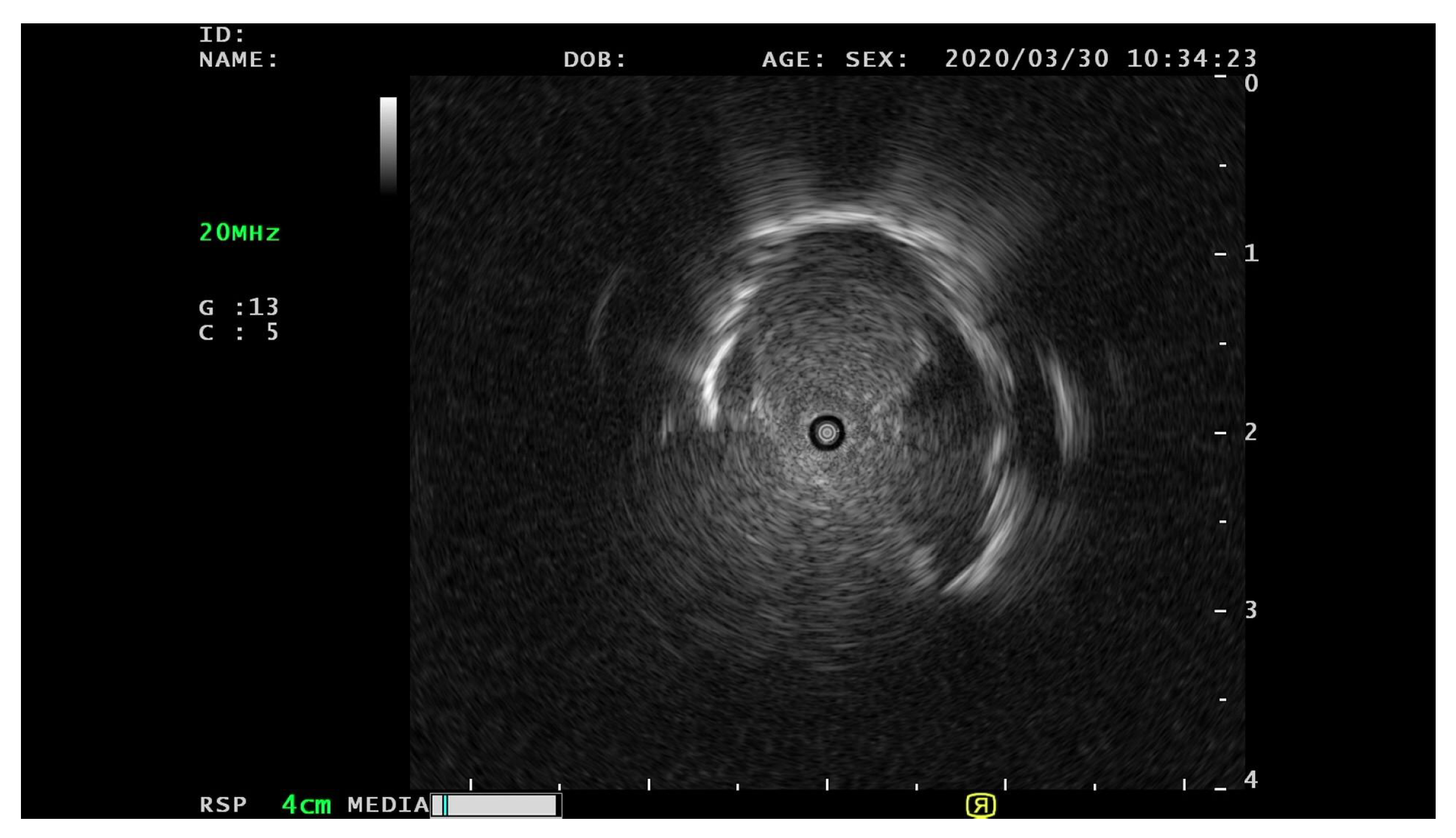
A thoracic radiograph (TR), commonly known as a chest X-ray (CXR), serves as the primary modality employed in the initial assessment of individuals with suspected lung malignancy. Its widespread accessibility, technical feasibility, minimal risk, and cost-effectiveness contribute to its frequent utilization in this context. The biopsy is another prominent clinical method for lung cancer diagnosis, but taking a biopsy from peripheral pulmonary nodules is notably challenging for physicians. Although computed tomography (CT)-guided percutaneous biopsies are often preferred, pneumothorax, bleeding, and other procedure complications are sometimes problematic. Transbronchial biopsy is customary in Japan, with several steps to ensure a high diagnostic yield: (1) accurately reach the target, (2) confirm the target lesion, (3) collect the biopsy sample from the target, and (4) adequate sampling from the target. In addition, rEBUS technology aids in confirming that the device has reached the target. However, a successful sampling is not always guaranteed because rEBUS is not a real-time guided biopsy procedure. Nonetheless, rEBUS’s image analysis will facilitate additional sampling during the biopsy procedure and treatment recommendations.

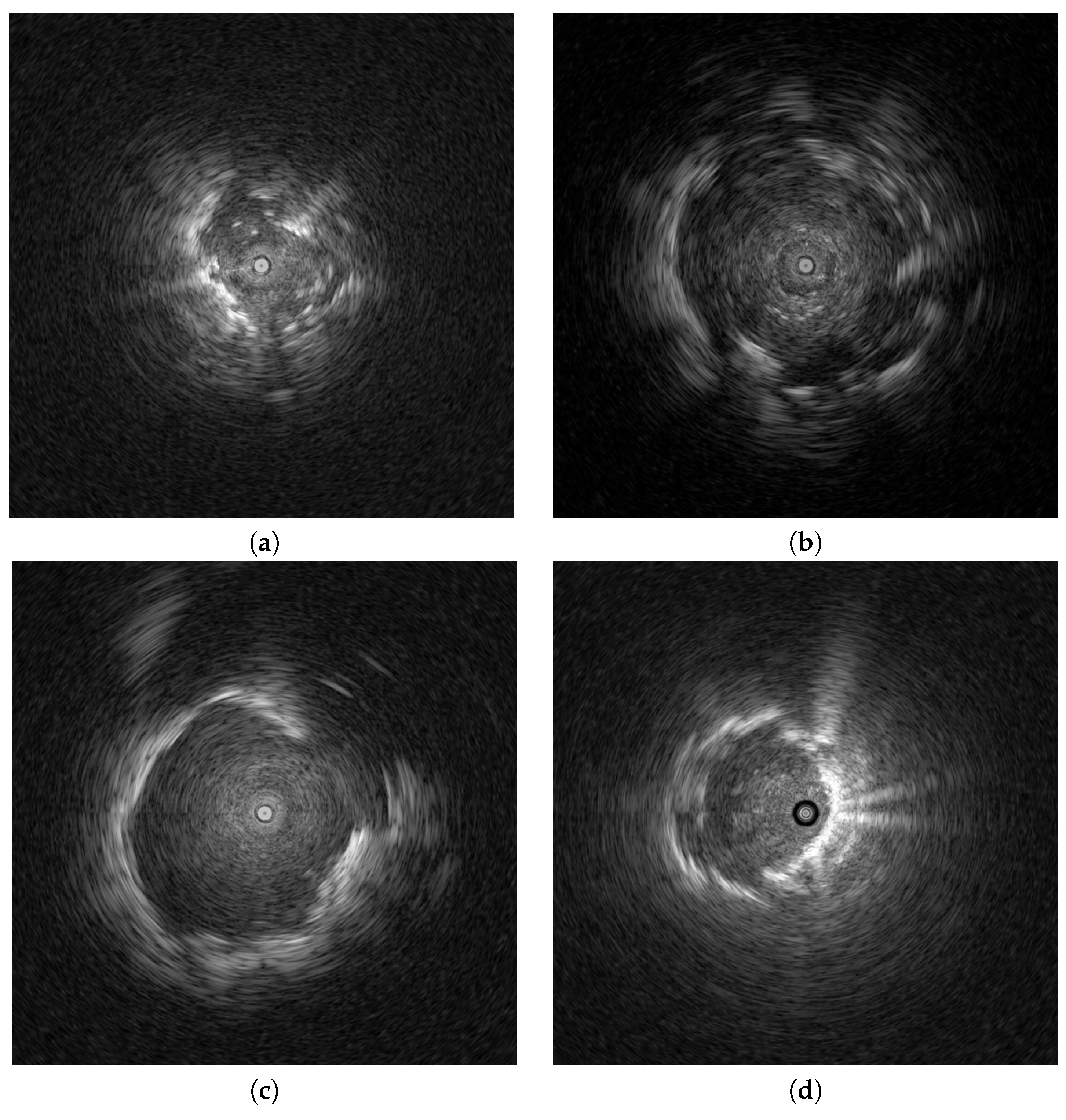
Endobronchial ultrasonography (EBUS) has recently been used to screen for peripheral pulmonary lesions. This radiation-free medical technique uses ultrasound and real-time scanning to diagnose and stage lung diseases, incorporating an endoscope to access the lungs through the airways. It provides high-resolution images for real-time lung tissue and surrounding structure visualizations. EBUS is routinely employed for lung nodule evaluations, lung cancer staging, and various lung disease diagnoses, enabling physicians to make informed decisions regarding treatment options. Clinical studies have attempted to distinguish peripheral pulmonary lesions (PPLs) from EBUS images [3,4,5,6]; however, benign and malignant PPL distinctions are subjective to physician experience and vex even the most experienced physicians. With current artificial intelligence (AI) advancements, AI technology has been increasingly integrated into the medical field. Many computer-aided diagnoses (CAD) have been presented to assist physicians through medical image processing.

Khomkham et al. [3] employed two radiomics features, namely the adaptive weighted sum of the upper triangular gray-level co-occurrence matrix (GLCM) and the adaptive weighted sum of the lower triangular GLCM, to visualize the classifications of peripheral pulmonary lesions using EBUS images. The classification of these lesions was performed using the genetic algorithm in conjunction with a support vector machine (SVM) [7] approach. Within the following year, a three-branch classification framework was proposed for differentiating PPLs. The radiomics feature and patient data are used in Branch 1 to train the random forest classifier [8]. In Branch 2, convolutional neural network (CNN)-based models are prepared with EBUS images. Lastly, multi-patch EBUS images are selected from the original EBUS images to train the multi-patch-based model in Branch 3. Thus, three models are aggregated using the weighted ensemble strategy. Chen et al. 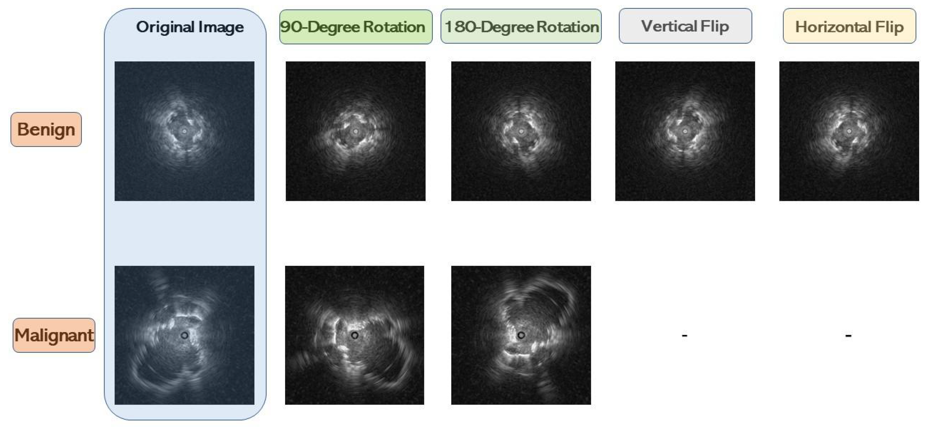[4] proposed a CAD system that automatically differentiates benign and malignant PPLs for early lung cancer detection with EBUS images. Notably, this CAD system incorporates the transformer learning technique, and rotation and flipping augmentation methods are also included in the training dataset to avoid overfitting. CNN models extract features, which the SVM then classifies.

Jinsa et al. [9] also designed a computer-aided classification method to differentiate lung cancer using CT images from an artificial neural network (ANN). Statistical parameters, such as mean, standard deviation, skewness, kurtosis, fifth central moment, and sixth central moment, are used for classification. Alakwaa et al. [10] introduced a CAD system for lung cancer classification utilizing CT scans and a dataset from the 2017 Kaggle Data Science Bowl. In this two-stage system, a three-dimensional convolutional neural network (3D-CNN) classifies CT scans as lung cancer positive or negative. First, the modified U-Net detects nodule candidates in CT images of segmented lungs. Then, the regions where most nodule candidates are likely located are fed into a 3D-CNN to provide a final classification result. Alternatively, Chaunzwa et al. [11] employed a radiomics methodology to predict the histology of non-small cell lung cancer tumors using standard-of-care computed tomography (CT) data.

Moreover, a comparable discriminative performance yielded reliable results by implementing machine learning classifiers such as k-nearest neighbor and SVM for CNN-derived quantitative radiomics features. Their best-performing CNNs functioned as effective probabilistic classifiers in a heterogeneous test set, providing qualitatively interpretable prediction visuals and proving that deep learning-based radiomics can identify histological lung cancer phenotypes. However, early-stage benign and malignant nodules’ remarkable similarity hinders accurate detection and classification. Therefore, Nasrullah et al. [12] developed an automated framework for detecting and classifying lung nodules by utilizing two deep 3D customized mixed-link network (CMixNet) architectures. This framework aims to address the challenges associated with lung nodule analysis. For the nodule detection task, the faster R-CNN algorithm is employed to leverage efficiently-learned features obtained from the CMixNet architecture and a U-Net-like encoder-decoder architecture. On the other hand, the nodule classification task utilizes a gradient boosting machine (GBM) that operates on the learned features extracted from the designed 3D CMixNet structure. To minimize false positives and misdiagnosed results stemming from various error types, the final decision incorporates physiological symptoms and clinical biomarkers.

Chen et al. [13] conducted a study focusing on the diagnosis of lung cancer using deep attention-based multiple-instance learning (MIL) and radiomics features extracted from CT scan images. Their research approach treated the task of lung cancer diagnosis as a multiple-instance learning problem; radiomics features were selected as the input features source, and deep attention-based MIL was responsible for classification. The attention mechanism improved interpretability by estimating each instance’s value for the final diagnosis set. Although CAD systems have proven remarkable efficacy in lung cancer diagnosis, an ongoing challenge is the need for balanced datasets to obtain satisfactory results with most existing techniques. Recognizing that an imbalanced dataset can significantly impact a machine learning model’s performance and accuracy is crucial. Models tend to favor the predominant class when an uneven class distribution is apparent in a dataset, which decreases sensitivity for minority class detection.

This paper presents a pulmonary lesion classification framework that combines down-sampling and ensemble techniques; the down-sampling technique alleviates the imbalanced dataset, and ensemble learning improves CAD system performance. The ensemble method is pivotal for achieving better results in various machine-learning tasks as it combines multiple models, each trained with distinct initial conditions or algorithms. By aggregating these diverse models’ predictions, the ensemble technique can capture an expansive range of patterns for more accurate predictions. The proposed work has the following contributions:

• The CAD system implements a down-sampling technique that alleviates repercussions from imbalanced data to improve performance. Every benign case in the training set was used during the model’s training phase, whereas malignant cases were down-sampled and averaged out.
• If only malignant cases are down-sampled, the training dataset will not be fully utilized, and data will be wasted; therefore, the CAD system harnesses an ensemble learning technique. All trained models are integrated to combine all benign and malignant dataset features for the final classification.

This paper is structured as follows: Section 2 details the materials used, Section 3 explains the CAD system’s architecture, Section 4 and Section 5.1 summarize our results and discussion, and Section 5.2 delineates our conclusions.

2. Experimental Materials

The EBUS images utilized in this particular study were obtained from Chiba University Hospital during the period spanning from September 2019 to April 2020. The acquisition of EBUS images was facilitated using an endoscopic ultrasound system (EU-M30; Olympus, Tokyo, Japan), along with a 20 MHz miniature radial probe (UM-S20-20R; Olympus). The miniature radial probe enabled a comprehensive 360° panoramic ultrasonic visualization of the peripheral pulmonary lesions. For the experimental data, a total of 71 patients were involved. The videos were saved in the Movie digital video technology (MOV) format. The EBUS images were in an 8-bit RGB format and each image was cropped to a size of 940 × 940 pixels. Figure 1 provides a visual representation of the various patterns of pulmonary lesions observed in the EBUS images.

3. Proposed Methods

3.1. Data Pre-Processing

The data used in these experiments were single 940 × 940 pixel images. Therefore, data pre-processing converted EBUS video data into frame-by-frame EBUS image data for training. EBUS data pre-processing comprises six steps, organized as a flowchart in Figure 2. First, the EBUS video in MOV format was frame-by-frame converted into 1920 × 1080 pixel EBUS images (Figure 3). The image includes some text and white lines that cannot be used to train the model directly; thus, central cropping is required to remove this information. Peripheral pulmonary lesion information is primarily concentrated around the probe in these EBUS images, so the final cropped image is 940 × 940 pixels with the probe as the center. Next, the images were screened to remove images that could potentially impact the results. If there was no PPL within the image or another factor was captured, the EBUS image was excluded. Completely black images and those containing additional information, such as progress bars, were also excluded. Figure 4 shows examples of excluded EBUS images, and the data enhancement process is detailed in Section 3.2. Lastly, the enhanced data were divided into training, validation, and test sets.

3.2. Data Balancing

The current data required balancing because there were considerably more malignant than benign cases. An imbalanced dataset overwhelms traditional classifiers with the majority classes, often resulting in the exclusion of the minority and impeding performance. Therefore, this study incorporated two steps to avoid or limit data imbalance effects. First, due to the size disparity, malignant cases were down-sampled. Second, fewer data augmentation methods were used for categories with more cases, and more data augmentation methods were used for categories with fewer cases. Four data augmentation types were used regarding benign cases: 90° rotation, 180° rotation, vertical flip, and horizontal flip. Alternatively, malignant cases received two data augmentation types: 90° and 180° rotation. Data augmentation results are shown in Figure 5.

3.3. The CAD Framework

In this study, the proposed CAD system is shown in Figure 6. Deep learning and machine learning algorithms were combined in the designed CAD system by training three deep learning models using the training dataset and aggregating the trained models using the bagging ensemble method. In detail, the malignant cases in the training dataset were divided into three subsets with the down-sampling technique. Next, each malignant case and all benign cases were utilized to train the CNN models. Lastly, the three trained CNN models were aggregated using the bagging ensemble technique. This study also incorporated a five-fold cross-validation to evaluate the CAD’s performance.

3.3.1. CNN Model Architecture

Individual CNN models were trained before the bagging ensemble process. This study assessed ResNet-18, ResNet-34 [14], DenseNet-121, DenseNet-169 [15], MobileNet-V2 [16], and ShuffleNet-V2 [17] CNN models. All CNN model inputs were 224 × 224 pixels; images were resized to 224 × 224 pixels before input. The CNN models’ complexities and total parameters are presented in

Table 1. The complexity and the total parameters of all the pre-trained CNN models which are used in the experiment.

Model	Depth	Complexity FLOPs (G)	Total Parameters (M)
ResNet-18	18	58.36	11.34
ResNet-34	34	117.71	21.45
DenseNet-121	121	92.69	7.54
DenseNet-169	169	109.93	13.40
MobileNet-V2	54	10.45	2.58
ShuffleNet-V2	56	1.40	0.64

. Pre-trained weights from ImageNet are used for each model. An example of a CNN model architecture with a ResNet-18 backbone is portrayed in Figure 7. All convolutional layers were frozen for each pre-trained model, and the original fully-connected layers were replaced with fully-connected layers, as shown in Figure 7. The CNN layers are used for feature extraction, and only the last fully-connected layers are trained. Dropout and batch normalization layers were used in the fully-connected layers, the dropout trick [18] prevented overfitting, and the dropout rate was set to 0.2.

In addition to dropout, another conventional regularization technique in deep learning is batch normalization (BN) [19]. BN normalizes input to a layer by subtracting the batch mean and dividing by the batch standard deviation. This step reduces the internal covariate shift, in which the layer input distributions change during training. When training a deep neural network, the input distribution to each layer shifts as the first few layer parameters shift. This process requires a reduced learning rate and careful parameter initialization, which slows training and makes it challenging to train models with saturated non-linearities. A normalization layer accelerates CNN model training, simplifies the tuning process, stabilizes network learning, and alleviates the gradient disappearance dilemma. All hyper-parameter settings are indicated in

Table 2. The hyper-parameters for training the CNN models.

Hyper-Parameter	Value
Epochs	50
Batch size	32
Input size	224 × 224
Learning rate	0.001
Loss function	Cross-Entropy
Optimizer	Adam
Patience for early stopping	5
Regularization	L1 + L2

.

This study set the epochs to 50 and batch size to 32 when training the CNN model. All input images were resized into 224 × 224 pixels and fed to the CNN models. Additionally, the learning rate was set as 0.001, cross-entropy was used as the loss function, and the Adam optimizer was selected [20]. During CNN model training, overfitting is a prominent concern; therefore, this study also incorporated early stopping L1 (lasso regularization [21,22]) and L2 (ridge regulation or weight decay [23]) regularization. The hyper-parameter for patience was set to five, which means the training will be stopped if the CNN model’s accuracy does not improve within five epochs. Regularization is frequently incorporated into machine learning to reduce overfitting, and the most fundamental regularization is to add a penalty term to the original loss function.

3.3.2. Down-Sampling Malignant Cases

As data imbalance is often encountered in artificial intelligence research, there are two categories to address its resolution [24,25]. The first category concerns data level, where the quantity of data is modified; this strategy includes down-sampling with more data [26] and up-sampling with fewer data [27], and so on. The second category involves algorithm-level methods, such as adjusting the classifier’s decision threshold [25] or changing the loss function weights between high and low number categories [28].

Although this study initially examined 71 cases, two cases were excluded as the PPLs of one benign case were exceptionally difficult to identify, and one malignant case had few EBUS images available. Following these exclusions, there were 10 benign and 59 malignant cases in this experiment, with the number of malignant cases is significantly higher than the benign cases. If training the model directly, the trained model will focus more on the malignant cases and ignore the benign ones, effectuating poor results. Therefore, the malignant cases were first down-sampled. Furthermore, a five-fold cross-validation method was also incorporated to evaluate the CAD system’s performance further. The number of benign and malignant cases in the training, validation, and test sets for each fold can be found in

Table 3. This table shows the result of five-fold cross-validation. It is obvious to see how many benign cases and malignant cases are in the train set, validation set, and test set. How to choose the parts for each class based on the case ID.

Fold ID	Train Set		Validation Set		Test Set
	Part ID	Case Num of B and M	Part ID	Case Num of B and M	Part ID	Case Num of B and M
Fold-1	part2, part4, part5	Benign: 6 Malignant: 35	Part3	Benign: 2 Malignant: 12	Part1	Benign: 2 Malignant: 12
Fold-2	part1, part3, part5	Benign: 6 Malignant: 35	Part4	Benign: 2 Malignant: 12	Part2	Benign: 2 Malignant: 12
Fold-3	part1, part2, part4	Benign: 6 Malignant: 36	Part5	Benign: 2 Malignant: 11	Part3	Benign: 2 Malignant: 12
Fold-4	part2, part3, part5	Benign: 6 Malignant: 36	Part1	Benign: 2 Malignant: 12	Part4	Benign: 2 Malignant: 12
Fold-5	part1, part3, part4	Benign: 6 Malignant: 36	Part2	Benign: 2 Malignant: 12	Part5	Benign: 2 Malignant: 11

.

Additionally, the validation set was also used for early stopping. The model’s performance on the validation set was monitored regularly during training. If the model’s performance deteriorates while continuing to improve with the training set, the model is likely overfitting. In such cases, early stopping halts the training process and selects the model with the best performance regarding the validation set. Early stopping prevents the model from becoming overly specialized to the training data and allows for better generalization. The fold-3 dataset results are used here as an example. The fold-3 training dataset had 6 benign and 36 malignant cases, and the down-samplings were as follows. First, the malignant cases were evenly divided into three parts, each combined with all the benign cases. Therefore, the benign cases were identical, but the malignant ones differed within the three small datasets. The model was then trained with each small dataset.

3.3.3. Bagging Ensemble

Ensemble learning combines models to build a new predictive one and can be used to improve prediction accuracy [29]. Similarly, bagging ensemble learning is an algorithm that combines multiple classifiers to create one algorithm with higher stability. First, the data is split into multiple training datasets, which separately train the classifiers. Then, each trained model’s predictions are aggregated and can include the majority voting, output average, and performance weighting [30]. In this study, we attempted to multiply the same CNN models and different CNN models together. This is because ensemble learning that involves combining weak learners with different characteristics can achieve improved performance.

3.4. Performance Evaluation

As the number of malignant cases was significantly higher than the benign cases, the video’s duration varies from case to case, resulting in a different number of images for each. This amount guarantees a 1:1 ratio for the number of images in the training, validation, and test sets regarding benign and malignant data, enabling a better evaluation of the CAD system’s performance. Finally, the training, validation, and test sets comprised 400, 100, and 100 images for each fold, respectively. The CAD system’s performance was measured over seven statistical indicators: accuracy, sensitivity, specificity, positive predictive value (PPV), negative predictive value (NPV), F1-score, and area under the curve (AUC), as defined by Equations (1)–(6).

$$\mathbf{Accuracy}=\frac{\mathbf{Correctly}\mathbf{Detected}\mathbf{Images}\mathbf{Number}}{\mathbf{Total}\mathbf{Images}\mathbf{Number}}$$

(1)

$$\mathbf{Sensitivity}=\frac{\mathbf{Correctly}\mathbf{Detected}\mathbf{Malignant}\mathbf{Images}\mathbf{Number}}{\mathbf{Total}\mathbf{Malignant}\mathbf{Images}\mathbf{Number}}$$

(2)

$$\mathbf{Specificity}=\frac{\mathbf{Correctly}\mathbf{Detected}\mathbf{Benign}\mathbf{Images}\mathbf{Number}}{\mathbf{Total}\mathbf{Benign}\mathbf{Images}\mathbf{Number}}$$

(3)

$$\mathbf{PPV}=\frac{\mathbf{Correctly}\mathbf{Detected}\mathbf{Malignant}\mathbf{Images}\mathbf{Number}}{\mathbf{Total}\mathbf{Detected}\mathbf{Malignant}\mathbf{Images}\mathbf{Number}}$$

(4)

$$\mathbf{NPV}=\frac{\mathbf{Correctly}\mathbf{Detected}\mathbf{Benign}\mathbf{Images}\mathbf{Number}}{\mathbf{Total}\mathbf{Detected}\mathbf{Benign}\mathbf{Images}\mathbf{Number}}$$

(5)

$$\mathbf{F}\mathbf{1}\text{-}\mathbf{Score}=\mathbf{2}\times \frac{\mathbf{Precision}\times \mathbf{Recall}}{\mathbf{Precision}+\mathbf{Recall}}$$

(6)

Excluding these seven statistical indicators, the five-fold cross-validation can better evaluate the CAD system’s performance. This study incorporated 10 benign and 59 malignant cases, and the detailed five-fold cross-validation was as follows. All malignant and benign cases were randomly mixed and equally divided into five groups, as shown in Figure 8. There were two benign cases in each part; however, one part had 11 malignant cases, while the rest had 12. Next, the benign and malignant parts were selected separately for the training, validation, and test sets. For example, one part was first selected for the fold-1 test set. Then, another part was placed in the validation set, and the rest were designated into the training set. This process was repeated for the remaining folds. Then, one part different from the fold-1 test set was selected for the test set, another part was chosen for the validation set, and the remaining sets were placed into the training set. The final five-fold cross-validation results are shown in Table 3.

4. Experimental Results

4.1. Experimental Setup

All experiments were performed on a workstation with an Intel Core i7-8700 3.20 GHz six-core processor (Intel Corporation, Santa Clara, CA, USA), 32 GB of RAM, and an NVIDIA GeForce GTX2080Ti graphics processing unit (GPU) (Nvidia Corporation, Santa Clara, CA, USA). All experiments were pre-processed using PyTorch 1.12.1. Ensemble, CNN model training, and final classification experiments were implemented in the Python 3.10.9 programming language with Python libraries, such as OpenCV-python 4.7.0.72, Scikit-learn 1.2.1, matplotlib 3.7.0, and NumPy 1.23.5.

4.2. Classification Results

This study first used single models as the CAD system backbone to demonstrate the effectiveness of ensemble learning and down-sampling. These experimental CNN results can be used as a benchmark comparison for future ensemble and down-sampling studies.

4.2.1. Baseline Classification Results

ResNet-18, ResNet-34, DenseNet-121, DenseNet-169, MobileNet-V2, and ShuffleNet-V2 are selected as backbones for the baseline experiment. The data augmentation technique was also implemented for training the baseline models; experimental results are shown in

Table 4. This table shows the experimental result of the baseline. Data augmentation is utilized, but without using downsampling and bagging ensemble learning when training the CNN models. The experimental result of each model is the average result after five-fold cross-validation.

Model	Accuracy	F1-Score	AUC	PPV	NPV	Sensitivity	Specificity
ResNet-18	0.59	0.60	0.61	0.65	0.50	0.60	0.59
ResNet-34	0.53	0.59	0.64	0.54	0.43	0.68	0.35
DenseNet-121	0.62	0.66	0.66	0.68	0.54	0.68	0.54
DenseNet-169	0.62	0.61	0.62	0.70	0.60	0.58	0.67
MobileNet-V2	0.63	0.62	0.62	0.76	0.59	0.50	0.78
ShuffleNet-V2	0.58	0.63	0.57	0.62	0.52	0.67	0.47

. In addition, the initial fully connected layer for each backbone model was replaced by three fully connected layers with dropout and batch-normalization layers. The three fully connected layers are presented in Figure 7. Regarding the dataset, all cases in the training set were used for each CNN model. Next, 400 images were randomly selected from the training set, comprising 200 benign and 200 malignant images. All hyper-parameters are listed in Table 2. The MobileNet-V2 backbone achieved the best results in the baseline experiment with a 0.63 accuracy, 0.62 F1-Score, 0.62 AUC, 0.76 PPV, 0.59 NPV, 0.50 sensitivity, and 0.78 specificity.

4.2.2. Bagging Ensemble Classification Results

Three fusion methods were used in the bagging ensemble experiments, including majority voting, output average, and performance weighting. In addition, the same backbone and a different backbone network were tried separately, and three CNN models and two CNN models were separately fused during the prediction fusion stage. Results from the bagging ensemble with the majority voting fusion method are shown in

Table 5. This table shows the bagging ensemble result of all folds datasets with majority voting fusion methods.

Bagging Ensemble	Model Name	Model Numbers	Accuracy	F1-Score	AUC	PPV	NPV	Sensitivity	Specificity
Majority Voting	ResNet-18	3	0.62	0.56	0.62	0.76	0.57	0.51	0.73
	ResNet-34	3	0.65	0.61	0.65	0.78	0.62	0.57	0.73
	DenseNet-121	3	0.62	0.60	0.62	0.67	0.61	0.59	0.64
	ResNet-18+	3	0.67	0.61	0.67	0.83	0.64	0.55	0.79
	DenseNet-169+
	MobileNet-V2
	ResNet-34+	3	0.67	0.60	0.67	0.78	0.65	0.54	0.80
	ResNet-18+
	ResNet-18
	Mobilenet_V2+	3	0.66	0.62	0.66	0.77	0.66	0.58	0.74
	DenseNet-121+
	DenseNet-169
	ResNet-34+	3	0.70	0.63	0.70	0.83	0.68	0.58	0.82
	ResNet-18+
	MobileNet-V2

. During the experiment, the same CNN models were selected as the backbone, and the hybrid CNN models were also included. Notably, the fused hybrid CNN model results were better than the experimental results using the same CNN models. Compared with the best accuracy from the same CNN models, the hybrid CNN model’s best accuracy improved by 5%. The best bagging ensemble experimental results were achieved with the following hybrid CNN models: ResNet-34, ResNet-18, and MobileNet-V2. The best bagging ensemble results with the majority voting fusion method were a 0.70 accuracy, 0.63 F1-Score, 0.70 AUC, 0.83 PPV, 0.68 NPV, 0.58 sensitivity, and 0.82 specificity.

Table 6. This table shows the bagging ensemble result of all folds datasets with output average fusion methods.

Bagging Ensemble	Model Name	Model Numbers	Accuracy	F1-Score	AUC	PPV	NPV	Sensitivity	Specificity
Output Average	ResNet-18	2	0.70	0.63	0.70	0.87	0.67	0.56	0.84
	ResNet-34	3	0.65	0.61	0.65	0.79	0.63	0.58	0.73
	DenseNet-121	2	0.66	0.60	0.66	0.84	0.70	0.54	0.78
	MobileNet-V2	3	0.64	0.57	0.64	0.75	0.61	0.51	0.77
	ResNet-18+	3	0.67	0.61	0.67	0.84	0.64	0.55	0.80
	DenseNet-169+
	MobileNet-V2
	ResNet-34+	3	0.68	0.60	0.68	0.81	0.66	0.53	0.84
Output	ResNet-18+
Average	ResNet-18
	Mobilenet_V2+	3	0.65	0.59	0.65	0.77	0.64	0.55	0.75
	DenseNet-121+
	DenseNet-169
	ResNet-34+	3	0.70	0.63	0.70	0.84	0.68	0.57	0.84
	ResNet-18+
	MobileNet-V2

presents the bagging ensemble with output average fusion method results. Concerning the CNN model selection stage, it cannot be determined whether fusing two or three CNN models can achieve better results without actually conducting the experiment. Therefore, this study fused the same CNN models and hybrid CNN models. A ResNet-34, ResNet-18, and MobileNet-v2 backbone obtained the best results for hybrid CNN model fusion: 0.70 accuracy, 0.63 F1-Score, 0.70 AUC, 0.84 PPV, 0.68 NPV, 0.57 sensitivity, and 0.84 specificity (Table 6). Interestingly, the best result from fusing the same CNN models almost matched the best hybrid CNN model fusion results: 0.70 accuracy, 0.63 F1-Score, 0.70 AUC, 0.87 PPV, 0.67 NPV, 0.56 sensitivity, and 0.84 specificity.

Results from the bagging ensemble with the performance weighting fusion method are shown in

Table 7. This table shows the bagging ensemble result of all folds datasets with performance weighting fusion methods.

Bagging Ensemble	Model Name	Model Numbers	Accuracy	F1-Score	AUC	PPV	NPV	Sensitivity	Specificity
	ResNet-18	3	0.68	0.56	0.67	0.87	0.63	0.46	0.91
	ResNet-34	2	0.68	0.61	0.71	0.82	0.67	0.56	0.80
	DenseNet-121	2	0.68	0.64	0.69	0.81	0.69	0.60	0.76
	MobileNet-V2	2	0.67	0.58	0.69	0.87	0.62	0.49	0.86
	ResNet-18+	3	0.67	0.61	0.73	0.83	0.63	0.54	0.80
	DenseNet-169+
Performance	MobileNet-V2
Weighting	ResNet-34+	3	0.69	0.60	0.72	0.82	0.66	0.53	0.85
	ResNet-18+
	ResNet-18
	Mobilenet_V2+	3	0.65	0.60	0.68	0.76	0.64	0.56	0.74
	DenseNet-121+
	DenseNet-169
	ResNet-34+	3	0.70	0.63	0.75	0.84	0.68	0.56	0.85
	ResNet-18+
	MobileNet-V2

. In this experiment, a two- and three-CNN model fusion were attempted. Similarly, the same CNN and hybrid CNN model fusions were also performed. The best hybrid CNN model fusion results included ResNet-34, ResNet-18, and MobileNet-v2 as the backbone: 0.70 accuracy, 0.63 F1-Score, 0.75 AUC, 0.84 PPV, 0.68 NPV, 0.56 sensitivity, and 0.85 specificity.

The comparison results between the bagging ensemble with three fusion methods and all baseline results are displayed in

Table 8. This table shows comparison results between ensemble results and baseline.

	Model Name or Fusion Name	Accuracy	F1-Score	AUC	PPV	NPV	Sensitivity	Specificity
Baseline	ResNet-18	0.59	0.60	0.61	0.65	0.50	0.60	0.59
	ResNet-34	0.53	0.59	0.64	0.54	0.43	0.68	0.35
	DenseNet-121	0.62	0.66	0.66	0.68	0.54	0.68	0.54
	DenseNet-169	0.62	0.61	0.62	0.70	0.60	0.58	0.67
	MobileNet-V2	0.63	0.56	0.62	0.76	0.59	0.50	0.78
	ShuffleNet-V2	0.58	0.63	0.57	0.62	0.52	0.67	0.47
Bagging Ensemble	Majority Voting	0.70	0.63	0.70	0.83	0.68	0.58	0.82
	Output Average	0.70	0.63	0.70	0.87	0.67	0.56	0.84
	Performance Weighting	0.70	0.63	0.75	0.84	0.68	0.56	0.85

. Three fusion methods were utilized in the bagging ensemble experiment. The best bagging ensemble result was achieved using the performance weighting fusion method: 0.70 accuracy, 0.63 F1-Score, 0.75 AUC, 0.84 PPV, 0.68 NPV, 0.56 sensitivity, and 0.85 specificity. Compared with the best baseline experimental results, the proposed CAD system using the bagging and down-sampling technique improved the seven parameters as follows: accuracy 7%, F1-score 7%, AUC 13%, PPV 8%, NPV 9%, sensitivity 6%, and specificity 7%.

Our investigation adopted a rigorous five-fold cross-validation methodology. Specifically, we showcased the confusion matrices corresponding to the third fold, utilizing the ResNet34 architecture as the backbone for the baseline model and our novel CAD system. This technique enabled us to comprehensively evaluate and juxtapose these two models’ performances. Figure 9 depicts the confusion matrix for the baseline and our proposed CAD system when using ResNet34 as the backbone. There were 100 EBUS images in the test dataset, comprising 50 benign and 50 malignant cases. In Figure 9a, seven malignant images were erroneously classified as benign, whereas all 50 benign lesions were mistakenly identified as malignant. The number of malignant cases within our dataset significantly outweighed the number of benign cases. Despite employing various data augmentation techniques to mitigate this data imbalance, the model’s performance remains inadequate in distinguishing between benign and malignant instances. As evident from the confusion matrix, the model erroneously predicted all benign images. However, as shown in Figure 9b, incorporating our proposed CAD framework greatly alleviated the data imbalance impact. The confusion matrix indicates that nearly all 50 benign EBUS images and approximately 80% of malignant EBUS images were accurately identified. Compared to the baseline’s confusion matrix, although there was a false negative (FN) increase, the false positives (FP) significantly decreased. This comparative analysis substantiates that our proposed CAD framework effectively mitigates the data imbalance impact.

5. Discussion and Conclusions

5.1. Discussion

This study incorporated bagging ensemble and down-sampling techniques to overcome the hurdles from an imbalanced dataset and achieve better performance. The down-sampling techniques and asymmetric data augmentation used are known to mitigate the imbalanced dataset’s impact on the experimental results. As the number of benign cases was considerably less than malignant cases, four data augmentation methods were implemented for benign cases, and two were used for malignant cases. According to the experimental results, all ensemble results were better than the baseline result. <in addition, we explored various same and different model combinations and integrated two or three models while considering the amount of data available for each model. We employed five-fold cross-validation to evaluate performance, as this assessment determines a model’s generalization ability, revealing that each fold’s results fluctuated. This variation in results across folds can be influenced by training and validation data split compositions, the dataset’s inherent variability, and the models’ sensitivity to different data subsets.

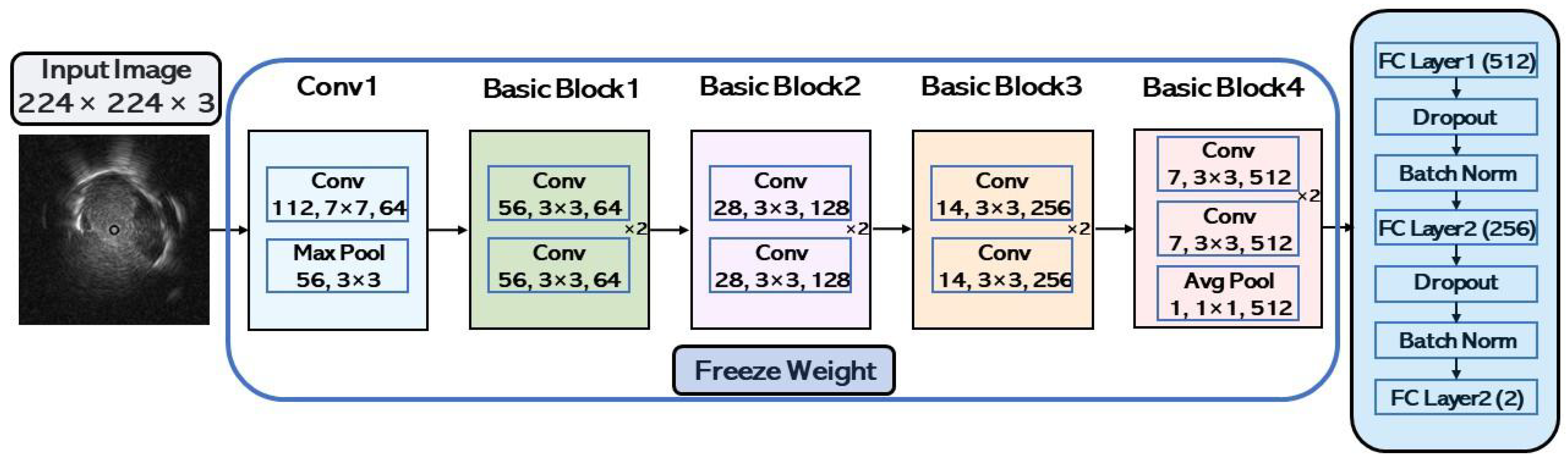
All bagging ensemble experiment result are shown in Table 5, Table 6 and Table 7. Three fusion methods were used in the bagging experiment. Table 5 displays the bagging experimental results with the majority voting fusion method, and Table 4 presents the baseline experimental results. Even with data augmentation to alleviate the imbalanced dataset’s impact, the ResNet-34 backbone did not perform well. One explanation may be that the number of benign cases was insufficient; both baseline and bagging ensemble results evidenced that the PPV was better than the NPV. These findings indicate that trained CNN models can more accurately differentiate malignant cases than benign ones. Notably, the number of malignant cases was much larger than the benign cases in this study; thus, the trained CNN models acquired more knowledge regarding malignant cases than benign ones. Additional benign case data should be collected for future investigations.

Table 6 shows the bagging results with the output average fusion method. The output average fusion method yielded the best results within the ensemble experimental results of three fusion methods and aggregating the same CNN models. A ResNet-18 backbone and two-CNN model combination revealed good results: 0.70 accuracy, 0.63 F1-Score, 0.70 AUC, 0.87 PPV, 0.67 NPV, 0.56 sensitivity, and 0.84 specificity. Table 7 displays the bagging results with the performance weighting fusion method. When aggregating two or three same CNN models, the ResNet-18, ResNet-34, DenseNet-121, and MobileNet-V2 accuracies were remarkably similar. Among all experimental results, a ResNet-18 backbone and the performance weighting fusion method yield the best specificity value, as shown in Table 7.

Based on the comparison results between the best baseline and bagging ensemble results (Table 8), the benign and malignant PPL classification improved. This study conducted five-fold cross-validation to evaluate the proposed CAD system’s performance further. The dataset division results are presented in Table 3. Although the CNN models performed well in some folds, this was not the case for others. This finding reveals that the data distribution of the five-fold dataset was not the same, as using the same CNN model backbone indicated significant differences between results. Another concern involves using pre-trained CNN models for feature extraction. The training results were considerably better than the validation and testing results, potentially due to the CNN models’ depth. In addition, compared with ImageNet images, EBUS is more practical. Deep CNN models are not necessary for feature extraction; therefore, we intend to construct shallow convolutional layers for feature extraction in the future. In addition to using the fully connected layers, we will explore SVM, decision trees, and random forests as classifiers.

Benign or malignant PPLs cannot be determined solely based on EBUS images in clinical practice, as the image features cannot be adequately observed. Thus, a biopsy is often performed to distinguish the PPL type. Despite the developed CAD system’s remarkable performance, there were some limitations. Our study assessed six models and utilized ensemble learning to improve performance, specifically integrating three distinct models. However, numerous excellent deep learning and machine learning algorithms can still be applied to our study. For example, we will explore the fusion of machine learning and deep learning algorithms in our future experiments. We also intend to ensemble a CNN with other state-of-the-art models. Another hurdle was the limited sample size in this study, which impedes our CAD framework’s reliability and performance generalization. External validation is required to address this issue in the future. We will investigate how our system performs when provided data from different hospitals or machine types to validate our proposed model’s reliability and practicality further. This study referenced investigations conducted by other researchers to support our findings and provide a broader context for our research. As such, we also aim to establish a comparison with these references to validate their results using our dataset and further evaluate our model. Lastly, a shallow CNN model should be designed to compare performance with transfer learning.

5.2. Conclusions

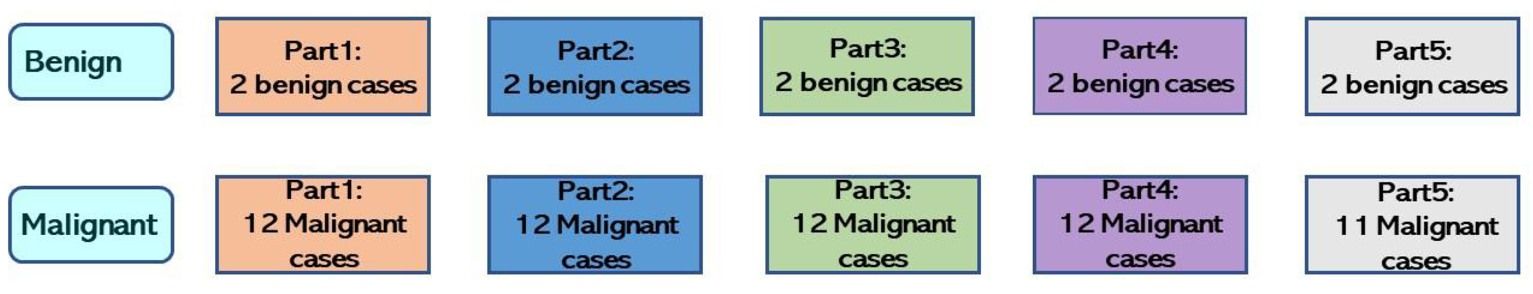
This study developed a computer-aided diagnosis system to differentiate between benign and malignant lung cancer cases from EBUS images. Bagging ensemble learning and down-sampling techniques were applied to our CAD system to resolve an imbalanced dataset and enhance results. As there were far more malignant than benign cases, the malignant cases were down-sampled to consider the entire dataset. Malignant cases were equally divided into three, and each was combined with all the benign cases to create three small datasets. Models were trained with each small dataset and aggregated with the bagging ensemble learning method. Thus, the three trained models contained knowledge for reliable benign and malignant classification. In addition, the three fusion methods were majority voting, output average, and performance weighting. The performance weighting fusion method provided the best bagging ensemble result, achieving a 0.7 accuracy, 0.63 F1-Score, 0.75 AUC, 0.84 PPV, 0.68 NPV, 0.56 sensitivity, and 0.85 specificity.

In conclusion, our proposed computer-aided diagnosis system based on deep learning achieved promising results for diagnosing benign and malignant peripheral pulmonary lesions from endobronchial ultrasonography. However, the dataset used in this study was imbalanced. Excluding data augmentation, we will gather additional PPLs data to verify the CAD system’s efficacy in future studies.

References

1. Pizzato, M.; Li, M.; Vignat, J.; Laversanne, M.; Singh, D.; La Vecchia, C.; Vaccarella, S. The epidemiological landscape of thyroid cancer worldwide: GLOBOCAN estimates for incidence and mortality rates in 2020. Lancet Diabetes Endocrinol. 2022, 10, 264–272. [Google Scholar] [CrossRef] [PubMed]
2. Alberg, A.J.; Brock, M.V.; Ford, J.G.; Samet, J.M.; Spivack, S.D. Epidemiology of Lung Cancer: Diagnosis and Management of Lung Cancer, 3rd ed: American College of Chest Physicians Evidence-Based Clinical Practice Guidelines. Chest 2013, 143, e1S–e29S. [Google Scholar] [CrossRef] [Green Version]
3. Khomkham, B.; Lipikorn, R. Pulmonary Lesion Classification Framework Using the Weighted Ensemble Classification with Random Forest and CNN Models for EBUS Images. Diagnostics 2022, 12, 1552. [Google Scholar] [CrossRef]
4. Chen, C.H.; Lee, Y.W.; Huang, Y.S.; Lan, W.R.; Chang, R.F.; Tu, C.Y.; Chen, C.Y.; Liao, W.C. Computer-aided diagnosis of endobronchial ultrasound images using convolutional neural network. Comput. Methods Programs Biomed. 2019, 177, 175–182. [Google Scholar] [CrossRef]
5. Zhan, P.; Zhu, Q.Q.; Miu, Y.Y.; Liu, Y.F.; Wang, X.X.; Zhou, Z.J.; Jin, J.J.; Li, Q.; Sasada, S.; Izumo, T.; et al. Comparison between endobronchial ultrasound-guided transbronchial biopsy and CT-guided transthoracic lung biopsy for the diagnosis of peripheral lung cancer: A systematic review and meta-analysis. Transl. Lung Cancer Res. 2017, 6, 23. [Google Scholar] [CrossRef] [PubMed] [Green Version]
6. Lou, L.; Huang, X.; Tu, J.; Xu, Z. Endobronchial ultrasound-guided transbronchial needle aspiration in peripheral pulmonary lesions: A systematic review and meta-analysis. Clin. Exp. Metastasis 2022, 40, 45–52. [Google Scholar] [CrossRef]
7. Hearst, M.A.; Dumais, S.T.; Osuna, E.; Platt, J.; Scholkopf, B. Support vector machines. IEEE Intell. Syst. Their Appl. 1998, 13, 18–28. [Google Scholar] [CrossRef] [Green Version]
8. Breiman, L. Random forests. Mach. Learn. 2001, 45, 5–32. [Google Scholar] [CrossRef] [Green Version]
9. Kuruvilla, J.; Gunavathi, K. Lung cancer classification using neural networks for CT images. Comput. Methods Programs Biomed. 2014, 113, 202–209. [Google Scholar] [CrossRef] [PubMed]
10. Alakwaa, W.; Nassef, M.; Badr, A. Lung cancer detection and classification with 3D convolutional neural network (3D-CNN). Int. J. Adv. Comput. Sci. Appl. 2017, 8, 409–417. [Google Scholar] [CrossRef] [Green Version]
11. Chaunzwa, T.L.; Hosny, A.; Xu, Y.; Shafer, A.; Diao, N.; Lanuti, M.; Christiani, D.C.; Mak, R.H.; Aerts, H.J. Deep learning classification of lung cancer histology using CT images. Sci. Rep. 2021, 11, 5471. [Google Scholar] [CrossRef]
12. Nasrullah, N.; Sang, J.; Alam, M.S.; Mateen, M.; Cai, B.; Hu, H. Automated lung nodule detection and classification using deep learning combined with multiple strategies. Sensors 2019, 19, 3722. [Google Scholar] [CrossRef] [Green Version]
13. Chen, J.; Zeng, H.; Zhang, C.; Shi, Z.; Dekker, A.; Wee, L.; Bermejo, I. Lung cancer diagnosis using deep attention-based multiple instance learning and radiomics. Med. Phys. 2022, 49, 3134–3143. [Google Scholar] [CrossRef]
14. He, K.; Zhang, X.; Ren, S.; Sun, J. Deep residual learning for image recognition. In Proceedings of the IEEE Conference on Computer Vision and Pattern Recognition, Las Vegas, NV, USA, 27–30 June 2016; pp. 770–778. [Google Scholar]
15. Huang, G.; Liu, Z.; Van Der Maaten, L.; Weinberger, K.Q. Densely connected convolutional networks. In Proceedings of the IEEE Conference on Computer Vision and Pattern Recognition, Honolulu, HI, USA, 21–26 July 2017; pp. 4700–4708. [Google Scholar]
16. Sandler, M.; Howard, A.; Zhu, M.; Zhmoginov, A.; Chen, L.C. Mobilenetv2: Inverted residuals and linear bottlenecks. In Proceedings of the IEEE Conference on Computer Vision and Pattern Recognition, Salt Lake City, UT, USA, 18–23 June 2018; pp. 4510–4520. [Google Scholar]
17. Ma, N.; Zhang, X.; Zheng, H.T.; Sun, J. Shufflenet v2: Practical guidelines for efficient cnn architecture design. In Proceedings of the European Conference on Computer Vision (ECCV), Munich, Germany, 8–14 September 2018; pp. 116–131. [Google Scholar]
18. Hinton, G.E.; Srivastava, N.; Krizhevsky, A.; Sutskever, I.; Salakhutdinov, R.R. Improving neural networks by preventing co-adaptation of feature detectors. arXiv 2012, arXiv:1207.0580. [Google Scholar]
19. Ioffe, S.; Szegedy, C. Batch normalization: Accelerating deep network training by reducing internal covariate shift. Proc. Mach. Learn. Res. 2015, 37, 448–456. [Google Scholar]
20. Kingma, D.P.; Ba, J. Adam: A method for stochastic optimization. arXiv 2014, arXiv:1412.6980. [Google Scholar]
21. Tibshirani, R. Regression shrinkage and selection via the lasso. J. R. Stat. Soc. Ser. B Methodol. 1996, 58, 267–288. [Google Scholar] [CrossRef]
22. Vidaurre, D.; Bielza, C.; Larranaga, P. A survey of L1 regression. Int. Stat. Rev. 2013, 81, 361–387. [Google Scholar] [CrossRef]
23. Van Laarhoven, T. L2 regularization versus batch and weight normalization. arXiv 2017, arXiv:1706.05350. [Google Scholar]
24. He, H.; Garcia, E.A. Learning from imbalanced data. IEEE Trans. Knowl. Data Eng. 2009, 21, 1263–1284. [Google Scholar]
25. Buda, M.; Maki, A.; Mazurowski, M.A. A systematic study of the class imbalance problem in convolutional neural networks. Neural Netw. 2018, 106, 249–259. [Google Scholar] [CrossRef] [Green Version]
26. Haixiang, G.; Yijing, L.; Shang, J.; Mingyun, G.; Yuanyue, H.; Bing, G. Learning from class-imbalanced data: Review of methods and applications. Expert Syst. Appl. 2017, 73, 220–239. [Google Scholar] [CrossRef]
27. Levi, G.; Hassner, T. Age and gender classification using convolutional neural networks. In Proceedings of the IEEE Conference on Computer Vision and Pattern Recognition Workshops, Boston, MA, USA, 7–12 June 2015; pp. 34–42. [Google Scholar]
28. Elkan, C. The foundations of cost-sensitive learning. In Proceedings of the International Joint Conference on Artificial Intelligence, Seattle, WA, USA, 4–10 August 2001; Volume 17, pp. 973–978. [Google Scholar]
29. Rokach, L. Ensemble-based classifiers. Artif. Intell. Rev. 2010, 33, 1–39. [Google Scholar] [CrossRef]
30. Breiman, L. Bagging predictors. Mach. Learn. 1996, 24, 123–140. [Google Scholar] [CrossRef] [Green Version]
Figure 1. Examples of the benign and malignant peripheral pulmonary lesions in EBUS images. (a,b) are the benign lesions (c,d) are the malignant lesions. The benign and malignant lesions are confirmed by the physicians using a needle biopsy.
Applsci 13 08403 g001
Figure 2. This is a flowchart of the data pre-processing, which describes in detail how the initial EBUS video data is turned into the final dataset used for the experiment. There are 6 steps in the EBUS data pre-processing.
Applsci 13 08403 g002
Figure 3. The example of the original EBUS image converted from the EBUS videos.
Applsci 13 08403 g003
Figure 4. The examples of the EBUS image (a,b) that are screened out from the dataset.
Applsci 13 08403 g004
Figure 5. This is the result of the data augmentation.
Applsci 13 08403 g005
Figure 6. This graph shows how the proposed CAD system works. It consists of three main steps. Firstly, the CAD system performs down-sampling specifically for malignant cases. This down-sampling process helps to reduce the influence of an imbalanced dataset. Secondly, the CAD system utilizes a combination of all the benign cases and an equal number of divided malignant cases to train separate CNN models. Lastly, the CAD system aggregates all the trained CNN models together to generate the final classification result for the input EBUS image. This aggregation step combines the outputs of multiple CNN models, leveraging their collective knowledge and expertise to make a comprehensive and reliable diagnosis.
Applsci 13 08403 g006
Figure 7. This is the architecture of the fine-tuned ResNet-18.
Applsci 13 08403 g007
Figure 8. This figure shows the result of division. For each class, how many cases are in each fold. The total number of benign cases is 10; after division, there are 2 cases in each part. The total number of malignant cases is 59; after division, there are 12 cases in each part, except for the last part.
Applsci 13 08403 g008
Figure 9. The confusion matrix for the baseline and proposed CAD system. (a) shows the confusion matrix for the baseline model using ResNet34, (b) depicts the confusion matrix for the CAD system using the same ResNet34 architecture as the baseline.
Applsci 13 08403 g009