Proactive Mission Planning of Unmanned Aerial Vehicle Fleets Used in Offshore Wind Farm Maintenance

Abstract

This paper presents a declarative model of maintenance logistics for offshore wind farms. Its implementation in decision-making tools supporting wind turbine maintenance enables online prototyping of alternative scenarios and variants of wind turbine servicing, including weather-related operation vessel movement and routing of unmanned aerial vehicle (UAV) fleets carrying out maintenance on these wind turbines during monitoring or component-delivery missions. The possibility of implementing the model was verified via two case studies focusing, separately, on the issues of routing and scheduling of a UAV fleet used for the inspection of wind turbines and the distribution of ordered spare parts. The open structure of the model allows for its easy generalization, expanding the range of supported functions, including vessel fleet routing in an offshore wind farm, staff and competence planning of service teams, and supply chain management, enabling the planning of tool sets distributed to serviced wind turbines. Computer experiments conducted for various weather conditions confirm the competitiveness of the proposed approach.

1. Introduction

The rapid increase in the use of renewable electricity, driven by the development of photovoltaic technologies and wind farms, compels the development of appropriate facilities to ensure their maintenance. Since wind farms are more efficient than traditional sources of electricity and their share in global electricity production is prominent, the development of techniques and maintenance methods dedicated to wind farms will also be prominent [1,2]. Due to their relatively low invasiveness (due to their location outside urban areas), offshore wind turbine farms (OWFs) are particularly important in this sector. OWFs’ locations, especially their accompanying environmental conditions (water conditions, undesirable weather such as fog and rain, etc.), give rise to special requirements and expectations for their maintenance [3].

The rapidly growing number of newly built OWFs and the relatively short service life of wind turbines (WTs) (not exceeding 40 years), as well as the need to shorten their downtime, compel the development of new, efficient maintenance methods, in particular, routine inspection, cleaning, lubrication, and repair of WTs’ main components, including the tower, rotor blades, nacelle, and frames. In general, the problem of OWF maintenance (i.e., the problem of management of maintenance logistics) comes down to the routing and scheduling of the service vessel fleets and service activities performed on WTs by the UAVs and transported service teams [4,5,6]. In other words, it consists of determining the optimal allocation of WTs and routes to vessels, the repair and service teams, and UAV servicing (or supplementing deliveries) for turbines in terms of operating and maintenance (O&M) costs [5,7].

Among the issues dominating OWF maintenance logistics, one can distinguish the issues of vessel route planning and UAV mission planning. Decisions made in these areas influence each other and affect the final costs of WT monitoring/servicing missions. In vessel route planning, a decisive role is played by the choice of vessel route, conditioned by the state of the sea (i.e., maximum allowable significant wave height and peak wave period) and the time taken for a ship to moor at a WT and for the service team to disembark from and return to the vessel. The number of WTs serviced within the planned time window is usually assumed to be its main objective. It is worth adding that both the forecasted weather conditions and daily visibility, conditioned by the year’s season, affect this time window [8,9].

The second issue, UAV mission planning for WT inspection, cleaning, lubrication, and repair, particularly the maintenance of WT main components such as blades, nacelle, and tower, is seeing increasing implementation of UAV technologies because UAVs equipped with a variety of sensors, including ultrasonic, visual, thermographic, and hyperspectral cameras, can detect different types of damage, such as fatigue cracks, surface corrosion, galvanic corrosion, pitting, and stress corrosion cracking [10,11].

Problems in these areas overlap and permeate to several other problems in the logistics of OWF maintenance. Relevant examples include problems such as hierarchical worker assignment (assuming that an employee with a higher competence can replace a lower-skilled employee by performing assigned tasks in a shorter time), supply chain management (using repair kits to service WTs instead of spare parts, separate from the bullwhip effect), and proactive/reactive O&M planning (taking into account changes in weather forecasts and sea states, as well as considering various emergency scenarios). Such complex, multifaceted problems integrating processes of different natures and characters are difficult to model and even more difficult to solve. They are problems of the NP-hard class [8,12,13].

This paper’s subject matter references our previous work addressing the issues of proactive and reactive mission planning of a fleet of UAVs carrying out deliveries in changing weather conditions and ad hoc changing sizes and timing of orders. Thus, the studies presented are an attempt to transfer previously gained experience to an environment in which, in addition to atmospheric disturbances, uncertainties caused by the sea’s changing state (while conditioning the movement of ships used as mobile UAV bases) are considered. Our contribution in this respect consists of the following:

• A declarative reference model of OWF maintenance logistics enabling the integration of operation vessel routing and scheduling problems with UAV delivery and monitoring mission planning problems;
• Procedures for proactive/reactive cruise planning of vessel mooring to selected WTs, including when service teams disembark and return to the vessel, as well as the use of drones for delivery and monitoring purposes;
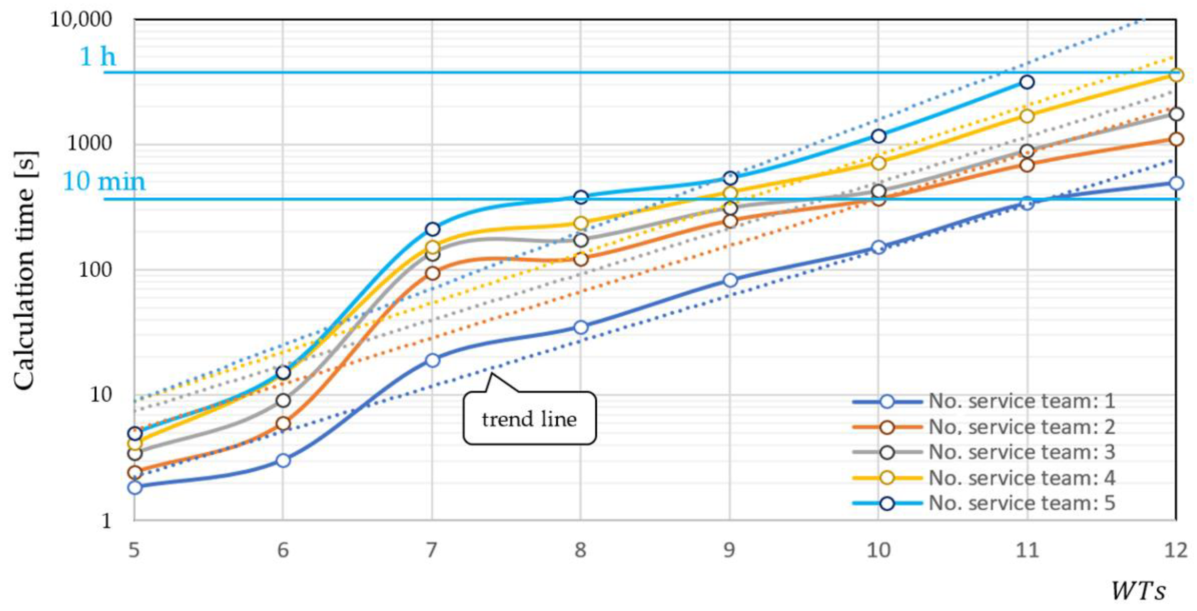
• The results of many computer experiments, illustrating the possibility of using the presented approach to generate alternative scenarios of OWF maintenance logistics, as well as its scalability.

To sum up, the novelty of the proposed approach entails the presentation of two benefits of adopting a reference model. The first is related to the model’s open structure, allowing for its further specification and extension. The second comes down to the possibility of formulating and solving so-called synthesis problems (i.e., as opposed to an analysis—answering the question of what happens when). This allows for answers to the following question to be obtained: what requirements for a fleet of ships, a fleet of UAVs, and technical personnel should be met in a given period of time in order to provide services for an assumed number of WTs?

The structure of this study is as follows: Section 2 discusses the related work and determines the research gaps in the literature. Section 3 presents a reference model of maintenance logistics of OWT, in particular a declarative model and a formal (in terms of constraint satisfaction problems) formulation of the problem. The case studies presented in Section 4 cover UAV fleet planning for wind turbine servicing and spare-part distribution. Section 5 sums up the results of the computer experiments for assessing the scalability of the proposed solutions. Directions of future research are suggested in Section 6.

2. Related Work

The logistics and supply chain management of OWF maintenance have a fundamental impact on their availability and, as a result, profitability. The issues of servicing WTs and OWF maintenance, in general, are currently very often discussed in the literature on the subject [13,14,15,16]. Decision-making, including the management of spare-part inventory, the purchase or lease of consumables, the outsourcing of repair services, the organization and planning of maintenance tasks, and the determination of vessel routes, as well as the selection of OWF maintenance strategies are the most frequently addressed areas of research. The main goal of maintenance strategies is to reduce O&M costs and to improve WT reliability. The decisive share in these costs falls on the handling and maneuvering of service operation vessels; the selection, import, and collection of appropriate components (forming repair kits) intended for the repair of planned WTs; and the completion of tasks by service teams and UAV operators.

Much work has been devoted to the problems of routing and scheduling service vessels. The essence of these problems comes down to optimally assigning WTs and routes to the vessels, as well as minimizing costs related to traveling to the respective WTs [1,12,17]. Relatively few studies deal with uncertainties such as weather-related vessel movement to determine operability. The limitations due to changes in weather conditions (particularly, substantial wave heights and wind speeds) strongly determine the accessibility of WTs to service vessels and personnel transfers from the vessel to the WT.

Traditionally, the visual inspection of WTs by experienced technicians is, in addition to being dangerous, very laborious and time-consuming. It is also very resource-intensive. This work can be successfully performed by UAVs equipped with high-resolution cameras that can detect various types of damage, such as fatigue cracks, surface corrosion, galvanic corrosion, pitting, stress corrosion cracking, and erosion.

In addition to monitoring and carrying out minor maintenance repairs, UAVs are increasingly used to transport spare parts and tools from the vessel to the WT requiring repair [3]. Such a UAV-based solution for the delivery of not very heavy loads allows for a reduction in the limitations related to the availability (e.g., in the case of mooring) of vessels and the dependence on meteorological and environmental conditions. The main limitation of this type of application is an electric drive limiting a UAV’s operating time. Examples of research conducted in the field of UAV energy supply management are presented in [4,18,19].

The considered problem of planning service missions involving the routing/scheduling of a vessel transporting service teams and UAVs delivering spare parts to serviced WTs is a special case of ground–vehicle and unmanned aerial vehicle routing problems (GV-UAV) [20], assuming that the UAVs’ base is an object moving on land. In the literature, there are numerous contributions dealing with this subject [21,22,23,24,25]. However, they do not address the issues of planning missions in a maritime environment, where weather conditions are of great importance to these missions. From this perspective, the proposed declarative model for planning WT service missions fills the gap in the research on the use of UAVs in maritime environments.

The models and methods used in OWF maintenance vary depending on the tasks undertaken each time. The algorithms implemented in these build upon previous experience gained in solving problems arising in a variety of UAV applications, ranging from precision farming [26] to disaster management [27] and infrastructure inspection [28], as well as in various other fields, including the defense, civilian, and commercial sectors. They include stochastic models related to, for example, forecasting service windows, periodic inspections, and organization of supply chains; operational research models (based on mixed-integer programming, dynamic programming, etc.); simulation models (used to determine the trajectory of UAV flight ship routes, etc.); and artificial intelligence models and fuzzy models (using, e.g., population algorithms such as ant colony [29], beetle swarm [30], and system-improved grey wolf optimization [31], as well as fuzzy logic algorithms such as fuzzy reinforcement learning [32], fuzzy particle swarm optimization [33,34], and fuzzy C-means [35]). Formal representations of these models implemented in the relevant methods of imperative programming allow for formulating and solving problems related to the so-called analysis of a problem situation, i.e., related to the search for an answer to the question of whether (what) set values of a set of decision variables guarantee a specific (extreme) value of the assumed objective function. This means that searching for answers related to the so-called synthesis of a problem situation, i.e., related to the search for an answer to the question of whether there are (and if so, what) such values of set decision variables at which the adopted objective function reaches a specific (extreme) value, is not allowed.

Moreover, none of the detailed models presented earlier meet the requirements for use both in the construction of an integrated model of OWF maintenance and in the formulation of synthesis-type problems. Models implementing the declarative programming paradigm have the greatest chance of meeting these expectations. The constraint-programming strategies used in these models enable the formulation of both analysis and synthesis problems due to these models inherently having open structures.

Unfortunately, the declarative approach is very rarely used both for modeling and solving OWF logistics problems. This deficiency is visible, among others, in the need for studies covering reactive OWF maintenance planning, related to the generation of scenarios that would suspend or stop an initiated inspection and/or repair missions. The presented research gap is address by relatively few studies [17,36,37,38]. It is easy to see that filling this gap will contribute to the creation of systems supporting the dispatcher in planning missions related to the maintenance of OWFs.

3. Model Formulation

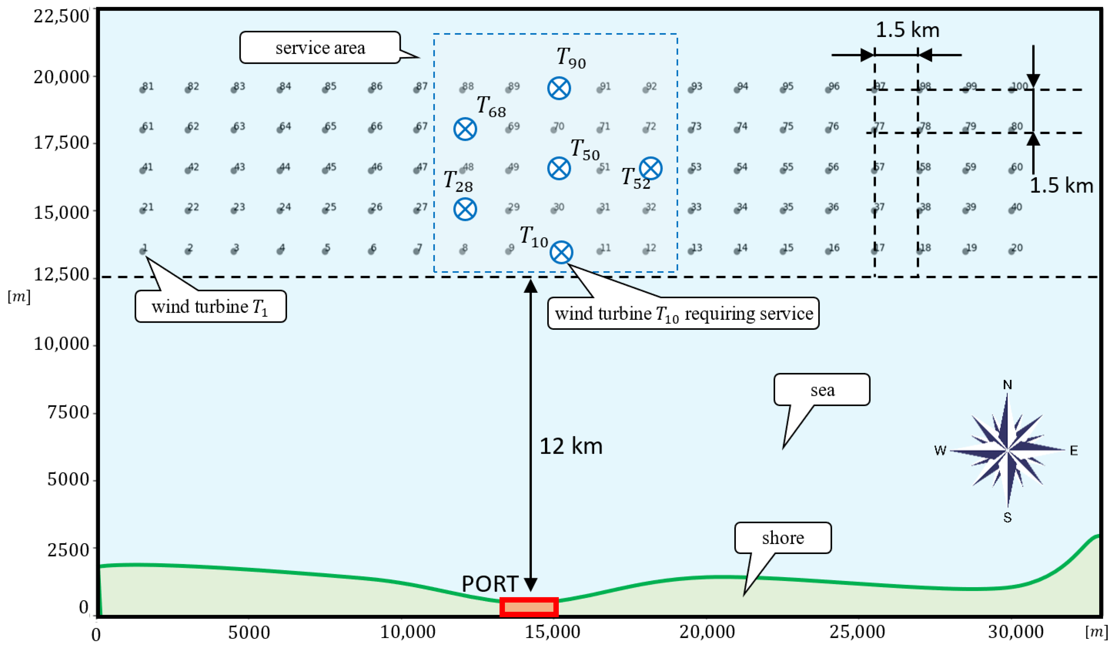
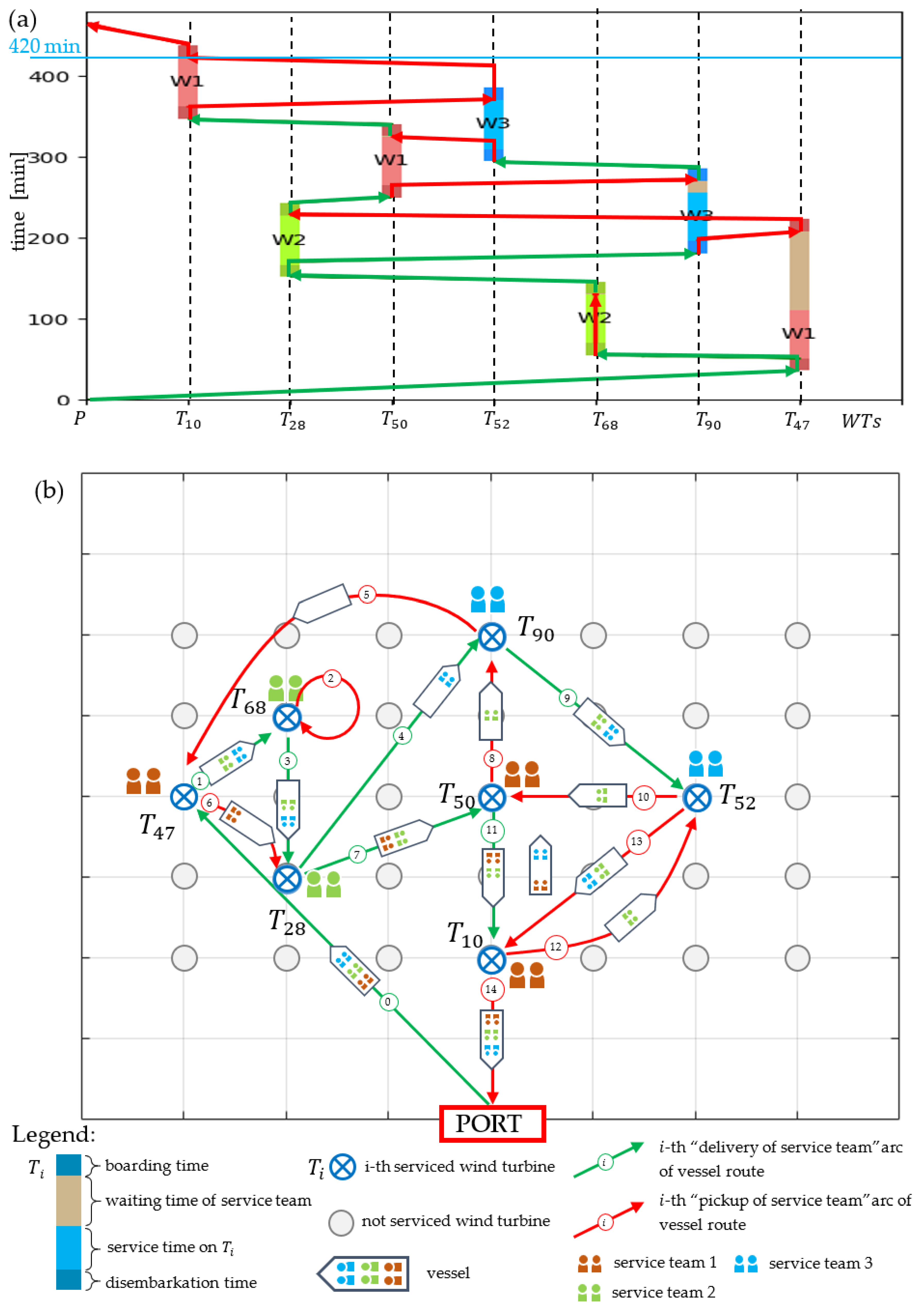
3.1. Illustrative Example

Consider an offshore wind farm with an area of 346.5 ha consisting of 100 WTs with a rotor diameter of 250 m; hereinafter, the turbines are denoted by $T_i$. The turbines are arranged according to the scheme presented in Figure 1. It is assumed that the distance between the WTs is a multiple of the rotor diameter and is equal to 1500 m. Due to the coastal fauna as well as aesthetic conditions, the farm is located 12 km from the shore.

Consider a situation in which 6 WTs, $T=\left\{T_{10},T_{28},T_{50},T_{52},T_{68},T_{90}\right\}$, await technical inspection (repairs) and are located in the service area (marked as blue crossed circles in Figure 1).

It is assumed that the servicing time is equal to 60 min: $t=60 \mathrm{m}\mathrm{i}\mathrm{n}$. There are 3 service teams available, $W=\left\{W_1, W_2, W_3\right\}$, each consisting of a pair of employees. Each service team has different competences. The level of competence of the team has an impact on the service activities performed by them. The difference in competence is reflected in the cost of employing a given team for the service. The impact on the time-of-service task and the cost of a given group is presented in

Table 1. Characteristics of the service teams.

	Effect on Nominal Operation Time [min]	Cost of an Employee Performing a Service Order [u.m./h]	The Cost of an Employee Waiting for a Service Order [u.m./h]
$W_1$	−15	60	50
$W_2$	0	40	30
$W_3$	15	20	10

.

It is required that all turbines of the $T$ set undergo service within 1 working day, i.e., that the duration of the entire mission does not exceed $H=8 \mathrm{h}$ (each WT can be serviced by any of the service teams, i.e., a subset of the set $W$).

The transport of service teams to turbines is carried out via a vessel. The vessel sails at an average speed of 8 m/s. The cost of the vessel’s operating hour is $csa=120$ [u.m./h] (u.m. = units of money), while the cost of parking the vessel (e.g., when employees descend from the ship to the WT) $csp=60$ [u.m./h].

Moreover, it is assumed that the time of descent of employees from the ship to the WT, as well as the time of return from the WT to the ship, is $TI=15 \mathrm{m}\mathrm{i}\mathrm{n}$.

During a service operation, it may be necessary to deliver additional components (e.g., spare parts and tools) from the vessel to the WT. The vessel is equipped with a UAV, $u_1$ (with the technical parameters described in

Table 2. Technical parameters of the used UAV.

UAV	Max Speed [m/s]	Weight Capacity [kg]	Load/Unload Time [min]	Cost [u.m./h]
$u_1$	16	120	10	50

), which is responsible for delivering the ordered goods.

In this context, maintenance mission planning includes, on the one hand, ship mission planning and the assignment of service teams to WTs and, on the other hand, planning of the delivery of components (by the UAV) during the service of these WTs. Therefore, the problem of planning service missions can be reduced to the following two stages:

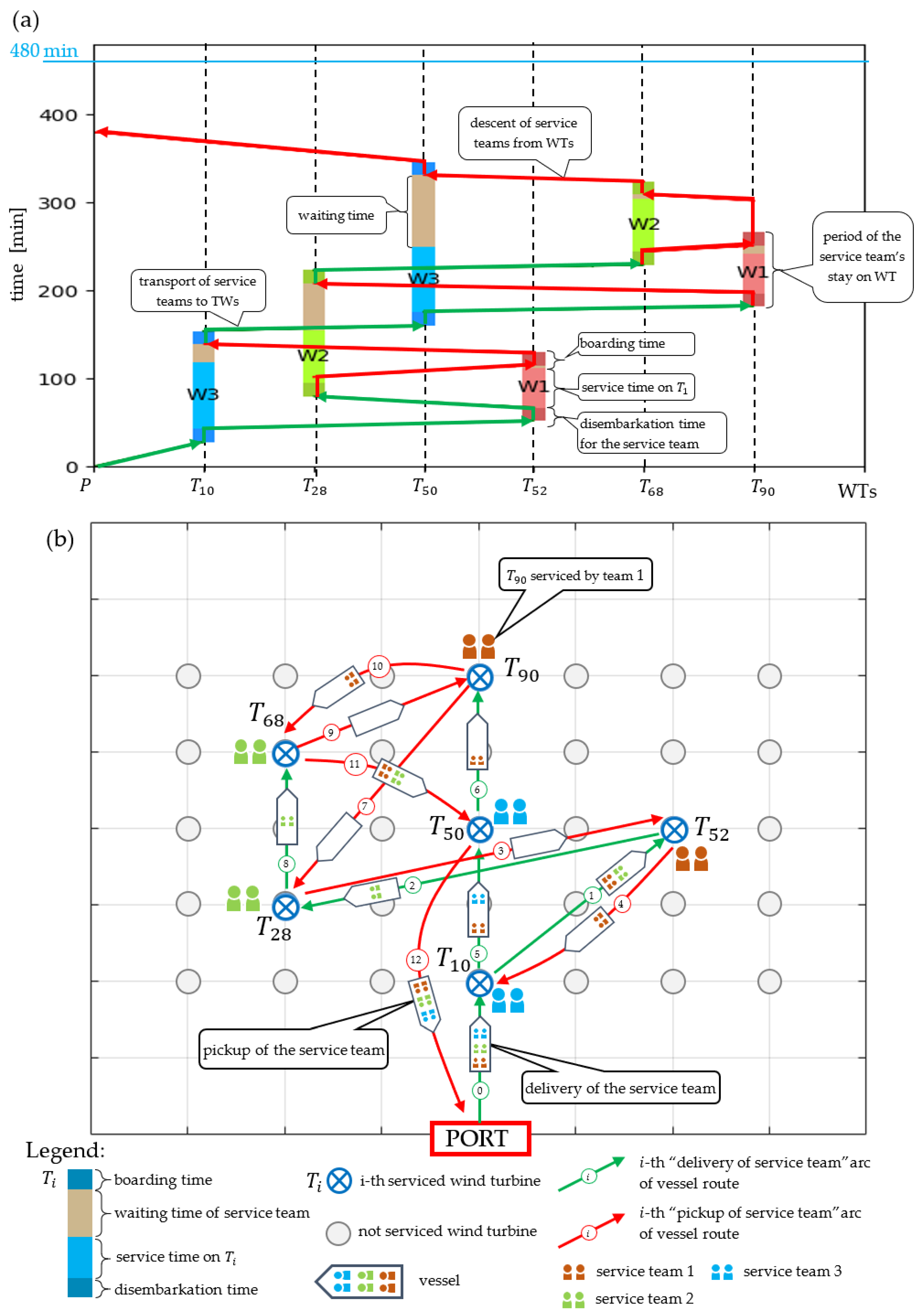
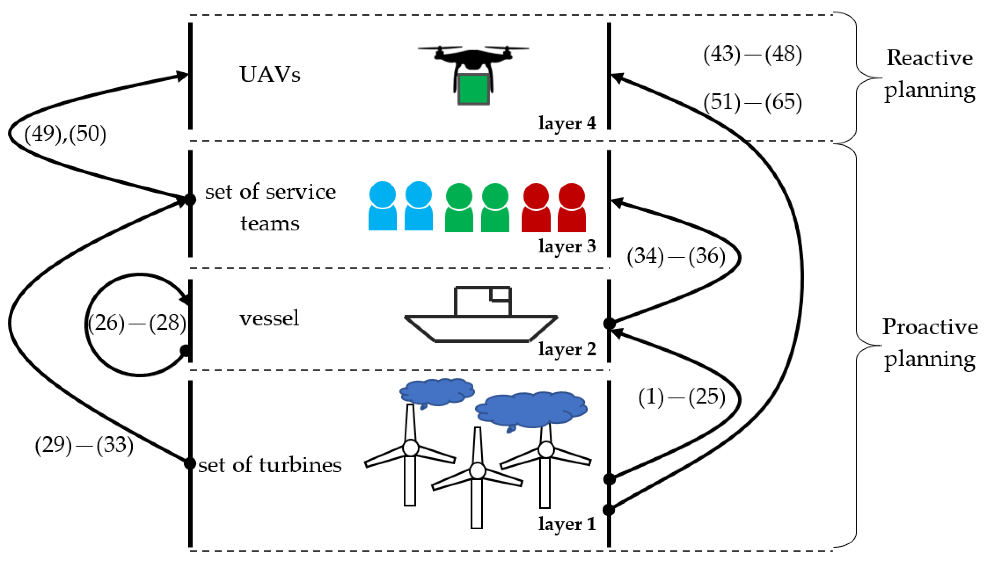
• Proactive planning: The pre-mission stage in which the vessel’s route and the assignment of service teams to WTs are planned. Only teams responsible for servicing turbines are considered.
  The vessel’s mission is determined, guaranteeing minimal cost of servicing a given set of WTs by a given set of service teams.
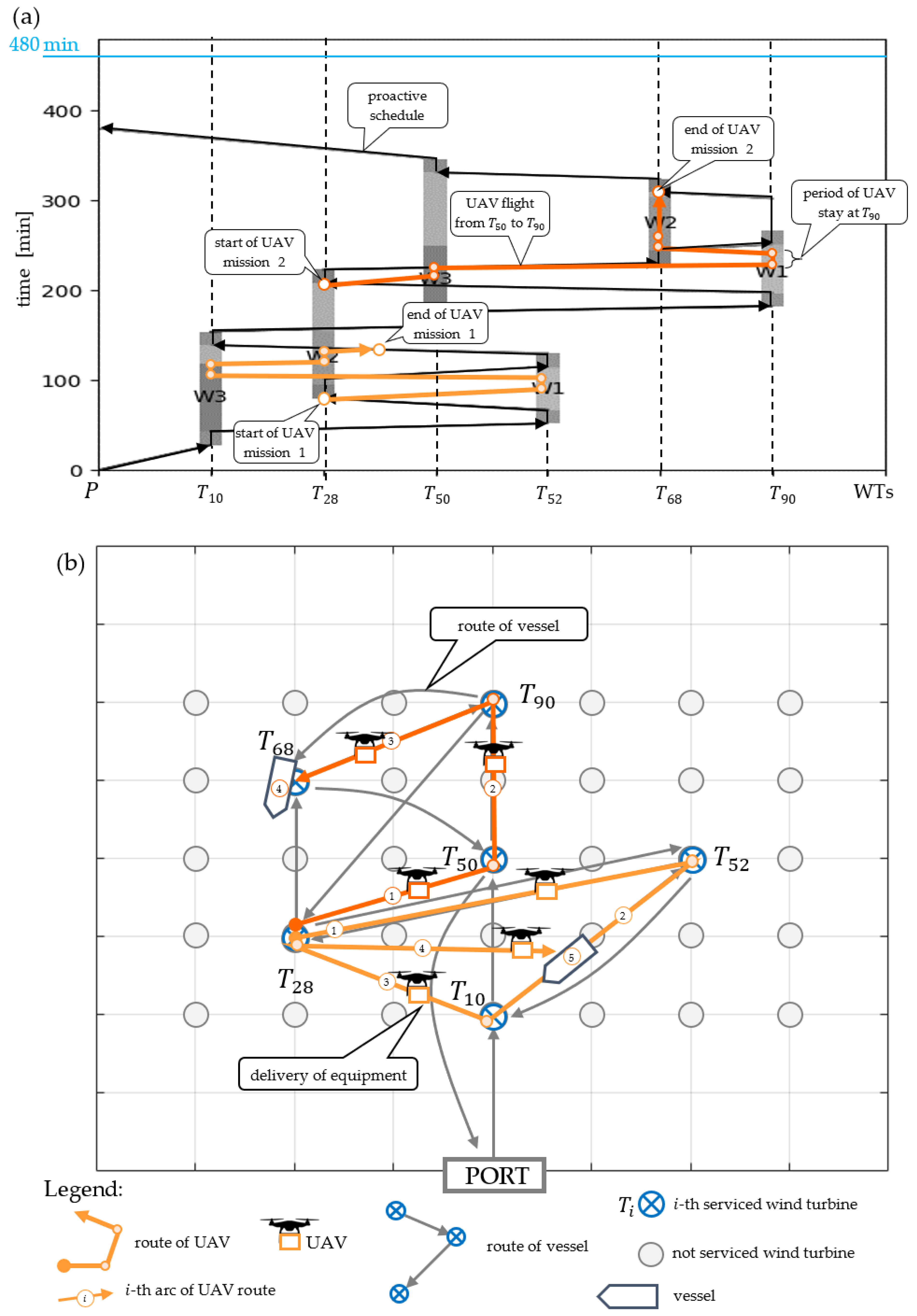
• Reactive planning: This stage is carried out during the implementation of the mission. During the mission, requests are received from service teams (servicing WTs) regarding spare parts required for delivery to WT. A fleet of UAVs and service teams are available on the vessel. The position of the vessel, its route, and the weather conditions are known.

A UAV mission is planned to ensure the timely delivery of expected goods to WT service teams.

Planning the individual stages of the service mission assumes the following:

• The set $T$ of WTs that require service (specified by data such as WT position, estimated service time, and WT demand for parts transported by UAVs) is known.
• The fleet of vessels $V$ transporting service teams (in the considered case, the fleet contains only one vessel), specified by technical data such as vessel travel times between WTs and the base (port) and the costs of vessel usage (distinguishing two kinds of cost: one when the ship is traveling and the second when the ship is moored, e.g., during boarding/disembarking operations of service teams), is known.
• The service teams, as subsets of the set $W$ (specified by data such as the competence of the service personnel, the costs associated with employment, and the approximate times needed to perform the same activity), are known.
• The available fleet $U$ of UAVs transporting parts to the WT (in the considered case, the fleet contains only one UAV), specified by technical data about the UAVs and their cost of usage, are known.
• All assumed WTs (from a set $T$) must be serviced.
• One team of technicians can service only one WT at a time.
• Parts for WTs should be delivered when the work is carried out by the service team.
• Milk-run UAV routes are allowed (UAVs can deliver and receive parts for several WTs (i.e., pick and place mode) as long as the cumulative weight of the components does not exceed the weight capacity).
• The requirements for WT spare parts are known in advance.

An illustration of a proactive mission plan (determined before it begins) is shown in Figure 2a,b. The first subfigure presents a schedule of service activities that guarantees their completion before the assumed planning horizon $H=8 \mathrm{h}$. Along the X-axis, there are serviced turbines, while the Y-axis represents time. Figure 2b depicts the route of a vessel that distributes and receives service teams $W_1, W_2, {\mathrm{a}\mathrm{n}\mathrm{d} W}_3$. The vessel first sails to $T_{10}$ and leaves service team 3 there; then sails to $T_{52}$, where it leaves team 1; then sails to ${\mathrm{T}}_{28}$, where it leaves team 3; and so on until the mission is completed. The mission duration is equal to $MD=386$ min and the costs is $C=1466$m.u.

For such a designated mission, two deadlines are set for the delivery of equipment necessary to service the turbines. At $t=65$ $\mathrm{m}\mathrm{i}\mathrm{n}$, the WT equipment supply window starts, $T_{10}$, $T_{28}$, and $T_{52}$; at $t=200 \mathrm{m}\mathrm{i}\mathrm{n}$, the WT supply window begins, $T_{50}$, $T_{68}$, and $T_{90}.$ An example of a plan for the supply of WT equipment using the available UAV ($u_1$) is presented in Figure 3, illustrating the reactive planning approach. The UAV carries out two missions. In the first one (starting at the 65th minute), the UAV flies to $T_{52}$, then $T_{10}$, and then $T_{28}$. In the second mission (starting at the 200th minute), the UAV flies to $T_{50}$, then $T_{90}$, and then $T_{68}$.

It is easy to see how the problem combines issues in the field of routing a fleet of vessels $V$ and a fleet of UAVs $U$, as well as scheduling service operations executed by delegated teams (in general, the considered problem belongs to the NP-hard class). The distinction between the stages of proactive and reactive mission planning for offshore wind farm maintenance in a natural manner gives it a layered, hierarchical structure, affecting the way it can be solved.

3.2. Declarative Model Description

In the structure of the modeled system, four layers can be distinguished: WTs, vessels, service teams, and UAVs (see Figure 4). These layers interact with each other. For example, the location of the WTs (layer 1) determines the vessel’s acceptable sailing routes (layer 2), which in turn determine the possible service team assignments and the schedule for WT servicing (layer 3). The adopted service schedule affects the plan for equipment delivery by UAVs (layer 4), which is also dependent on the weather conditions prevailing at sea (layer 1). These relationships are distinguished by the declarative model presented below.

The analytical representation of this model is directly provided by the declarative modeling paradigm.

Constraints:

• Constraints determining the permissible routes of the vessel:

  $${\sum }_{j=1}^{NI}{dx}_{1,j}=1$$

  (1)

  $${\sum }_{i=1}^{NI}{dx}_{i,1}=0$$

  (2)

  $${dx}_{i,i}=0, \mathrm{for} i=1\dots NI$$

  (3)

  $${\sum }_{i=1}^{NI}{dx}_{i,j}=1, \mathrm{for} j=2\dots NI$$

  (4)

  $${\sum }_{j=1}^{NI}{px}_{1,j}=0$$

  (5)

  $${\sum }_{i=1}^{NI}{px}_{i,1}=1$$

  (6)

  $$\left({\sum }_{i=1}^{NI}{dx}_{i,j}=1\right)\Rightarrow \left({\sum }_{i=1}^{NI}{px}_{i,j}=1\right), \mathrm{for} j=1\dots NI$$

  (7)

  $${\sum }_{j=1}^{NI}\left({dx}_{i,j}+{px}_{i,j}\right)={\sum }_{j=1}^{NI}\left({dx}_{j,i}+{px}_{j,i}\right), \mathrm{for} i=1\dots NI$$

  (8)
• Constraints that, if fulfilled, guarantee the timely delivery and pick-up of service teams:

  $$\left({dx}_{1,j}=1\right)\Rightarrow \left(\overline{{dy}_j}={vt}_{1,j}\right), \mathrm{for} j=2\dots NI$$

  (9)

  $$\left({dx}_{1,j}=1\right)\Rightarrow \left(\underset{\_}{{dy}_j}=\overline{{dy}_j}-{vt}_{1,j}\right), \mathrm{for} j=2\dots NI$$

  (10)

  $$\left({dx}_{i,j}=1\right)\Rightarrow \left(\overline{{dy}_j}\ge \overline{{dy}_i}+{vw}_i+{vt}_{i,j}\right), \mathrm{for} j=2\dots NI, i\ne j$$

  (11)

  $$\left({dx}_{i,j}=1\right)\Rightarrow \left(\underset{\_}{{dy}_j}=\overline{{dy}_j}-{vt}_{1,j}-{vw}_i\right), \mathrm{for} i,j=2\dots NI, i\ne j$$

  (12)

  $$\overline{{dy}_i}\le H, \mathrm{for} i=1\dots NI$$

  (13)

  $$\left({px}_{i,1}=1\right)\Rightarrow \left(\overline{{py}_1}=\overline{{py}_i}+{vt}_{i,1}\right), \mathrm{for} i=2\dots NI$$

  (14)

  $$\left({px}_{i,1}=1\right)\Rightarrow \left(\underset{\_}{{py}_1}=\overline{{dy}_1}-{vt}_{i,1}\right), \mathrm{for} i=2\dots NI$$

  (15)

  $$\left({px}_{i,j}=1\right)\Rightarrow \left(\overline{{py}_j}\ge \overline{{dy}_i}+{vw}_i+{vt}_{i,j}\right), \mathrm{for} i,j=2\dots NI, i\ne j$$

  (16)

  $$\left({px}_{i,j}=1\right)\Rightarrow \left(\underset{\_}{{py}_j}=\overline{{py}_j}-{vt}_{i,j}-{vw}_i\right), \mathrm{for} i,j=2\dots NI, i\ne j$$

  (17)

  $$\left({px}_{i,i}=1\right)\Rightarrow \left(\underset{\_}{{py}_i}=\overline{{dy}_i}\right), \mathrm{for} i=1\dots NI$$

  (18)

  $$\left({dx}_{i,j}=1\right)\wedge \left({px}_{i,i}=1\right)\Rightarrow \left(\underset{\_}{{dy}_j}\ge \overline{{py}_i}\right), \mathrm{for} i,j=2\dots NI, i\ne j$$

  (19)

  $$\left({px}_{i,j}=1\right)\wedge \left({px}_{i,i}=1\right)\Rightarrow \left(\underset{\_}{{py}_j}\ge \overline{{py}_i}\right), \mathrm{for} i,j=2\dots NI, i\ne j$$

  (20)

  $$\left({dx}_{k,i}=1\right)\wedge \left({dx}_{k,j}=1\right)\Rightarrow \left(\underset{\_}{{dy}_i}\ge \overline{{py}_k}\right)\vee \left(\underset{\_}{{dy}_j}\ge \overline{{py}_k}\right), \mathrm{for} k,i,j=2\dots NI$$

  (21)

  $$\left({dx}_{k,i}=1\right)\wedge \left({px}_{k,j}=1\right)\Rightarrow \left(\underset{\_}{{dy}_i}\ge \overline{{py}_k}\right)\vee \left(\underset{\_}{{py}_j}\ge \overline{{py}_k}\right), \mathrm{for} k,i,j=2\dots NI$$

  (22)

  $$\left({px}_{k,i}=1\right)\wedge \left({px}_{k,j}=1\right)\Rightarrow \left(\underset{\_}{{py}_i}\ge \overline{{py}_k}\right)\vee \left(\underset{\_}{{py}_j}\ge \overline{{py}_k}\right), \mathrm{for} k,i,j=2\dots NI$$

  (23)

  $$\overline{{py}_i}\le H, \mathrm{for} i=1\dots NI$$

  (24)

  $$\overline{{py}_i}\ge \overline{{dy}_i}+{st}_i, \mathrm{for} i=2\dots NI$$

  (25)

  $$\left(\overline{{dy}_i}\le \underset{\_}{{dy}_j}\right)\vee \left(\overline{{dy}_j}\le \underset{\_}{{dy}_i}\right), \mathrm{for} i,j=2\dots NI, i\ne j$$

  (26)

  $$\left(\overline{{py}_i}\le \underset{\_}{{py}_j}\right)\vee \left(\overline{{py}_j}\le \underset{\_}{{py}_i}\right), \mathrm{for} i,j=2\dots NI, i\ne j$$

  (27)

  $$\left(\overline{{py}_i}\le \underset{\_}{{dy}_j}\right)\vee \left(\overline{{dy}_j}\le \underset{\_}{{py}_i}\right), \mathrm{for} i,j=2\dots NI, i\ne j$$

  (28)
• Constraints determining the allocation of service teams to WTs and the schedule of tasks carried out by them in a given time horizon:

  $$\left({aw}_{\omega ,i}=1\right)\Rightarrow \left({st}_i={nt}_i+s{f}_{\omega }\right), \mathrm{for} i=1\dots NI, \omega =1\dots NW$$

  (29)

  $$s{f}_1=0$$

  (30)

  $${\sum }_{\omega =1}^{NW}{aw}_{\omega ,i}=1, \mathrm{for} i=2\dots NI$$

  (31)

  $${\sum }_{\omega =1}^{NW}{aw}_{\omega ,1}=0$$

  (32)

  $${\sum }_{i=2}^{NI}{aw}_{\omega ,i}\ge 1, \mathrm{for} \omega =1\dots NI$$

  (33)

  $$\left(\overline{{sy}_i}\le \underset{\_}{{sy}_j}\right)\vee \left(\overline{{sy}_j}\le \underset{\_}{{sy}_i}\right), \mathrm{for} i,j=2\dots NI, i\ne j$$

  (34)

  $$\underset{\_}{{sy}_i}=\overline{{dy}_i}, \mathrm{for} i=2\dots NI$$

  (35)

  $$\overline{{sy}_i}=\overline{{py}_i}+{vw}_i, \mathrm{for} i=2\dots NI$$

  (36)
• Cost constraints:

  $$\left(d{x}_{i,j}=1\right)\wedge \left(p{x}_{k,j}=1\right)\Rightarrow {sTC}_j=\left(v{t}_{i,j}+v{t}_{k,j}\right)\times \left(\frac{csa}{60}\right), \mathrm{for} i,j,k=1...NI$$

  (37)

  $$\left(d{x}_{i,j}=1\right)\wedge \left(p{x}_{k,j}=1\right)\Rightarrow {sWC}_j=\left(2TI\right)\times \left(\frac{csp}{60}\right), \mathrm{for} i,j,k=1...NI$$

  (38)

  $$\left(a{w}_{\omega ,i}=1\right)\Rightarrow wP{C}_{\omega ,i}=\left(2TI+s{t}_i\right)\times \left(\frac{c{p}_{\omega }}{60}\right), \mathrm{for} i=1..NI,\omega =1\dots NW$$

  (39)

  $$\left(a{w}_{\omega ,i}=1\right)\Rightarrow wW{C}_{\omega ,i}=\left(\overline{{sy}_i}-(\underset{\_}{{sy}_i}+2TI+s{t}_i)\right)\times \left(\frac{c{w}_{\omega }}{60}\right), \mathrm{for} i=1..NI,\omega =1\dots NW$$

  (40)

  $$\left(u{x}_{i,j}=1\right)\Rightarrow uT{C}_j=u{t}_{i,j}\times \left(\frac{cu}{60}\right), \mathrm{for} i,j=1\dots NU$$

  (41)

  $$C={\sum }_{i=1}^{NI}(sT{C}_i+sW{C}_i)+{\sum }_{i=1}^{NU}\left(uT{C}_i\right)+{\sum }_{\omega =1}^{NW}{\sum }_{i=1}^{NI}(wP{C}_{\left(\omega ,i\right)}+w{W}_{\omega ,i})$$

  (42)
• Constraints determining the route and schedule of deliveries carried out by the UAVs:

  $${ux}_{i,i}=0, \mathrm{for} i=1\dots NU$$

  (43)

  $${\sum }_{j=1}^{NU}{ux}_{i,j}=1, \mathrm{for} i=1\dots NU$$

  (44)

  $$\left({ux}_{1,j}=1\right)\Rightarrow \left(\overline{{uy}_j}=\mathrm{s}+{ut}_{1,j}\right), \mathrm{for} i=1\dots NU$$

  (45)

  $$\left({ux}_{i,j}=1\right)\Rightarrow \left(\overline{{uy}_j}=\underset{\_}{{uy}_i}+{ut}_{\mathrm{i},j}\right)\wedge \left(\underset{\_}{{uy}_j}=\overline{{uy}_j}+u{w}_j\right), \mathrm{for} i,j=1\dots NU$$

  (46)

  $$\overline{{uy}_i}\le H\times {\sum }_{j=1}^{NU}{ux}_{i,j}, \mathrm{for} i=1\dots NU$$

  (47)

  $$\underset{\_}{{uy}_i}\le H\times {\sum }_{j=1}^{NU}{ux}_{i,j}, \mathrm{for} i=1\dots NU$$

  (48)

  $$\overline{{uy}_i}\ge \overline{{sy}_i}, \mathrm{for} i=1\dots NU$$

  (49)

  $$\underset{\_}{{uy}_i}\le \overline{{sy}_i}+s{t}_i, \mathrm{for} i=1\dots NU$$

  (50)

  $${\sum }_{j=1}^{NU}{ux}_{i,j}={\sum }_{j=1}^{NU}{ux}_{j,i}, \mathrm{for} i,j=1\dots N.$$

  (51)
• Constraints on the amount of equipment to be supplied:

  $$c_i\le Q\times {\sum }_{j=1}^{NU}{ux}_{j,i}, \mathrm{for} i=1\dots NU$$

  (52)

  $${\sum }_{i=1}^{NU}{c}_i\le Q$$

  (53)

  $$\left({ux}_{i,j}=1\right)\Rightarrow \left(c_i=z_i\right);\mathrm{for} i=1\dots NU$$

  (54)

  $$\left({ux}_{1,j}=1\right)\Rightarrow \left(f{c}_j={\sum }_{i=1}^{NU}{c}_i\right), \mathrm{for} i,j=1\dots NU$$

  (55)

  $$\left({ux}_{i,j}=1\right)\Rightarrow \left(f{c}_j=f{c}_i-z_i\right), \mathrm{for} i,j=1\dots NU$$

  (56)

  $$\left({ux}_{1,j}=1\right)\Rightarrow \left(f_{1,j}={\sum }_{i=1}^{NU}{c}_i\right), \mathrm{for} i,j=1\dots NU$$

  (57)

  $$\left({ux}_{i,j}=1\right)\Rightarrow \left(f_{i,j}=f{c}_j\right), \mathrm{for} i,j=1\dots NU$$

  (58)
• Constraints that, if fulfilled, guarantee the implementation of the desired deliveries in the forecasted weather conditions:

  $${\rm Y}\left(\theta \right)\ge \mathcal{F}\left(\theta \right); \forall \theta \in [0^{\circ },{360}^{\circ })$$

  (59)

  $${\rm Y}\left(\theta \right)=\max \mathsf{\Gamma }\left(\theta \right)$$

  (60)

  $$\mathsf{\Gamma }\left(\theta \right)=\left\{vw|{vw\in R}_{+}^0\wedge bat\left(\theta ,vw\right)\le CAP\right\}$$

  (61)

  $$bat\left(\theta ,vw\right)={\sum }_{i=1}^{NU}{\sum }_{j=1}^{NU}{ux}_{i,j}\times {ut}_{i,j}\times P_{i,j}\left(\theta ,vw\right)$$

  (62)

  $$P_{i,j}(\theta ,vw)=\frac{1}{2}{C}_D\times A\times D\times {\left({va}_{i,j}(\theta ,vw)\right)}^3+\frac{{\left(\left(ep+{\mathrm{f}}_{i,j}\right)\times \mathrm{g}\right)}^2}{D\times b^2\times {va}_{i,j}{(\theta ,vw)}^{’}}$$

  (63)

  where ${va}_{i,j}(\theta ,vw)$ and $u{t}_{i,j}$ depend on the assumed goods delivery strategy.

If the ground speed ${vg}_{i,j}^{ }$ is constant, then an air speed ${va}_{i,j}^{ }$ is calculated from

$${va}_{i,j}(\theta ,vw)=\sqrt{{\left({vg}_{i,j}^{}\times cos{\vartheta }_{i,j}-vw\times cos{\theta }_{}\right)}^2+{\left({vg}_{i,j}^{}\times sin{\vartheta }_{i,j}-vw\times sin{\theta }_{}\right)}^2}$$

(64)

$$u{t}_{i,j}=d_{i,j}/{vg}_{i,j}^{}$$

(65)

The function $\mathcal{F}\left(\theta \right)$ (used in (59)) represents the forecasted weather conditions during the UAV flight mission [38,39]. A value of this function determines the maximal value of forecasted wind speed $vw$ in direction $\theta$. Moreover, the function ${\rm Y}\left(\theta \right)$ determines the robustness of a UAV flight mission plan for the forecasted weather conditions [40]. This means that its value determines the border value of wind speed $vw$ in direction $\theta$ for which the UAV flight mission plan is feasible (i.e., the duration of the mission will not fully discharge the UAV’s battery).

3.3. Problem Statement

The introduced model allows for defining two kinds of problems:

• The analysis problem comes down to searching for answers to the following questions: Do the available resources (vessels, service teams, and UAV fleets) allow for the servicing of a given set of $T$ WTs in the assumed time horizon $H$? And, if so, what is the service plan that guarantees minimal cost $C$?
• The synthesis problem comes down to the search for an answer to the following question: What is/are the structure/parameters of the used resources (vessels, service teams, and UAV fleets) that guarantee the service of a given set of $T$ WTs in the assumed time horizon $H$ and the given cost $C$?

The ability to answer the above questions comes down to a solution dedicated to the constraint satisfaction problem (CSP). Depending on the planning stage, this problem is described in (66) and (67):

• For proactive planning:

  $${C{P}_{AP}}_{}=\left({\mathcal{V}}_{AP},{\mathcal{D}}_{AP},{\mathcal{C}}_{AP}\right)$$

  (66)

  where

• ${\mathcal{V}}_{AP}=\{{\Pi }_{AP},Y_{AP},A_{AP},{WY}_{Ap}\}$—a set of decision variables that determine the plan of mission $S_{ }$:

  ○

  ${\Pi }_{AP}—$a set containing the variables of the vessel route: ${\Pi }_{AP}=\left\{{dx}_{i,j},{px}_{i,j}|i,j=1\dots NI\right\}$;

  ○

  $Y_{Ap}$—the schedule of a vessel: $Y_{AP}=\left\{\overline{{dy}_i},\underset{\_}{{dy}_i},\overline{{py}_i},\underset{\_}{{py}_i}|i=1\dots NI\right\}$;

  ○

  $A_{AP}$—an assignment for the service teams: $A_{AP}=\left\{{aw}_{\omega ,i}|\omega =1\dots NW,i=1\dots NI\right\}$;

  ○

  ${WY}_{Ap}$—a schedule for the service teams: ${WY}_{Ap}=\left\{\overline{{sy}_i},\underset{\_}{{sy}_i}|i=1\dots NI\right\}$;

• ${\mathcal{D}}_{AP}$—a finite set of decision variable domain descriptions: $\overline{{dy}_i},\underset{\_}{{dy}_i},\overline{{py}_i},\underset{\_}{{py}_i},\overline{{sy}_i},\underset{\_}{{sy}_i}\in \mathbb{N}$, ${{dx}_{i,j},{px}_{i,j},aw}_{\omega ,i}\in \left\{\mathrm{0,1}\right\}$;
• ${\mathcal{C}}_{AP}—$a set of constraints specifying the relationships between the vessels, service teams and routes, and turbine networks (1)–(42).

• For reactive planning:

  $${C{P}_{AR}}_{}=\left({\mathcal{V}}_{AR},{\mathcal{D}}_{AR},{\mathcal{C}}_{AR}\left({\mathcal{V}}_{AP}\right)\right)$$

  (67)

  where

• ${\mathcal{V}}_{AR}=\{{\Pi }_{AR},Y_{AR}\}$—a set of decision variables that determine the plan of mission $S_{ }$:

  ○

  ${\Pi }_{AR}—$a set containing the variables of the UAV route: ${\Pi }_{AR}=\left\{{ux}_{i,j}|i,j=1\dots NU\right\}$;

  ○

  $Y_{AR}$—the schedule of a UAV: $Y_{AR}=\left\{s,\overline{{uy}_i},\underset{\_}{{uy}_i}|i=1\dots NU\right\}$;

  ○

  $C_{AR}$—the weight of the delivered equipment: $C_{AR}=\left\{c_i|i=1\dots NU\right\}$;

• ${\mathcal{D}}_{AR}$—a finite set of decision variable domain descriptions: $s,\overline{{uy}_i},\underset{\_}{{uy}_i,c_i}\in \mathbb{N}$, ${ux}_{i,j}\in \left\{\mathrm{0,1}\right\}$;
• ${\mathcal{C}}_{AR}\left({\mathcal{V}}_{AP}\right)$—a set of constraints specifying the relationships between the UAVs, transported equipment, and proactive plans ${\mathcal{V}}_{AP}$ (43)–(65).

To solve the ${C{P}_{AP}}_{}$ and $C{P}_{AR}$ defined by Formulas (66) and (67), the values of the decision variables for which all the constraints are satisfied need to be found. For relevant examples of how to implement these problems in IBM ILOG, see the following case studies.

4. Case Study

4.1. Wind Turbine Service

Consider the set of turbines $T=\left\{T_{10},T_{28},T_{50},T_{52},T_{68},T_{90}\right\}$ from the example discussed in Section 3.1, which has been extended by an additional WT $T_{47}$. Due to difficult weather conditions, the time for the maintenance and repair mission was reduced to 7 h. There are three service teams, whose parameters are listed in

Table 3. Characteristics of the service teams in the considered example.

	Effect on Nominal Operation Time [min]	Cost of an Employee Performing a Service Order [u.m./h]	The Cost of an Employee Waiting for a Service Order [u.m./h]
$W_1$	0	40	30
$W_2$	0	40	30
$W_3$	0	40	30

(all teams have the same competencies). For these data, the answer to the following question is sought: Do the available vessels and teams $W_1$, $W_2$, and $W_3$ allow for the servicing of a given set of $T=\left\{T_{10},T_{28},T_{50},T_{52},T_{68},T_{90},T_{47}\right\}$ in the assumed time horizon $H=420$ (7 h)? And, if so, what is the service plan that guarantees minimal cost $C$?

The purpose of the relevant $C{P}_{AP}$ analysis problem (66) implemented in the IBM ILOG environment is to determine a proactive mission plan. The permissible solution obtained during the 300 s calculations guarantees the service of the set of turbines within 466 min (see Figure 5). Despite the fact that the time obtained is the shortest among those obtained for the same data, it does not meet the accepted expectations, i.e., it is not an acceptable solution (service should be finished in the assumed time horizon $H=420$ min).

Because of the lack of an acceptable solution, an attempt was made to determine the composition of the ship’s crew (set $W$) guaranteeing the service of $T$ WTs in the assumed time horizon $H$. In other words, the answer to the following question is sought: Does there exist a set of teams $W$ guaranteeing the service of a given set of $T$ WTs in the assumed time horizon $H$?

It was assumed that the set $W$ may consist of one to five service teams with the parameters specified in Table 3. The considered problem was implemented in the IBM ILOG environment. The obtained solutions are presented in

Table 4. Solving the synthesis problem for $T=\left\{T_{10},T_{28},T_{50},T_{52},T_{68},T_{90},T_{47}\right\}$.

No. of Service Teams	Mission Duration MD [min]	Acceptable Solution MD ≤ 420	Mission Cost C [u.m.]	Sum of Service Team’s Wait Times [min]
1	734	NO	1174	0
2	457	NO	1448	140
3	466	NO	1618	222
4	420	YES	1817	289
5	394	YES	1952	512

.

It is easy to see that the solutions enabling WT service within 7 h require the use of at least four teams (time $MD\le 420$). Thus, among the two possible solutions, the plan assuming the use of four service teams has the lowest cost: $C=1817$. Therefore, this plan was selected for implementation (Figure 6).

4.2. Spare-Part Distribution

The proactive planning process used the proactive plan set out in the previous section (see Figure 6). It is assumed that the required equipment should be delivered to each of the serviced WTs during the mission. For this purpose, a UAV with the parameters presented in Table 2 is used. It is also assumed that the UAV has a battery with a capacity $CAP=7500 \mathrm{k}\mathrm{J}$. Flights take place in changing weather conditions. The weather forecast presented in the form of the function $\mathcal{F}\left(\theta \right)$ illustrated in Figure 7 is known in advance. The function $\mathcal{F}\left(\theta \right)$ is expressed in the polar coordinate system. The values describing the outer circle represent the wind direction $\theta$, while the radii of circles describe the wind speed $vw$. The wind blows mainly in a southwesterly direction and its gusts are forecasted to reach speeds $vw=10 \mathrm{m}/\mathrm{s}$.

For the presented data, a proactive UAV mission plan is sought to guarantee timely delivery of the expected equipment. In other words, the answer to the following question is sought: Does the available UAV allow us to deliver the required equipment in the assumed time horizon $H=420 \mathrm{m}\mathrm{i}\mathrm{n} (7 \mathrm{h})$?

The solution of the relevant ${C{P}_{AR}}_{}$ problem in (67) implemented in the IBM ILOG is shown in Figure 8.

As shown in Figure 8, the reactive UAV flight mission plan guarantees timely delivery of the required parts to each $Ts$. As can be seen, the entire UAV mission consists of three stages.

• Stage 1: The UAV takes off from the vessel at the 94th minute and flies to $T_{28}$; after unloading the equipment, it flies on to $T_{47}$ and $T_{68}$ and then returns to the vessel.
• Stage 2: The UAV takes off from the vessel at the 182nd minute and flies to $T_{10}$; after unloading the equipment, it flies on to $T_{52}$ and then returns to the vessel.
• Stage 3: The UAV takes off from the vessel at the 294th minutes and flies to $T_{50}$; after unloading the equipment, it flies on to $T_{90}$ and then returns to the vessel.

All three stages guarantee delivery of the required equipment during the WT service period. Delivery is also realizable in forecasted weather conditions, i.e., there is no threat of premature battery depletion. The battery levels at the end of these missions are 24%, 58%, and 63%.

The cost of the entire mission (including the cost of the proactive and reactive stages) is $C=1897 \mathrm{u}.\mathrm{m}$.

The presented cases correspond to real situations encountered during the servicing of OWFs. The developed model of reactive–proactive mission planning (based on layers 1–4; see Figure 4) can be used to build a decision support system for dispatchers delegating specific work to service teams. Its multi-layered nature allows for support for decisions regarding general problem formulations (the solutions sought include all layers of the model) as well as the details for one of its layers.

5. Scalability Assessment

In addition to qualitative experiments aimed at illustrating the use cases of the proposed approach, quantitative experiments have been carried out to assess the scale of solvable problems. For this purpose, an assessment of the problem-solving time of ${C{P}_{AP}}_{}$ in (66) and ${C{P}_{AR}}_{}$ in (67) was carried out for a different number of service teams, $NW=1\dots 5$, and different number of turbines, $NI=5\dots 12$. In these experiments, it was assumed that the setting time for the repair mission plan is equal to the sum of the setting time for the proactive plan (time to solve the problem ${C{P}_{AP}}_{}$ in (66)) and time to determine the reactive plan (time to solve the problem ${C{P}_{AR}}_{}$ in (67)). The experiments were conducted in an IBM ILOG environment (Intel Core i7-M4800MQ 2.7 GHz and 32 GB RAM, Intel, Santa Clara, CA, USA).

The results (see

Table 5. Results of the experiments carried out.

No. of Service Teams	No. of WTs	TC [s]	No. of Service Teams	No. of WTs	TC [s]
1	5	1.83	2	5	2.45
1	6	3.03	2	6	6.03
1	7	19.08	2	7	93.79
1	8	35.22	2	8	123.35
1	9	82.45	2	9	245.56
1	10	151.69	2	10	368.00
1	11	342.12	2	11	690.50
1	12	498.45	2	12	1104.36
No. of Service Teams	No. of WTs	TC [s]	No. of Service Teams	No. of WTs	TC [s]
3	5	3.43	4	5	4.17
3	6	9.13	4	6	14.89
3	7	135.26	4	7	152.76
3	8	173.98	4	8	237.01
3	9	311.24	4	9	414.45
3	10	425.12	4	10	721.12
3	11	889.56	4	11	1690.87
3	12	1758.99	4	12	3577.40
No. of Service Teams	No. of WTs	TC [s]
5	5	4.98
5	6	15.39
5	7	211.02
5	8	383.07
5	9	537.81
5	10	1178.39
5	11	3169.82
5	12	>3600

and Figure 9) show that the solution time for the considered problem increases exponentially with the number of turbines $NI$ and service teams $NW$.

The results of the experiments show that the proposed approach can be used to support decisions made in the online mode (i.e., <10 min) for a service area with no more than five service teams and eight WTs (Figure 9). The value of the adopted input data corresponds to the scale of situations encountered in practice, i.e., collection of serviced turbines in 1 working day: horizon $H=8 \mathrm{h}$, number of serviced WTs $NI\le 8$, and number of service groups $W\le 5$. This result means that the model can be used to support online service-mission planning for real wind farms.

The conducted experiments show that the developed model can be used in the process of planning one-day service missions online (mission planning time < 10 min, mission execution time up to 8 h). In all experiments, it was assumed that only one transport vessel was used, which corresponds to situations encountered in practice. This does not mean, however, that in future research, it will not be possible to consider more complex situations in which the delivery and collection of service teams is carried out by a fleet of ships. The proposed reference model makes it possible to plan servicing in such situations; however, ensuring the ability to make decisions online requires the development of a new, more computationally efficient method for assessing acceptable scenarios.

It is once again worth emphasizing that the greatest advantage of the developed model is its open structure. This allows for taking into account additional constraints that describe the individual characteristics of the considered WT. The use of declarative programming allows for additional constraints to be taken into account without affecting the time needed to obtain the solutions. This is especially important for the various practical applications of the developed model.

6. Conclusions

Addressing the issue of planning maintenance logistics for offshore wind farms, this paper proposes a constraint-programming-driven reference model for proactive scheduling and routing of vessels that deliver/receive service teams to/from selected WTs and for reactive mission planning of a fleet of UAVs delivering repair kits to WTs via ad hoc ordering. With these assumptions, the goal of the research was to develop a reference model enabling the implementation of methods of computer-aided online service mission planning for problems of a scale encountered in practice (i.e., 6–8 WTs serviced during the day). The solutions found thus far are mostly limited to land conditions and do not take into account the impact of the environment, in particular the sea state and weather, on the feasibility of missions. The declarative nature of the model allows for its implementation in commercially available constraint programming environments, e.g., ILOG, ECLiPSe, and Gurobi.

The proposed approach’s main advantage is the model’s open structure, which allows for the consideration of new relations between decision variables. This is carried out without loss of computational efficiency because, in the used constraint programming environment, the time it takes to solve a problem decreases as the number of constraints increases.

The presented case studies implementing this model illustrate its usefulness in searching for solutions of both analysis and synthesis problems, which come down to checking whether the given resources and the way in which they are used, respectively, guarantee maintenance of the OWF, or what resources are required and how they are to be used.

This research was based on fragmentary or approximate data. Their confidentiality, as well as the lack of access to relevant statistics, made it impossible to verify the usefulness of the proposed approach. The collected results from the computer experiments, however, confirm its usefulness in computer-aided logistics planning systems for missions related to the maintenance of OWFs. The results of the conducted experiments confirm the possibility of using the developed approach in situations where the number of serviced WTs $NI\le 8$, and number of service groups $W\le 5$.

The limitations of the proposed approach result from the characteristics of marine coastal environments (concerning both current sea states and weather forecasts, and related seasonal statistics), the lack of standards in the field of cost accounting (taking into account the shaping, ordering, and storage of spare-part kits; the servicing of WTs, which requires their shutdown; and the employment of workers with different qualifications, implying different productivities and labor costs), the nature of the disruptions (e.g., device failures, employee absenteeism, and changes in organizational structure), etc. To overcome these limitations, future research should focus on extending the model to taken into account the ability to proactively plan a fleet of vessels and to reactively plan joint UAV missions for vehicles stationed at different vessels. Future work should also extend the model to cases related to the uncertainty of operation times, including service team operation, vessel sailing, and UAV flights (expressed in fuzzy numbers), while meeting expectations related to minimizing the total cost of maintaining a serviced OWF.

References

1. Shafiee, M. Maintenance logistics organization for offshore wind energy: Current progress and future perspectives. Renew. Energy 2015, 77, 182–193. [Google Scholar] [CrossRef]
2. George, B.; Loo, J.; Jie, W. Recent advances and future trends on maintenance strategies and optimisation solution techniques for offshore sector. Ocean. Eng. 2022, 250, 110986. [Google Scholar] [CrossRef]
3. Tracht, K.; Westerholt, J.; Schuh, P. Spare Parts Planning for Offshore Wind Turbines Subject to Restrictive Maintenance Conditions. Proc. CIRP 2013, 7, 563–568. [Google Scholar] [CrossRef] [Green Version]
4. Rajabi, M.S.; Beigi, P.; Aghakhani, S. Drone Delivery Systems and Energy Management: A Review and Future Trends. In Handbook of Smart Energy Systems; Springer: Berlin/Heidelberg, Germany, 2022; pp. 1–19. [Google Scholar] [CrossRef]
5. Shafiee, M.; Zhou, Z.; Mei, L.; Dinmohammadi, F.; Karama, J.; Flynn, D. Unmanned Aerial Drones for Inspection of Offshore Wind Turbines: A Mission-Critical Failure Analysis. Robotics 2021, 10, 26. [Google Scholar] [CrossRef]
6. Galleguillos, C.; Zorrilla, A.; Jimenez, A.; Diaz, L.; Montiano, Á.L.; Barroso, M.; Viguria, A.; Lasagni, F. Thermographic non-destructive inspection of wind turbine blades using unmanned aerial systems. Plast. Rubber Compos. 2015, 44, 98–103. [Google Scholar] [CrossRef]
7. Nordin, M.H.; Sharma, S.; Khan, A.; Gianni, M.; Rajendran, S.; Sutton, R. Collaborative Unmanned Vehicles for Inspection, Maintenance; Repairs of Offshore Wind Turbines. Drones 2022, 6, 137. [Google Scholar] [CrossRef]
8. Yu, X. Modelling Offshore Wind Farm Operation and Maintenance: The Benefits of Condition Monitoring; Cambridge Scholars Publishing: Cambridge, UK, 2019. [Google Scholar]
9. Costa, Á.M.; Orosa, J.A.; Vergara, D.; Fernández-Arias, P. New Tendencies in Wind Energy Operation and Maintenance. Appl. Sci. 2021, 11, 1386. [Google Scholar] [CrossRef]
10. Ollero, A.; Heredia, G.; Franchi, A.; Antonelli, G.; Kondak, K.; Sanfeliu, A.; Viguria, A.; Martinez-de Dios, J.R.; Pierri, F.; Cortés, J.; et al. The AEROARMS Project: Aerial Robots with Advanced Manipulation Capabilities for Inspection and Maintenance. IEEE Robot. Autom. Mag. 2018, 25, 12–23. [Google Scholar] [CrossRef] [Green Version]
11. Hricko, J.; Havlik, S. Exchange of effectors for small mobile robots and UAV. Mech. Mach. Sci. 2019, 67, 308–315. [Google Scholar]
12. Endrerud, O.E.V.; Liyanage, J.P.; Keseric, N. Marine Logistics Decision Support for Operation and Maintenance of Offshore Wind Parks with a Multi Method Simulation Model. In Proceedings of the Winter Simulation Conference, Huntington Beach, CA, USA, 6–9 December 2015; pp. 1712–1722. [Google Scholar] [CrossRef]
13. Dai, L.; Stålhane, M.; Utne, I. Routing and Scheduling of Maintenance Fleet for Offshore Wind Farms. Wind. Eng. 2015, 39, 15–30. [Google Scholar] [CrossRef]
14. Udo, W.; Muhammad, Y. Data-Driven Predictive Maintenance of Wind Turbine Based on SCADA Data. IEEE Access 2021, 9, 162370–162388. [Google Scholar] [CrossRef]
15. Pandit, R.K.; Astolfi, D.; Cardenas, I.D. A Review of Predictive Techniques Used to Support Decision Making for Maintenance Operations of Wind Turbines. Energies 2023, 16, 1654. [Google Scholar] [CrossRef]
16. Neves-Moreira, F.; Veldman, J.; Teunter, R.H. Service operation vessels for offshore wind farm maintenance: Optimal stock levels. Renew. Sustain. Energy Rev. 2021, 146, 111158. [Google Scholar] [CrossRef]
17. Zhu, W.; Castanier, B.; Bettayeb, B. A dynamic programming-based maintenance model of offshore wind turbine considering logistic delay and weather condition. Reliab. Eng. Syst. Saf. 2019, 190, 106512. [Google Scholar] [CrossRef]
18. Radzki, G.; Bocewicz, G.; Banaszak, Z. Proactive-Reactive Approach to Disruption-Driven UAV Routing Problem; Springer: Cham, Switzerland, 2023; pp. 51–61. [Google Scholar] [CrossRef]
19. Thibbotuwawa, A.; Bocewicz, G.; Radzki, G.; Nielsen, P.; Banaszak, Z. UAV mission planning resistant to weather uncertainty. Sensors 2020, 20, 515. [Google Scholar] [CrossRef] [Green Version]
20. Li, H.; Chen, J.; Wang, F.; Bai, M. Ground-vehicle and unmanned-aerial-vehicle routing problems from two-echelon scheme perspective: A review. Eur. J. Oper. Res. 2021, 294, 1078–1095. [Google Scholar] [CrossRef]
21. Boysen, N.; Briskorn, D.; Fedtke, S.; Schwerdfeger, S. Drone delivery from trucks: Drone scheduling for given truck routes. Networks 2018, 72, 506–527. [Google Scholar] [CrossRef]
22. Campbell, J.F.; Sweeney, D.C.; Zhang, J. Strategic Design for Delivery with Trucks and Drones. 2017. Available online: https://www.researchgate.net/publication/316169890_Strategic_Design_for_Delivery_with_Trucks_and_Drones (accessed on 3 July 2023).
23. Chang, Y.S.; Lee, H.J. Optimal delivery routing with wider drone-delivery areas along a shorter truck-route. Expert Syst. Appl. 2018, 104, 307–317. [Google Scholar] [CrossRef]
24. Das, D.N.; Sewani, R.; Wang, J.; Tiwari, M.K. Synchronized Truck and Drone Routing in Package Delivery Logistics. IEEE Trans. Intell. Transp. Syst. 2021, 22, 5772–5782. [Google Scholar] [CrossRef]
25. Bocewicz, G.; Nielsen, P.; Banaszak, Z.; Thibbotuwawa, A. A declarative modelling framework for routing of multiple UAVs in a system with mobile battery swapping stations. Adv. Intell. Syst. Comput. 2019, 835, 429–441. [Google Scholar]
26. Radoglou-Grammatikis, P.; Sarigiannidis, P.; Lagkas, T.; Moscholios, I. A compilation of UAV applications for precision agriculture. Comput. Netw. 2020, 172, 107148. [Google Scholar] [CrossRef]
27. Nikhil, N.; Shreyas, S.M.; Vyshnavi, G.; Yadav, S. Unmanned Aerial Vehicles (UAV) in Disaster Management Applications. In Proceedings of the 3rd International Conference on Smart Systems and Inventive Technology, ICSSIT 2020, Tirunelveli, India, 20–22 August 2020; pp. 140–148. [Google Scholar] [CrossRef]
28. Savva, A.; Zacharia, A.; Makrigiorgis, R.; Anastasiou, A.; Kyrkou, C.; Kolios, P.; Panayiotou, C.; Theocharides, T. ICARUS: Automatic Autonomous Power Infrastructure Inspection with UAVs. In Proceedings of the 2021 International Conference on Unmanned Aircraft Systems, ICUAS 2021, Athens, Greece, 15–18 June 2021; pp. 918–926. [Google Scholar] [CrossRef]
29. Lu, F.; Feng, W.; Gao, M.; Bi, H.; Wang, S. Corrigendum: The Fourth-Party Logistics Routing Problem Using Ant Colony System-Improved Grey Wolf Optimization. J. Adv. Transp. 2022, 2022, 9864064. [Google Scholar] [CrossRef]
30. Ni, J.; Tang, J.; Wang, R. Hybrid Algorithm of Improved Beetle Antenna Search and Artificial Fish Swarm. Appl. Sci. 2022, 12, 13044. [Google Scholar] [CrossRef]
31. Hou, Y.; Gao, H.; Wang, Z.; Du, C. Improved Grey Wolf Optimization Algorithm and Application. Sensors 2022, 22, 3810. [Google Scholar] [CrossRef] [PubMed]
32. Hao, Z.; Zhang, H.; Zhang, Y. Stock Portfolio Management by Using Fuzzy Ensemble Deep Reinforcement Learning Algorithm. J. Risk Financ. Manag. 2023, 16, 201. [Google Scholar] [CrossRef]
33. Praseeda, C.K.; Shivakumar, B.L. Fuzzy particle swarm optimization (FPSO) based feature selection and hybrid kernel distance based possibilistic fuzzy local information C-means (HKD-PFLICM) clustering for churn prediction in telecom industry. SN Appl. Sci. 2021, 3, 1–18. [Google Scholar]
34. Tian, D.P.; Li, N.Q. Fuzzy Particle Swarm Optimization Algorithm. In Proceedings of the IJCAI International Joint Conference on Artificial Intelligence, Pasadena, CA, USA, 11–17 July 2009; pp. 263–267. [Google Scholar] [CrossRef]
35. Askari, S. Fuzzy C-Means clustering algorithm for data with unequal cluster sizes and contaminated with noise and outliers: Review and development. Expert Syst. Appl. 2021, 165, 113856. [Google Scholar] [CrossRef]
36. Wang, Y.; Huang, L.; Guo, Y. A Declarative Approach for Modeling Logistics Service Processes. In Proceedings of the 2nd International Conference on Logistics, Informatics and Service Science, Beijing, China, 12–15 July 2013; pp. 301–307. [Google Scholar]
37. Ren, Z.; Verma, A.S.; Li, Y.; Teuwen, J.J.E.; Jiang, Z. Offshore wind turbine operations and maintenance: A state-of-the-art review. Renew. Sustain. Energy Rev. 2021, 144, 110886. [Google Scholar] [CrossRef]
38. Grzegorz, R.; Grzegorz, B.; Bogdan, D.; Zbigniew, B. Reactive Planning-Driven Approach to Online UAVs Mission Rerouting and Rescheduling. Appl. Sci. 2021, 11, 8898. [Google Scholar] [CrossRef]
39. Radzki, G.; Nielsen, I.; Golińska-dawson, P.; Bocewicz, G.; Banaszak, Z. Reactive UAV fleet’s mission planning in highly dynamic and unpredictable environments. Sustainability 2021, 13, 5228. [Google Scholar] [CrossRef]
40. Radzki, G.; Relich, M.; Bocewicz, G.; Banaszak, Z. Declarative Approach to UAVs Mission Contingency Planning in Dynamic Environments. In Distributed Computing and Artificial Intelligence; Springer: Berlin/Heidelberg, Germany, 2022. [Google Scholar] [CrossRef]
Figure 1. The assumed structure of the offshore wind farm.
Applsci 13 08449 g001
Figure 2. Proactive plan of service T 10 , T 28 , T 50 , T 52 , T 68 ,   a n d   T 90 by service teams W 1 ,   W 2 ,   a n d   W 3 : schedule (a), vessel route (b).
Applsci 13 08449 g002
Figure 3. Reactive plan for the delivery of required equipment to T 10 , T 28 , T 50 , T 52 , T 68 ,   a n d   T 90 : schedule (a), UAV route (b).
Applsci 13 08449 g003
Figure 4. Layered model of the WT service mission planning problem.
Applsci 13 08449 g004
Figure 5. Solution guaranteeing service of T = T 10 , T 28 , T 50 , T 52 , T 68 , T 90 ,   T 47 WTs within 466 min: schedule (a), vessel route (b).
Applsci 13 08449 g005
Figure 6. Solution guaranteeing service of T = T 10 , T 28 , T 50 , T 52 , T 68 , T 90 ,   T 47 WTs within 420 min: schedule (a), vessel route (b).
Applsci 13 08449 g006
Figure 7. Forecasted weather conditions.
Applsci 13 08449 g007
Figure 8. Reactive plan for delivery of required equipment to 7 WTs: schedule (a), vessel route (b).
Applsci 13 08449 g008
Figure 9. Calculation time for a different number of service teams and a different number of WTs.
Applsci 13 08449 g009