Numerical Simulation of Fluid-Structure Coupling for a Multi-Blade Vertical-Axis Wind Turbine

Abstract

The aerodynamic characteristics of the vertical-axis wind turbine with three, four, five, and six blades are studied numerically. A coupling model of fluid flow and solid turbine blade is established to model the interactions between air and wind turbine. The pressure distribution and blade deformation affected by air are obtained and discussed. For the four wind turbines with different numbers of blades, the maximum pressure in the entire machine structure occurs at the variable angle position of the blades in the windward region under the same wind speed. Mainly due to the rapid airflow variation, complex turbulence, and significant influence of the wind field on the blades in this position, this part of the blades is prone to bending or damage. Under identical external wind field conditions, wind turbines with four and six blades exhibit significantly higher equivalent pressures on their surfaces compared to those with five and three blades. The maximum equivalent pressure of six blades can reach 3.161 × ${10}^6$ Pa. The maximum deformation of the blade basically occurs at the tip and four sides of the blade. The six-blade wind turbines withstand higher and non-uniform surface pressures on their blades, resulting in the largest deformation of up to 11.658 mm. On the other hand, the four-blade wind turbine exhibits the smallest deformation. The above conclusions provide theoretical guidance for the design and optimization of vertical-axis wind turbines.

1. Introduction

Due to energy shortage, many countries are actively promoting the development and adoption of renewable energy. Wind energy, as a renewable, non-polluting, and abundant resource, is attracting increasing attention from more and more countries [1,2,3]. It was reported that the wind energy industry had enjoyed its second-best year. It brings global cumulative wind power capacity to 837 GW, showing year-over-year growth of 12.4% [4]. China plays a crucial role in the wind power sector, but as this industry expands, the existing problems are increasingly exposed. The development speed of enterprises engaged in the wind power industry starts to slow down, and the benefit is obviously lower. The lack of independent research and development capabilities has posed difficulties in the development of the industry. Secondly, quality issues are also the main problems plaguing the progress of wind power development in our country. The “Twelfth Five-Year Plan for Renewable Energy Development” in China outlines the goals for wind power development. While wind power holds immense potential, it requires the market as a guide and strengthens its own development to improve the technological content of wind turbine power generation [5,6,7]. In recent years, China has invested a great deal of manpower and resources into promoting wind turbine research, and the production of some large wind turbines is a sign of progress in China’s wind turbine industry.

The wind turbine is a device that can harness the power of wind and convert it into mechanical energy, which is subsequently transformed into electrical energy. Therefore, the utilization rate of wind energy is an important indicator for evaluating the design of wind turbines, and it is also the main direction of current research [8,9]. At present, according to the structure of wind turbines, they can be divided into vertical-axis wind turbines and horizontal-axis wind turbines. The development of horizontal-axis wind turbines has a relatively long history, and the technology is relatively mature, so currently, it holds a market share of around 97%. The number of formed wind turbine blades is generally two to three. The blades are installed radially along the wind turbine, and the shape of them is mostly airfoil-shaped. When operating normally, the rotating surface of the impeller is perpendicular to the wind direction. The wind turbine exhibits a relatively high starting torque, but it also boasts a high utilization coefficient of wind energy [10].

The development of vertical wind turbines started early. However, most researchers believe that vertical-axis wind turbines have lower wind efficiency compared to horizontal-axis wind turbines, so vertical-axis wind turbines develop relatively slowly. However, with the development of science and technology, the problems of horizontal-axis wind turbines began to be exposed, such as high cost, difficult maintenance, and so on. At this time, the vertical-axis wind turbine slowly began to receive attention. Researchers have started to study the aerodynamic performance of vertical-axis wind turbines and improve their appearance [11,12,13].

At present, there are mainly two methods for wind turbine research: experiments and numerical simulation. The experiments can be divided into field experiments, ground performance experiments, and wind tunnel experiments. Field experiments mainly use equipment to test and analyze the power and electrical quality of wind turbine units, and all data and experimental conditions must be carried out under actual conditions. While this method ensures maximum reliability in obtaining results, it often comes with high costs, and is difficult to guarantee 100% success of the experiments. Therefore, this method is not suitable for the initial research stage but is rather appropriate for assessing the reliability of results in the later stages of research. The practical application of wind turbines is to select appropriate blade parameters [14,15] according to the local wind conditions. Conducting research solely through experiments poses challenges in terms of cost and time. As a result, computer simulation has emerged as an important development trend.

With the continuous development of simulation, there has been a growing trend of using simulation software to analyze the aerodynamic performance of wind turbines. Many experts and scholars abroad have made certain progress in the study of aerodynamic characteristics of wind turbines using FLUENT software. Various analysis ideas and methods are also being continuously validated in practice. Hoogedoorn and Jacobs et al. [16] conducted a detailed study using FLUENT software to investigate the external flow around a two-dimensional airfoil. They discussed the effects of factors such as the angle of attack of the airfoil, chord length, and thickness on the lift and drag coefficient; MacPhee and Beyene [17] conducted simulations using a finite volume fluid-structure interaction algorithm to study rigid vertical-axis wind turbines (VAWTs). They explored the feasibility of flexible blade (or deformable) VAWTs. Hsu and Bazilevs [18] used aerodynamic and fluid–structure interaction (FSI) computational techniques to perform dynamic, fully coupled 3D FSI simulations (referred to as “full-scale” simulations) of wind turbines with the presence of nacelles and towers. Han [19] conducted a unidirectional fluid–structure interaction simulation analysis of vertical-axis wind turbine blades. The study investigated the variations in blade surface pressure, structural stress-strain, and displacement of monitoring points under different tip-speed ratios. The research aimed to analyze the main loads acting on the blades during the rotation of the wind turbine, as well as the stress-strain and displacement responses of the blades. Wei [20] studied the numerical simulation methods for aerodynamic loads on a 6 MW H-type vertical-axis wind turbine in a turbulent wind field. The research also focused on the structural form and strength characteristics of H-type wind turbines. By establishing a three-dimensional flow field mesh model and a structural finite element model, the boundary conditions obtained from simulation analysis were used to perform one-way fluid–structure coupling under startup, rated, and extreme conditions, validating the structural strength of the wind rotor. Feng [21] et al. simulated the aerodynamic characteristics of a combined vertical-axis wind turbine using numerical simulations and experimental validation. The research shows that the addition of a Savonius wind turbine increased the power output of the combined wind turbine at low wind speeds, improving its startup performance. However, when the wind speed exceeded 8 m/s, the power properties of the combined wind turbine started to decline. Ageze [22] et al. conducted a comparative study between uni-directional and bi-directional fluid-structural coupling models for a horizontal axis wind turbine by FSI.

The FSI problem needs to solve the coupled equations between the fluid and the solid fields, which can now be achieved due to advancements in numerical computation methods and computer technology. The entire computational domain involves solving the Navier–Stokes (N–S) equations for fluid flow and the nonlinear structural dynamics equations [23,24,25]. Generally, an iterative approach is used, where the fluid and structural domains are solved separately, and a coupling iteration is performed at each time step until convergence is achieved before advancing forward. In engineering analysis and research, since various physical phenomena are interconnected, pure single-field problems do not exist. Therefore, solving and analyzing practical problems using a multi-field coupling approach often yields more accurate and realistic results with more evident practical implications.

In this paper, the vertical-axis wind turbine with different blades is studied. Due to the limited thinness of the vertical turbine blades, long-term usage may lead to deformation and damage in weak areas of the blades. The FSI approach is used to simulate the stress distribution and deformation of the surface of three-, four-, five-, and six-blade wind turbines under the condition of inlet wind speed v = 8 m/s. Additionally, the flow field and surface characteristics of the wind turbines were discussed and analyzed. The results and methods presented in this study might provide theoretical guidance for the optimal design of a wind turbine. The graphical abstract of this paper is shown in Figure 1 below.

2. Theoretical Background and Modeling Methods

In this example, an unidirectional coupling approach is employed, neglecting the influence of solid deformation on the flow field. Figure 2 shows the flowchart of the fluid–structure coupling analysis, which mainly involves utilizing the Fluid Flow module for flow-field analysis and the Static Structure module for mechanical analysis of the wind turbine blades. The analysis was carried out through the coupled module constructed in ANSYS Workbench 17.0.

In this paper, the governing equation describing the motion of wind turbines is established for analysis. The focus is primarily on simulating the rotation of wind turbine blades under low-speed flow conditions, considering both blade rotation and external wind speed. Energy transfer is not considered in the analysis, and the process is primarily controlled by the continuity equation and momentum equation [26,27,28,29].

Continuity equation [30,31]

$$\frac{\partial }{\partial t}{\displaystyle \underset{V}{\iiint }\rho dxdydz+}{\displaystyle \underset{A}{\iint }\rho v\cdot \overrightarrow{n}dA=0}$$

(1)

In the formula, V represents the control volume; A represents the control surface; and $\overrightarrow{n}$ is to control the external normal direction of the control surface. The initial term on the left side of the equation is to control volume mass gain. The second term represents the net mass flowing into the control body through its surface. According to the O-Gao formula in mathematics, the above equation can be converted into a differential form in the rectangular coordinate system [32,33]:

$$\frac{\partial \rho }{\partial t}+\frac{\partial (\rho u)}{\partial x}+\frac{\partial (\rho v)}{\partial y}+\frac{\partial (\rho w)}{\partial z}=0$$

(2)

In the formula, $\rho$ is the density (kg/m³), t is the time(s), u, v, and w are velocity components (m/s) in the x, y, and z directions, respectively.

Momentum conservation equation [34]:

Momentum equation in x direction:

$$\begin{array}{l}\frac{\partial \rho u}{\partial \tau }+\frac{\partial \rho uu}{\partial x}+\frac{\partial \rho uv}{\partial y}+\frac{\partial \rho uw}{\partial z}=-\frac{\partial P}{\partial x}+\frac{\partial }{\partial x}[\mu \frac{\partial u}{\partial x}]+\frac{\partial }{\partial y}[\mu \frac{\partial u}{\partial y}]+\frac{\partial }{\partial z}[\mu \frac{\partial u}{\partial z}]+\\ \mu [\frac{{\partial }^{2}u}{\partial x^2}+\frac{{\partial }^{2}v}{\partial y^2}+\frac{{\partial }^{2}w}{\partial z^2}]\end{array}$$

(3)

Momentum equation in y direction:

$$\begin{array}{l}\frac{\partial \rho v}{\partial \tau }+\frac{\partial \rho vu}{\partial x}+\frac{\partial \rho vv}{\partial y}+\frac{\partial \rho vw}{\partial z}=-\frac{\partial P}{\partial y}+\frac{\partial }{\partial x}[\mu \frac{\partial v}{\partial x}]+\frac{\partial }{\partial y}[\mu \frac{\partial v}{\partial y}]+\frac{\partial }{\partial z}[\mu \frac{\partial v}{\partial z}]+\\ \mu [\frac{{\partial }^{2}u}{\partial x^2}+\frac{{\partial }^{2}v}{\partial y^2}+\frac{{\partial }^{2}w}{\partial z^2}]\end{array}$$

(4)

Momentum equation in z direction:

$$\begin{array}{l}\frac{\partial \rho w}{\partial \tau }+\frac{\partial \rho wu}{\partial x}+\frac{\partial \rho wv}{\partial y}+\frac{\partial \rho ww}{\partial z}=-\frac{\partial P}{\partial z}+\frac{\partial }{\partial x}[\mu \frac{\partial w}{\partial x}]+\frac{\partial }{\partial y}[\mu \frac{\partial w}{\partial y}]+\frac{\partial }{\partial z}[\mu \frac{\partial w}{\partial z}]+\\ \mu [\frac{{\partial }^{2}u}{\partial x^2}+\frac{{\partial }^{2}v}{\partial y^2}+\frac{{\partial }^{2}w}{\partial z^2}]-{\rho }_0{g}^{\beta }\end{array}$$

(5)

In the formula: u, v, and w is the velocity in the x, y, and z directions(m/s); $\mu$ is viscosity (Pa∙s); P is pressure (N/m²).

Dynamic grid governing equation:

The equation for the conservation of a general scalar $\phi$ on any control volume V of boundary movement can be expressed as:

$$\frac{d}{dt}{\displaystyle \underset{V}{\int }\rho \phi dV+}{\displaystyle \underset{\partial V}{\int }\rho \phi (\stackrel{\rightharpoonup }{u}-{\stackrel{\rightharpoonup }{u}}_g)d\stackrel{\rightharpoonup }{A}=}{\displaystyle \underset{\partial V}{\int }\mathrm{\Gamma }\nabla \phi d\stackrel{\rightharpoonup }{A}}+{\displaystyle \underset{V}{\int }{S}_{\phi }dV}$$

(6)

In the formula, V (t) represents the control volume that undergoes changes in size and shape over time, $\partial V(t)$ represents the boundary that controls the motion of the volume, ${\stackrel{\rightharpoonup }{u}}_g$ represents the motion velocity of the moving grid, $\rho$ represents the velocity of the fluid, $\stackrel{\rightharpoonup }{u}$ represents the velocity vector of the fluid, $\mathrm{\Gamma }$ represents the dissipation coefficient, and $S_{\phi }$ is the source of the scalar $\phi$.

In Equation (6), the time derivative term can be obtained by using the first-order backward difference formula:

$$\frac{d}{dt}{\displaystyle \underset{V}{\int }\rho \phi dV=\frac{{(\rho \phi V)}^{n+1}-{(\rho \phi V)}^n}{\Delta t}}$$

(7)

In the formula, superscripts n and n + 1 denote the current and next-time layers. The control volume at the (n + 1)th time step, denoted as $V^{n+1}$, can be obtained using the following formula:

$$V^{n+1}=V^n+\frac{dV}{dt}\Delta t$$

(8)

In the formula, $\raisebox{1ex}{$dV$}\!\left/ \!\raisebox{-1ex}{$dt$}\right.$ is the derivative of the control with respect to time. To satisfy the conservation law of the grid, the derivative of the control body with respect to time can be calculated by the following formula:

$$\frac{dV}{dt}={\displaystyle \underset{\partial v}{\int }{\stackrel{\rightharpoonup }{u}}_g}d\stackrel{\rightharpoonup }{A}={\displaystyle \sum _f^n{}_j}{\stackrel{\rightharpoonup }{u}}_{g,j}{\stackrel{\rightharpoonup }{A}}_j$$

(9)

In the formula, $n_f$ is the number above the control volume and ${\stackrel{\rightharpoonup }{A}}_j$ is the jth area vector. The dot product ${\stackrel{\rightharpoonup }{u}}_{g,j}{\stackrel{\rightharpoonup }{A}}_j$ on the faces of each control volume can be calculated by the following formula:

$${\stackrel{\rightharpoonup }{u}}_{g,j}{\stackrel{\rightharpoonup }{A}}_j=\frac{\delta V_j}{\Delta t}$$

(10)

In the formula, $\delta V_j$ is the volume swept out by surface j on the control body in the time step $\Delta t$. The governing equation of the fluid has been discussed above in this paper. The governing equation of the structure is analyzed. Considering the effect of the outflow field, the dynamic response of the blade structure is described by the following equation of motion [35]:

$$M{u}^{″}+C{u}^{\prime }+Ku=F(t)$$

(11)

In the formula: M is the mass matrix, C is the damping matrix, K is the stiffness matrix, F is the load exerted by the fluid on the blade, u is the structural displacement of a wind turbine, u′ is the blade velocity, and u″ is the acceleration. For the analysis of fluid and solid, using the same time step, the three-dimensional transient flow field is obtained first, and then the transient dynamic characteristics of the structure are analyzed.

3. Condition Setting

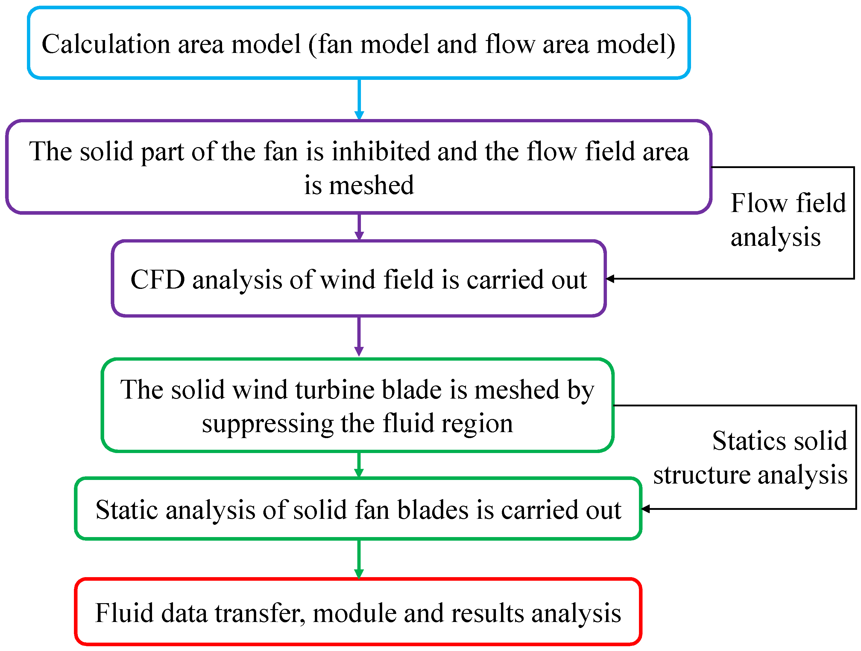
3.1. The Establishment of the Coupling Model

In the simulation, the calculation area is selected as 30 × 20 × 15 m. The standard Realizable k-epsilon turbulence model is used due to the large computational load, along with the SIMPLE algorithm to ensure faster convergence. At the same time, by selecting the Enhance Wall Treatment option, the simulation errors can be reduced, and the fluid characteristics typically avoided near the blade can be captured.

In this model, analysis models of four kinds of leaves are established simultaneously in the same analysis domain. According to the above analysis, four kinds of blade widths with the highest wind energy utilization coefficient are selected, respectively. The width of three blades is 1.34 m; the width of four blades is 1.0 m; the five-blade blade width is 0.8 m; the six-blade blade width is 0.72 m. The installation Angle is 0°, the wind speed is 8 m/s, and the rotational speed is 20 rpm. The blade surface is set as a non-slip boundary. In the solid computing domain, the hub is set as a fixed-end constraint without considering the gravity load condition. In order to minimize the influence of four wind turbines with different numbers of blades, the distance between them is maintained above 15 m. The figure shows the schematic diagram of the established three-dimensional analysis model.

3.2. Coupled Meshing

For the meshing of the coupling model, the solid region and fluid region need to be distinguished, and grids should be divided respectively for different regions. Meanwhile, an interface is used to connect the interface between fluid and solid [36,37].

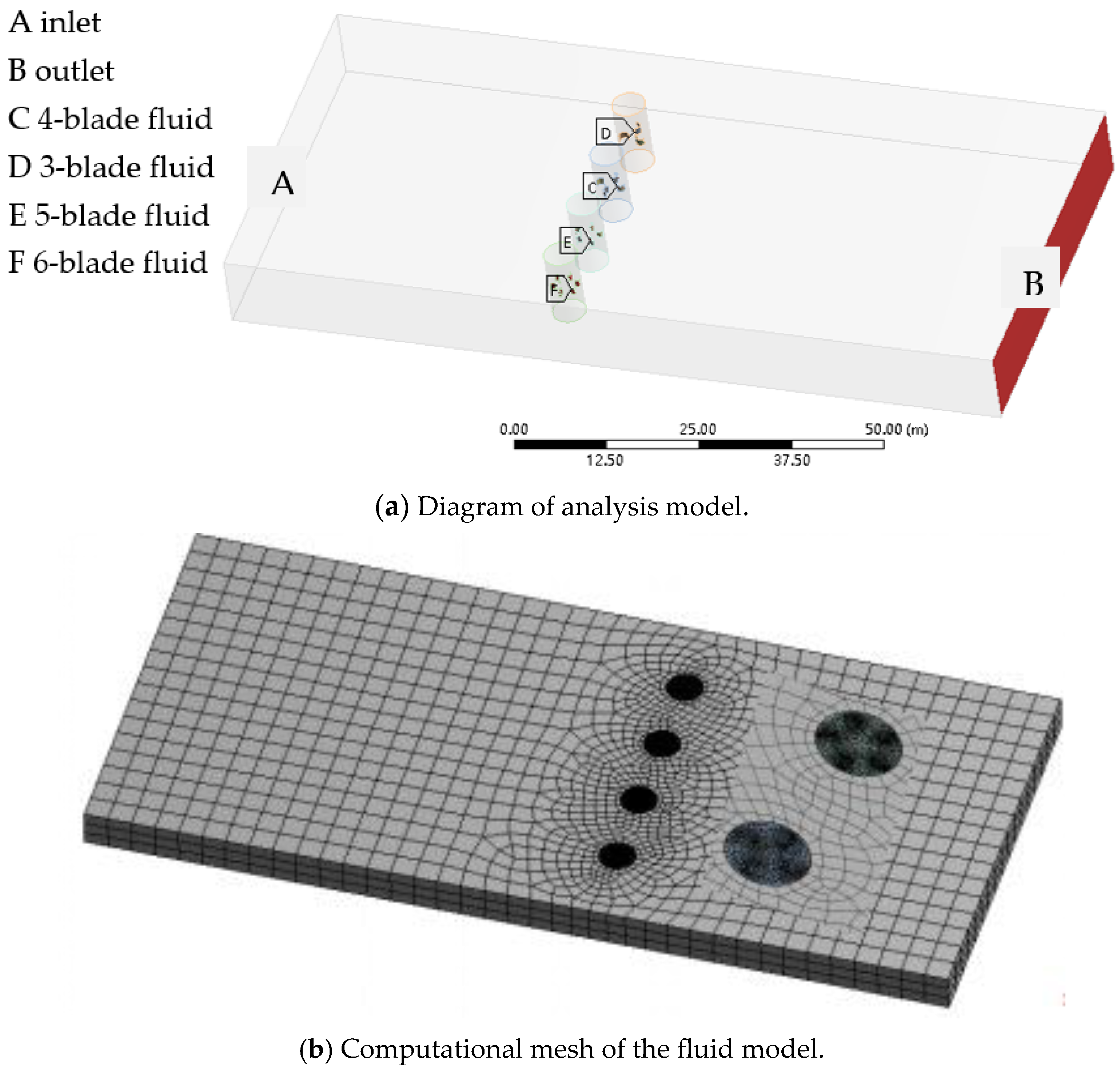
3.2.1. Fluid Meshing

When the flow field is analyzed, the solid wind turbine grid is first suppressed, and a hybrid meshing approach is used to partition the entire domain. In regions near the solid surfaces, an expansion layer is inserted to further capture the effect of the fluid near the wall. Figure 3 shows the division diagram of the fluid grid. Unstructured grids are employed and locally refined in the regions close to the blade rotation area. In contrast, structured grids and a combination of structured and unstructured grids are used in the regions far from the blade rotation area, utilizing a multigrid meshing approach to reduce computational load.

3.2.2. Solid Meshing

For the grid division of the solid region, a combination of tetrahedral and hexahedral meshing techniques is used, with a focus on using tetrahedral meshes and localized treatment of hexahedral meshes. This approach can effectively reflect the blade geometry while minimizing the total number of grids [38,39]. It provides higher computational accuracy and shorter computation time. It is important to note that when partitioning the solid blade, the fluid region needs to be suppressed. Structured grids are employed for meshing the wind turbine blades. Figure 4 shows the solid grid division diagram of a fan blade. In order to compare the difference in the number of blades from the view, we have zoomed out the overall view of the wind turbines with four, five, and six blades. Therefore, from this view, the size and shape of each blade for these four wind turbines seem to be different. However, all parameters of the individual blade are the same for these three-, four-, five-, and six-blade wind turbines.

3.3. Mesh Quality Determination

In order to improve the mesh quality as much as possible, this paper obtains high-quality mesh by means of mesh encryption on the blade surface and nearby boundary area. The quality of the encrypted grid can be seen in Figure 5. It can be seen from the figure that the mesh quality after local mesh encryption is obviously improved, basically reaching more than 0.5. Such a grid satisfies the requirement of the accuracy of simulation results.

3.4. Convergence Judgment

The determination of convergence is very important for the accuracy of the simulation results. During the iterative calculation process, the calculation is considered to have converged when the residual values of each physical quantity reach the specified convergence criteria. By default, FLUENT uses a convergence criterion of reducing the residual values of all variables to 10⁻³, except for the energy residual value [40,41]. The residual curves of the five-blade vertical wind turbine in 40 s were simulated, and it can be seen from Figure 6 that the calculation results have converged at this time. The Y-axis of Figure 6 is the computational residual, which indicates the relative error between the n step and (n + 1) step in the iterative solving process.

3.5. Definition of Physical Parameters

For the linear statics analysis of wind turbines, the material and specific parameters of fan blades need to be considered. Since this paper does not consider heat transfer and other issues, Young’s modulus, Poisson’s ratio, and density are considered when setting parameters of blade material. The thermal expansion coefficient and heat transfer coefficient of the material are not considered. In this paper, the blade of the fan is made of steel, and the specific parameter design is shown in

Table 1. Setting table of blade property parameters.

Poisson’s Ratio	Young’s Modulus	Density	Yield Strength
0.25	206 GPa	7850 kg/m3	2.5 × 108 Pa

[42]:

4. Results and Analysis

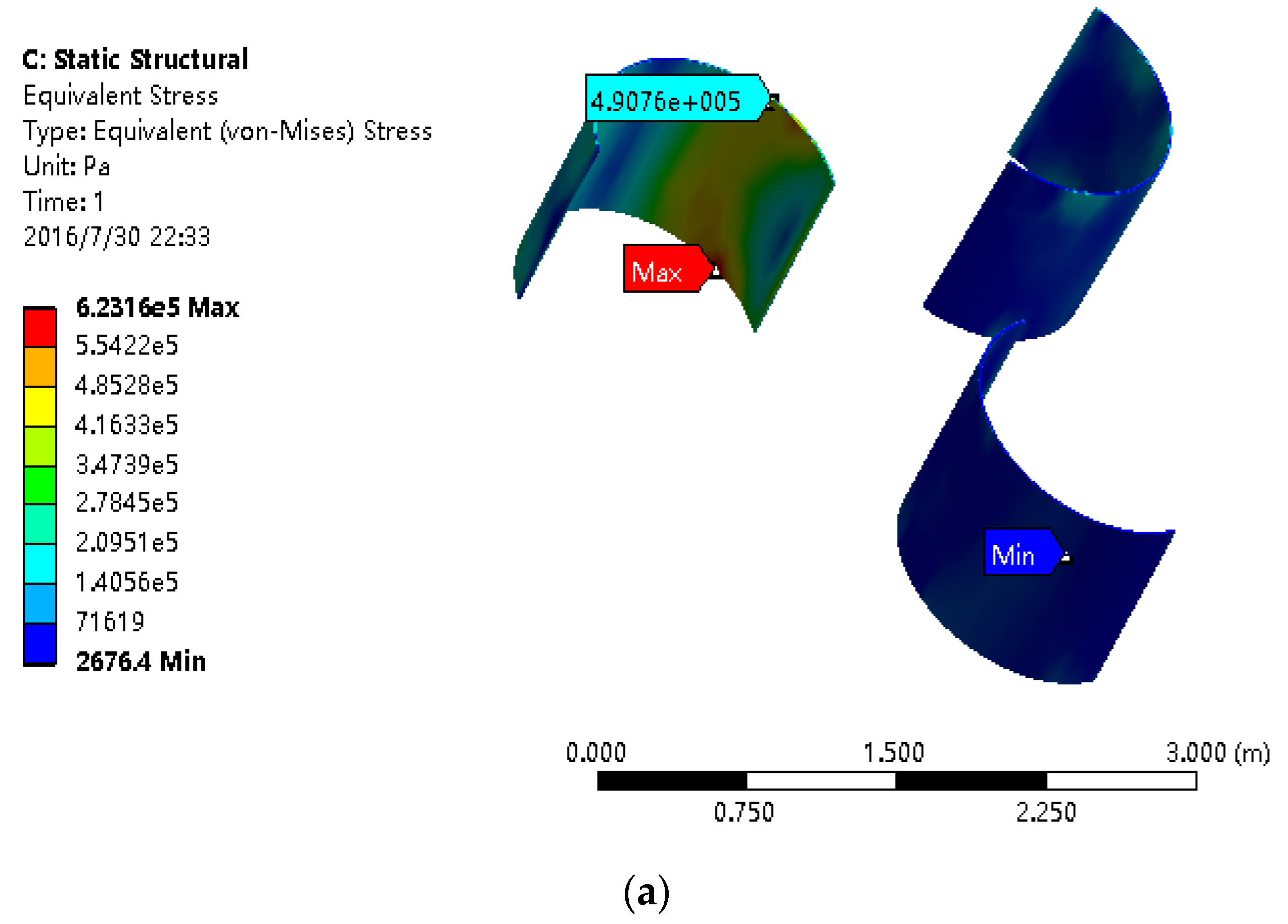
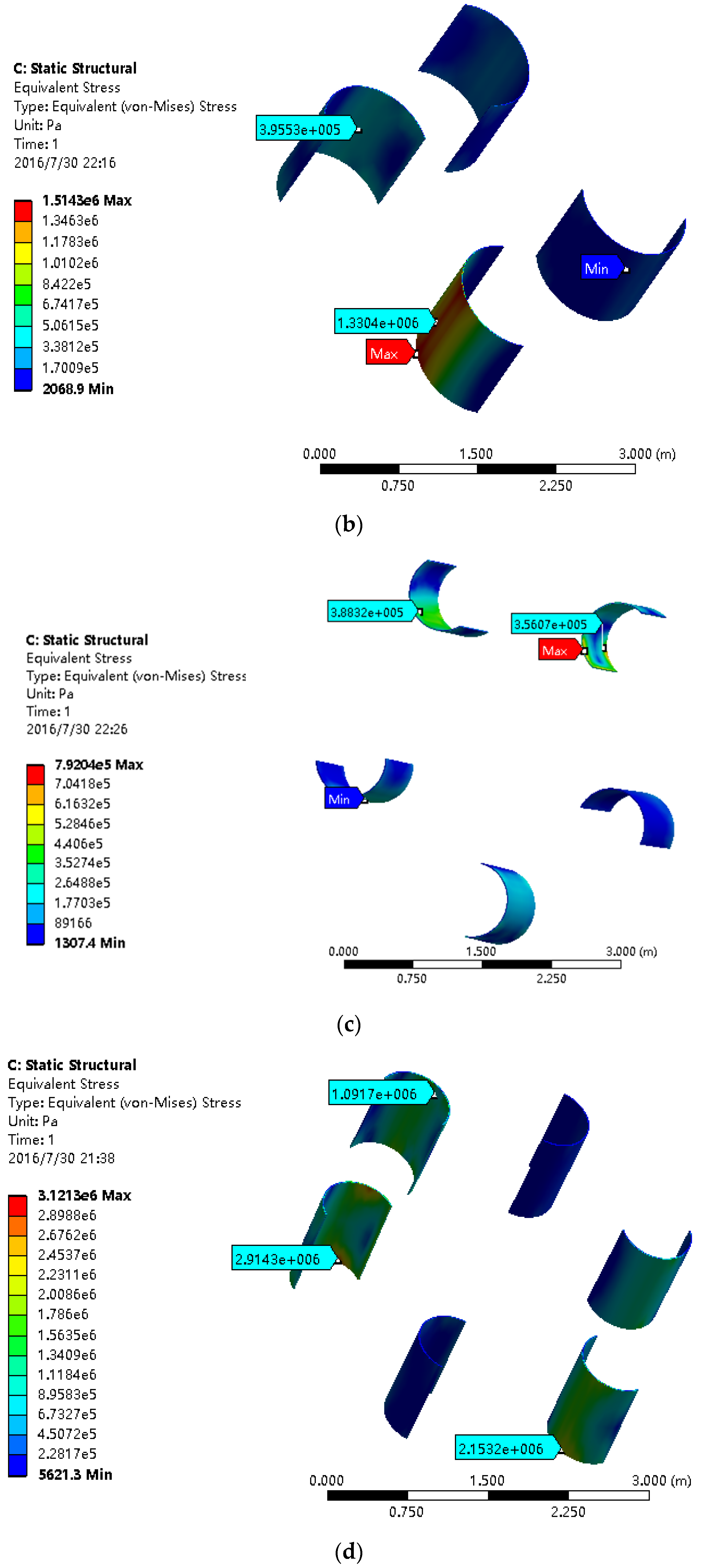
4.1. Structural Stress Analysis

Figure 7 shows the schematic diagram of imported blade pressure. After the pressure data is analyzed, fluent mechanical analysis is carried out using the fluid–structure coupling statics module built. The pressure data generated by the fluid on the fan blade are loaded into the statics analysis module through imported pressure.

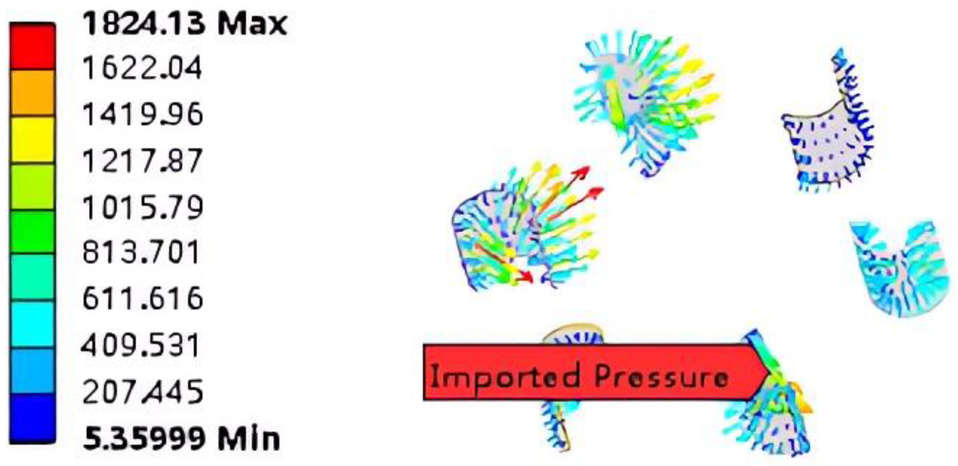
4.2. Pressure Field Analysis

It can be seen from the equivalent pressure field distribution of the blade surface in Figure 8 that, under the same wind speed, the maximum pressure in the overall structure appears in the variable angle position of the blades in the windward region. This is mainly due to the rapid airflow changes, complex turbulence, and significant impact of the wind field on the blade in this region, making the blade prone to bending or damage. Furthermore, it can be found that the equivalent pressure on the surface of four-blade and six-blade wind turbines is significantly higher than that on five-blade and three-blade wind turbines under the same external wind field environment. The maximum equivalent pressure of six blades can be reached at 3.161 × ${10}^6$ Pa. The maximum blade surface pressure of a five-blade wind turbine is 3.5607 × ${10}^5$ Pa.

To analyze the pressure distribution on the blade, the center line of the blade is taken as the reference line to analyze and observe the pressure distribution on the reference line. The simulation diagram is shown in Figure 9.

Table 2. Equivalent pressure gauge at different measuring points of blade.

Fan Type	Point 1	Point 2	Point 3	Point 4	Point 5	Point 6	Point 7	Point 8
three-blade	6.23 × 105	5.76 × 105	4.75 × 105	4.02 × 105	3.62 × 105	3.58 × 105	4.90 × 105	5.01 × 105
four-blade	1.33 × 106	1.38 × 106	1.41 × 106	1.42 × 106	1.41 × 106	1.43 × 106	1.38 × 106	1.37 × 106
five-blade	7.92 × 105	6.61 × 105	4.22 × 105	2.41 × 105	1.61 × 105	1.34 × 105	1.68 × 105	3.93 × 105
six-blade	2.49 × 106	1.80 × 106	1.38 × 106	1.05 × 106	1.15 × 106	1.34 × 106	1.74 × 106	2.63 × 106

shows eight equidistant reference points from top to bottom. Figure 10 shows the pressure distribution trends of different blade reference lines. It can be seen that the pressure of the four-blade and the six-blade is relatively large, and the pressure distribution of the six-blade changes greatly, which can easily cause the deformation of the blade due to uneven pressure distribution. In comparison, the pressure of three blades and five blades is smaller, and the distribution of pressure is more uniform.

As shown in Figure 10 and Table 2, the equivalent pressure distribution curve at different measurement points on the three blades has a gentle trend, and the maximum value is 6.23 × ${10}^5$ Pa, while the minimum value is 3.58 × ${10}^5$ Pa. The distribution curve of the four blades has small local fluctuations, the overall trend is gentle, and the maximum value is 1.43 × ${10}^6$ Pa, while the minimum value is 1.33 × ${10}^6$ Pa. The pressure distribution curve of the five blades decreases slowly at first and then rises slowly with the increase of the measurement point value, and the maximum value is 7.92 × ${10}^5$ Pa, while the minimum value is 1.34 × ${10}^5$ Pa. The pressure distribution curve of the six blades has a sharp trend change, dropping rapidly as the measurement point value increases before rising quickly after reaching the bottom, with a maximum value of 2.63 × ${10}^6$ Pa and a minimum value of 1.05 × 10⁶ Pa.

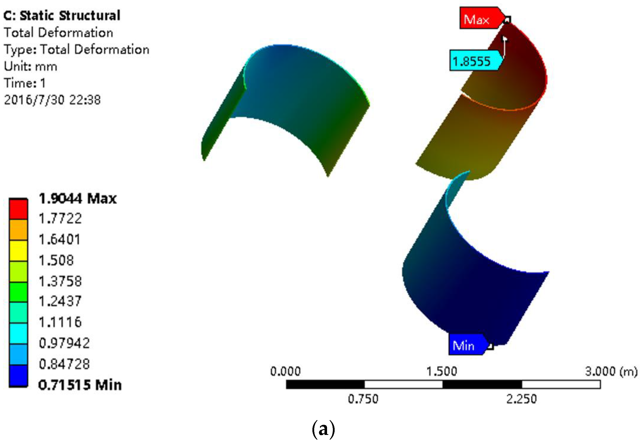
4.3. Deformation Analysis

Figure 11 is the distribution diagram of blade deformation of different wind turbines. From the figure, we can find that the maximum deformation of the three blades is 1.9044 mm, and the minimum value is 0.71515 mm. The maximum deformation of the four blades is 0.84078 mm, with a minimum value of 0.20314 mm. The maximum deformation of the five blades is 2.4217 mm, with a minimum value of 0.12165 mm. The maximum deformation of the six blades is 11.658 mm, with a minimum value of 1.1918 mm. It can be seen from the figure that the maximum deformation of the blade basically appears in the position of the tip and four sides of the blade. At the same time, it can be seen that among the four wind turbine configurations with different blade numbers, the six-blade configuration has the highest maximum deformation, while the four-blade configuration has the lowest maximum deformation.

5. Conclusions

The object studied in this paper is the vertical-axis wind turbine. Considering the different number of wind turbine blades, combined with the aerodynamic theory, the aerodynamic performance of wind turbines is analyzed by computational fluid dynamics (CFD) technology. The FSI method is used to study the pressure exerted on the blade surfaces of three-, four-, five-, and six-blade vertical-axis wind turbines under flow conditions. The results show that:

(1)

For four kinds of wind turbines with different blade numbers, the maximum pressure in the overall structure all appears in the variable angle positions of the blades in the windward region under the same wind speed. This is primarily due to the rapid airflow changes, complex turbulence, and significant influence of the wind field on the blades at these positions, making them prone to bending or damage;

(2)

The equivalent pressure on the surface of four-blade and six-blade wind turbines is significantly higher than that of five-blade and three-blade wind turbines under the same external wind field environment. The equivalent pressure distribution curves at different measurement points on the three blades exhibit a gentle trend. The four-blade distribution curve shows minor fluctuations in localized areas but has an overall gentle trend. The pressure distribution curve of the five blades decreases slowly at first and then rises slowly with the increase of the measurement point value. The pressure distribution curve of the six blades has a drastic change, rapidly decreasing as the measurement points increase, reaching the lowest point, and then quickly rising;

(3)

The maximum deformation of the blades primarily occurs at the blade tips and edges. Additionally, among the four-wind turbine configurations with different blade numbers, the six-blade configuration has the highest maximum deformation, while the four-blade configuration has the lowest maximum deformation.

The numerical results obtained in the present study could provide theoretical guidance for designing and optimizing vertical-axis wind turbines.

References

1. Wang, F.; Xu, X.Y. Prospect and problems of wind power market in China. Power Stat. Aux. Equip. 2010, 31, 1–4. [Google Scholar]
2. Li, Y.; Yang, S.B.; Feng, F.; Kotar, T. A review on numerical simulation based on CFD technology of aerodynamic characteristics of straight-bladed vertical axis wind turbines. Energy Rep. 2023, 9, 4360–4379. [Google Scholar] [CrossRef]
3. Ma, Y.H.; Zhang, Y.C.; Zhang, C.Y.; Guo, M.J.; Chen, J.Y.; Zhang, H.Y.; Liu, S.R. A review and consideration of wind energy utilization efficiency research. Environ. Technol. Innov. 2022, 12, 179–181. [Google Scholar]
4. Lin, Y.X.; Zhang, J.Y. Development status and prospect of offshore wind power. Distrib. Energy 2023, 8, 1–10. [Google Scholar]
5. Li, Z.; He, D. Reviews of fluid dynamics researches in wind energy engineering. Adv. Mech. 2013, 43, 472–525. [Google Scholar]
6. Zhang, L.; Ye, T.; Xin, Y.; Han, F.; Fan, G. Problems and Measures of Power Grid Accommodating Large Scale Wind Power. Proc. CSEE 2010, 30, 1–9. [Google Scholar]
7. Al-Ghriybah, M.; Zulkafli, M.F.; Didane, D.H.; Mohd, S. The effect of spacing between inner blades on the performance of the Savonius wind turbine. Sustain. Energy Tech. 2021, 43, 100988. [Google Scholar] [CrossRef]
8. Zhang, Z.H.; Muhammad, A.; Liu, Q. New Theory and Method for Improving Utilization and Conversion Rate of Wind Turbine:Establishment of Blade Outlet Angle Formula and Its Application. J. Basic Microbiol. 2017, 25, 1040–1047. [Google Scholar]
9. Yu, D.; Wang, K.Y.; Liu, H.X.; Ding, H.Q.; Kong, F.K.; Liu, W.Q. Numerical Simulation of Energy Capture Efficiency of a Vertical Axis Turbine Under Complex Sea Conditions. Mar. Technpl. Soc. J. 2021, 55, 17–28. [Google Scholar] [CrossRef]
10. Wang, J.; Ren, P.L.; Wang, X.S. CFD study of a new type of vertical axis wind turbine. J. Eng. Thermophys. Rus. 2012, 33, 63–66. [Google Scholar]
11. Yang, Y.F.; Pan, W.; Zhu, H.Q. An Overview and Recent Research Progresses of Vertical Axis Wind Turbine. China Mech. Eng. 2013, 24, 703–709. [Google Scholar]
12. Ai, C.; Zhang, Y.B.; Jia, C.D.; Zhang, L.; Kong, X.D. Research on rotating speed control of the vertical axis hydraulic wind turbine. T Can. Soc. Mech. Eng. 2020, 44, 567–579. [Google Scholar] [CrossRef]
13. Boztas, A.; Demirbas, O.; Sahin, M. Investigation of vertical axis wind turbines and their components design. Turk. J. Electromec. Energy 2021, 6, 64–72. [Google Scholar]
14. Ma, L.J.; Chen, J.; Du, G.; Cao, R.J. Numerical simulation of aerodynammic performance for wind turbine airfoils. Acta Energ. Sol. Sin. 2010, 31, 203–209. [Google Scholar]
15. Kirke, B. Evaluation of Self-Starting Vertical Axis Wind Turbines for Stand-Alone Applications. Doctoral Dissertation, Griffith University, Gold Coast, QLD, Australia, 1998. [Google Scholar]
16. Hoogedoom, E.; Jacobs, G.B.; Beyene, A. Aero-elastic behavior of a flexible blade for wind turbine application: A 2D computational study. Energy 2010, 35, 778–785. [Google Scholar] [CrossRef]
17. MacPhee, D.W.; Beyene, A. Fluid–structure interaction analysis of a morphing vertical axis wind turbine—ScienceDirect. J. Fluid. Struct. 2016, 60, 143–159. [Google Scholar] [CrossRef]
18. Hsu, M.C.; Bazilevs, Y. Fluid-structure interaction modeling of wind turbines: Simulating the full machine. Comput. Mech. 2012, 50, 821–833. [Google Scholar] [CrossRef]
19. Han, Z. Fluid-Solid Coupling Analysis of Blades of Small Vertical Axis Wind Turbines. Master’s Thesis, Inner Mongolia University of Technology, Hohhot, China, 2021. [Google Scholar]
20. Wei, K.P. Research on Unsteady Fluid Solid Coupling Numerical Simulation Method of H-Type Vertical Axis Wind Turbine. Master’s Thesis, Guangdong University of Technology, Guangdong, China, 2020. [Google Scholar]
21. Feng, F.; Li, Y.; Chen, L.X.; Tian, W.Q.; Zhang, Y.W. A simulation and experimental researach on aerodynamic characteristics of combined type vertical axis wind turbine. Acta Energiae Solaris Sin. 2014, 35, 855–860. [Google Scholar]
22. Ageze, M.B.; Hu, Y.F.; Wu, H.C. Comparative Study on Uni- and Bi-Directional Fluid Structure Coupling of Wind Turbine Blades. Energies 2017, 10, 1449. [Google Scholar] [CrossRef] [Green Version]
23. Liao, M.F.; Li, Y.; Wang, Q.Y.; Lu, P. Study on Fluid-structure Interaction Characteristic for Large Scaled Wind Turbine Blade. Mech. Sci. Technol. Aerosp. Eng. 2018, 37, 493–500. [Google Scholar]
24. Zhang, Z.Y.; Wang, T.G.; Chen, L.; Xu, B.F.; Luo, Y. Aerodynamic design and numerical optimization for conceptual wind turbine blades with multiple winglets. Acta Aerodyn. Sin. 2013, 31, 127–131. [Google Scholar]
25. Zheng, J.H.; Cui, D.; Jiang, P.X. Static analysis of MW wind turbine nacelle chassis. Mach. Des. Manuf. 2010, 11, 197–198. [Google Scholar]
26. Marsh, G. Wind turbines: How big can they get? Refocus 2005, 6, 22–28. [Google Scholar] [CrossRef]
27. Yang, C.X.; Li, S.F. Study of post-stalled airfoil of a H-type vertical axis wind turbine. J. Lanzhou Univ. Technol. 2015, 41, 51–54. [Google Scholar]
28. Duque, E.; Burkland, M.; Johnson, W. Navier-Stokes and Comprehensive Analysis Performance Predictions of the NREL Phase VI Experiment. J. Sol. Energy Eng. 2003, 125, 43–61. [Google Scholar] [CrossRef]
29. Versteeg, H.K.; Malalasekera, W. An Introduction to Computational Fluid Dynamics: The Finite Volume Method; World Book Inc.: London, UK, 2010. [Google Scholar]
30. Yang, S.M.; Tao, W.S. Heat Transfer Theory, 4th ed.; Beijing Higher Education Press: Beijing, China, 2006. [Google Scholar]
31. Hirsch, C. Numerical Computation of Internal and External Flows. Int. J. Heat Fluid F. 2007, 10, 371. [Google Scholar]
32. Mirzaei, M.; Ardekani, M.A.; Doosttalab, M. Numerical and experimental study of flow field characteristics of an iced airfoil. Aerosp. Sci. Technol. 2009, 13, 267–276. [Google Scholar] [CrossRef]
33. Tang, J.P. Ansys Fluent 16.0 Super Learning Manual; People’s Post and Telecommunications Publishing House: Beijing, China, 2016. [Google Scholar]
34. Fu, P.; Farzaneh, M. A CFD approach for modeling the rime-ice accretion process on a horizontal-axis wind turbine. J. Wind Eng. Ind. Aerod. 2010, 98, 181–188. [Google Scholar] [CrossRef]
35. Kong, C.; Bang, J.; Sugiyama, Y. Structural investigation of composite wind turbine blade considering various load cases and fatigue life. Energy 2005, 30, 2101–2114. [Google Scholar] [CrossRef]
36. Yang, J.; Wu, M.P.; Ye, J.Y.; Wang, Y. Aerodynamic Design and Strutural Studies of Wind Turbine Blades. Machinery 2014, 52, 5–8. [Google Scholar]
37. Liu, P.F.; Liu, J.W.; Wang, C.Z. Finite element analysis of damage mechanisms of composite wind turbine blade by considering fluid/solid interaction. Part II: T-shape adhesive structure. Compos. Struct. 2022, 301, 116212. [Google Scholar] [CrossRef]
38. Gao, Y.D.; Hu, X.; Duo, C. Concrete Truck Mixer Blade Fatigue Analysis Based on the Fluid-Structure Interaction. Mach. Des. Manuf. 2015, 291, 47–49. [Google Scholar]
39. Ding, Y.; Wu, J.H. ANSYS CFX14.0 from Beginner to Master; Beijing Tsinghua University Press: Beijing, China, 2013. [Google Scholar]
40. Cao, W.B.; Li, H.X.; Gao, H.H. Convergence analysis and application of the slip boundary conditions. J. Natl. Def. Univ. Sci. Technol. 2013, 35, 12–18. [Google Scholar]
41. Chong, X. Assessment of second-order velocity-slip boundary conditions of the navier-stokes equations. J. Sol. Energy Eng. 2007, 39, 1–6. [Google Scholar]
42. Lv, C. Study of Dynamic Grid Deformationical Algorithm and Its Application. Master’s Thesis, National University of Defense Technology, Changsha, China, 2010. [Google Scholar]
Figure 1. Graphical abstract of this paper.
Applsci 13 08612 g001
Figure 2. Process of fluid-solid coupling analysis.
Applsci 13 08612 g002
Figure 3. Physical model and computational mesh.
Applsci 13 08612 g003
Figure 4. Models of solid wind turbine, (a) three-blade, (b) four-blade, (c) five-blade, and (d) six-blade.
Applsci 13 08612 g004
Figure 5. Grid quality display.
Applsci 13 08612 g005
Figure 6. Residual curve diagram of wind turbine running in model 40 s.
Applsci 13 08612 g006
Figure 7. Import pressure of the blades.
Applsci 13 08612 g007
Figure 8. Vane variable distribution map of different wind turbines: (a) three blades; (b) four blades; (c) five blades; (d) six blades.
Applsci 13 08612 g008aApplsci 13 08612 g008b
Figure 9. Leaf reference line schematic diagram.
Applsci 13 08612 g009
Figure 10. Trend map of stress distribution of different blade reference lines.
Applsci 13 08612 g010
Figure 11. Vane deformation map of different wind turbines: (a) three blades; (b) four blades; (c) five blades; (d) six blades.
Applsci 13 08612 g011aApplsci 13 08612 g011b