Sensitivity of Modern Deep Learning Neural Networks to Unbalanced Datasets in Multiclass Classification Problems

Featured Application

The results of the work can be used in computer vision systems for medical problems, or other applications where the training data is highly imbalanced.

Abstract

One of the critical problems in multiclass classification tasks is the imbalance of the dataset. This is especially true when using contemporary pre-trained neural networks, where the last layers of the neural network are retrained. Therefore, large datasets with highly unbalanced classes are not good for models’ training since the use of such a dataset leads to overfitting and, accordingly, poor metrics on test and validation datasets. In this paper, the sensitivity to a dataset imbalance of Xception, ViT-384, ViT-224, VGG19, ResNet34, ResNet50, ResNet101, Inception_v3, DenseNet201, DenseNet161, DeIT was studied using a highly imbalanced dataset of 20,971 images sorted into 7 classes. It is shown that the best metrics were obtained when using a cropped dataset with augmentation of missing images in classes up to 15% of the initial number. So, the metrics can be increased by 2–6% compared to the metrics of the models on the initial unbalanced data set. Moreover, the metrics of the rare classes’ classification also improved significantly–the True Positive value can be increased by 0.3 or more. As a result, the best approach to train considered networks on an initially unbalanced dataset was formulated.

1. Introduction

The multiclass classification problem is one of the most common and important tasks in modern machines and deep learning applications in various fields [1,2,3,4,5]. One such area is medicine, where the solution to such problems allows for improving the systems of diagnostics, rehabilitation, and the life quality support of patients. Currently, there are numerous works devoted to using neural networks for solving classification problems in medicine.

For example, the classification of cancer on pathological images of cervical tissues using deep learning algorithms was considered by Pan Huang, et al. in [6]. The authors used ResNet50 [7], DenseNet12, Inception_v3 [8], and VGGNet19 [9] for an almost balanced dataset consisting of 468 RGB images, including 150 images of the norm, 85 low-grade squamous intraepithelial lesions images, and 104 images of high-grade squamous intraepithelial lesions. Swaraj and Verma [10] solved the COVID-19 classification problem on chest X-ray images. The dataset consisted of 15,371 posterior-to-anterior chest X-ray images. The authors used LeNet [11], VGG-16 [12], ResNet-50, AlexNet [13], Xception [14] and Inception_v3 architectures as deep learning models for training. As a result, LeNet showed an accuracy of 74.75% on a validation dataset, AlexNet—70.04%, ResNet-50—75.71%, VGG-16—87.34%, Inception_v3—84.29%, Xception—67.76%. State of art algorithms are also used for solving actual medical problems. For example, works [15,16] provide an overview of the application of transformers models for solving various medical problems related to the analysis of medical images. The types of problems that can be solved by transformer models, their architecture, and metrics were considered. 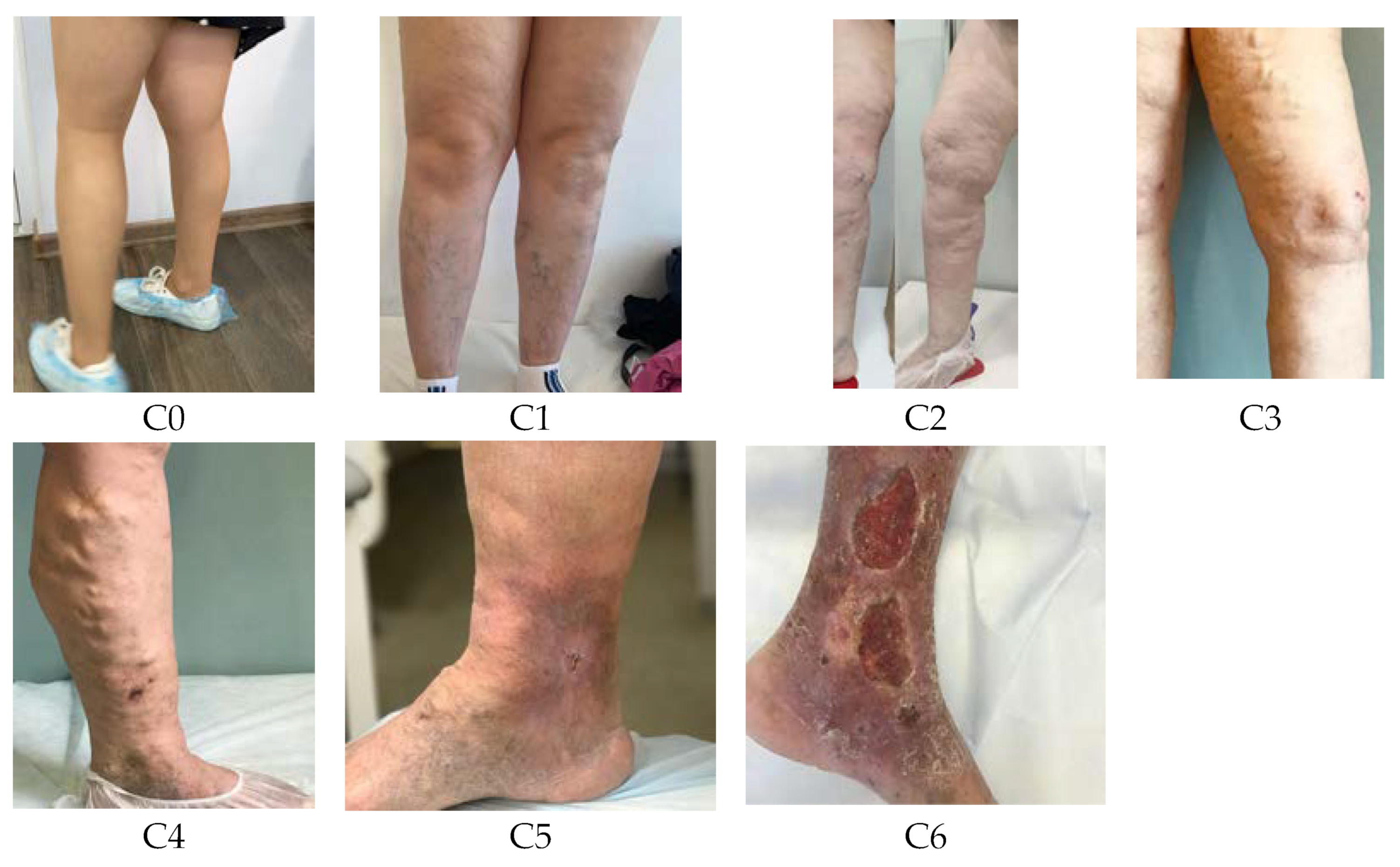The paper [17] states the approach of applying transformers to solving the problem of classifying medical images of the stage of chronic venous disease for self-diagnosis of a patient by using the image of the patient’s legs.

Deep learning algorithms are used to solve classification problems in other areas of science and technology too. Gangsar and Tiwari [18] studied vibration and current monitoring for effective fault prediction in an induction motor by using multiclass support vector machine (MSVM) algorithms. Ceyhan et al. [19] shared the results of experiments aimed at classifying wheat varieties using deep learning methods, which made it possible to create an original approach for such classification, which can be used in industry, including on equipment with low memory/small computing power.

Despite the widespread use of deep learning methods, their training faces several challenges. Therefore, one of the critical problems in multiclass classification tasks is the imbalance of the dataset. This is especially important when using contemporary pre-trained neural networks which were mentioned before, where the last layers of the neural network are retrained. With an unbalanced dataset, the error of relating an object to the correct class increases, which cannot always be eliminated by changing the training parameters of a neural network.

Note that most of the data obtained in solving practical problems are not balanced. This is due to the nature of such problems. For example, most medical datasets are imbalanced because the distribution of patients according to the stages of the disease is uneven. Moreover, the distribution of the disease stages of those who sought medical help is also uneven. The number of correct banking transactions will always be significantly greater than the number of fraudulent transactions. There are more distinct types of civilian vehicles than special ones. The distribution of images of different animals that we can use for classification is also not uniform. There will be more images of domestic animals than images of rare or wild animals.

There are a number of works devoted to various techniques for increasing the metrics of training models on an unbalanced dataset. A feasible way to improve the quality of the classification is to change the number of objects in the dataset by data augmentation, data mining, etc. It is commonly said that data augmentation can increase the values of training metrics.

The authors of article [20] propose the modified VGG16 model for the classification of pneumonia X-ray images. The presented IVGG13 model trained on an augmented dataset produced good metrics with the F1-measure compared with the best convolutional neural networks for medical image recognition. At a time when COVID-19 was the most common in the world, Jain et al. [21] presented an approach to form a classifier neural network for COVID-19 diagnoses by X-ray images. This approach contained 4 phases including data augmentation. As shown in [22], the strategy of training used with data augmentation techniques that avoid overfitting problems on ConvNets shows the best results.

Song et al. [23] used BLogitBoost-J, LogitBoost [24], and BABoost [25] methods for multiclass classification on imbalanced datasets of Thyroid and Glass from the UCI data repository. Both datasets contained only numerical (non-images) samples. The thyroid dataset had 3 classes and the sample quantity for each class was 168:368:6666. The glass dataset consisted of 6 types. The ratio of the sample quantity was 70:76:17:13:9:29. LogitBoost algorithm, extended from Adaboost, is an adaptive algorithm that can acquire higher prediction precision. Because it is based on conditional Bernoulli likelihood without prior probability in consideration, the LogitBoost algorithm will lead to a high minority class prediction error. Song et al. [25] propose an improved BLogitBoost, based on a stratified normalization method, to deduce the badness of LogitBoost in the case of two-class unbalanced data. The authors proposed a new algorithm named BLogitboost-J. The BABoost, in turn, was also an improved AdaBoost algorithm for unbalanced classification data. The difference is that in each round of boosting, the BABoost algorithm assigns more weights to the misclassified examples in the minority class by a user-specified parameter.

Bhadra et al. in [26] classified three different environmental chemical stimuli, using fifteen statistical features, extracted from the plant electrical signals. They used the imbalanced dataset consisting of 37,834 data blocks for three chemical stimuli. The ratio was 628:1488:35718. The authors applied Monte Carlo under-sampling of major classes and they used eight algorithms (AdaBoost, Decision tree, Gaussian Naive Bayes, k-nearest Neighbors, Multilayer perceptron classifier, Quadratic discriminant analysis, Random Forest, and Support vector machine) to compare their performance.

Nurrahman et al. [27] solved multiclass classification anemia and iron deficiency using the XGBoost method. The data set consisted of 11,327 samples into 4 categories. The sample ratio was as follows: iron deficiency anemia—9.40%; iron deficiency—14.95%; Anemia—11.93%; Normal—63.72%. The data preprocessing included MissForest imputation (a method for filling gaps in data), feature selection using the Boruta method, and feature generation using SMOTE. Then they applied the XGBoost classification algorithm.

Meisen and Kraus [28] compare several approaches to deal with the problem of unbalanced sidescan sonar datasets for classification tasks. They used the imbalanced dataset consisting of 1290 images for 3 classes. The ratio was 30:630:630. This data was labeled, normalized, and prepared for use by neural networks. In this paper, they have introduced a new method of transfer learning for GANs on sidescan sonar data named TransfGAN which uses ray-traced images for pre-training. On their sidescan sonar image dataset augmentation with synthetic images from TransfGAN increases the balanced accuracy by more than 10% while also achieving a 3% higher macro F1 score.

Bhowan et al. in [29] compared the effectiveness of two genetic programming classification strategies. The first uses the standard (zero) class-threshold, while the second uses the “best” class-threshold determined dynamically on a solution-by-solution basis during evolution. The authors conducted experiments for five benchmark binary classification problems on datasets from the UCI Repository of Machine Learning Databases, and the Intelligent Systems Lab at the University of Amsterdam. One of the five datasets used for the experiment contained 267 records derived from cardiac Single Photon Emission Computed Tomography (Spect) images. There are 55 “abnormal” records (20.6%) and 212 “normal” records (79.4%), an imbalance ratio of approximately 1:4. Study results suggest that there is no overall difference between the two strategies and that both strategies can evolve good solutions in binary classification when used in combination with an effective fitness function.

At the same time, data mining usage can also have a positive impact on the performance of neural networks. In ref. [30] various approaches to medical data mining were considered, as well as the learning outcomes after applying each of the approaches. It also showed that all considered mining methods increase the accuracy of the neural networks. Bellazzi and Zupan [31] stated that many data mining methods can be successfully applied to a variety of practical problems in clinical medicine and are an excellent means of increasing network performance for medical data processing tasks.

So, most of the work either uses different data-filling techniques and different boosting algorithms. One more approach is to use implicit ways to replicate the smaller class until you have as many samples as in the larger one, for example, class weight for some neural network models. However, this way cannot be considered as acceptable for computer vision tasks.

For binary classification problems, cost-sensitive learning can be used. However, this approach is too difficult to generalize for multiclass classifications.

Various ensemble methods can also be used to solve problems of multiclass image classification. However, the result of their application strongly depends on the problem being solved and the dataset used.

The dataset imbalance affects the training results of each neural network (NN) differently, as does data preprocessing similar to data augmentation and data mining. It is also the subject of interest to study which of the methods or their combinations for reducing the imbalance of a dataset is most preferable for a particular neural network.

The aim of the work was to compare the results of using contemporary neural networks for multiclass classification on a highly imbalanced image dataset and to formulate an approach for normalizing such datasets to improve the quality of a deep neural network (DNN) model training.

To achieve this goal, we studied the sensitivity to a dataset imbalance of the following contemporary neural networks: Xception, ViT-384 [32], ViT-224, VGG19, ResNet34 [33], ResNet50, ResNet101 [34], Inception_v3, DenseNet201 [35], DenseNet161 [36], and DeIT [37]. Different imbalance reduction techniques and their ensembles were used to determine this sensitivity. Based on the analysis of the obtained learning metrics, recommendations were formulated on the use of the ensemble method for dataset normalization.

The remainder of this paper is organized as follows. The data processing methods, data mining ways, as well as trained neural networks are described in Section 2. The performance evaluation and research results are stated in Section 3. The validation of the suggested approach is in Section 4. Finally, Section 5 discusses the study’s findings, results, and the main conclusion of the work.

2. Materials and Methods

2.1. Datasets

The study was carried out in three stages. The models’ parameters were the same for all stages. At the first stage, all the following neural networks Xception, ViT-384, ViT-224, VGG19, ResNet34, ResNet50, ResNet101, Inception_v3, DenseNet201, DenseNet161, DeIT were trained on the full dataset. The dataset was an unbalanced set of 20,971 leg images distributed across 7 classes (C0, C1, …, C6) according to the CEAP classification for chronic venous diseases [17]. Samples from the dataset are shown in Figure 1. The only image preprocessing was resizing to 224 × 224 px.

The distribution of images by classes was as follows: C0—12%; C1—26%; C2—14%; C3—33%; C4—11%; C5 and C6 classes—2% each as shown in Figure 2 and

Table 1. Class distribution of images of the initial dataset.

Class	C0	C1	C2	C3	C4	C5	C6
Number of images	2494	5495	2861	6850	2386	458	427

.

As can be seen in Figure 2, the initial dataset was significantly unbalanced. The number of classes C5 and C6 are extremely small compared to other classes, and class C3 is dominant.

In the second stage, small datasets were used. Cutting off the dataset by the smallest class is a good approach to avoid unbalanced, when the original dataset is big enough. To form small but balanced datasets, the initial dataset was cut off by the smallest class (C6). The excluded images were used as a validation dataset. To avoid randomness in the result obtained, three datasets were formed, where classes C0-C5 contained, if possible, different images. So, we constructed three datasets—“small_ds_1”, “small_ds_2”, “small_ds_3”. The distribution of images by classes is shown in

Table 2. Class distribution of images of the small datasets.

Class	C0	C1	C2	C3	C4	C5	C6
small_ds_1	455	448	480	442	454	430	414
small_ds_2	444	452	432	455	435	458	427
small_ds_3	448	450	432	453	435	458	427

.

At the third stage, the dataset was formed as follows. Each class was cropped to the number of images equal to the size of class C6 + 15% of it. Then the missing images in classes C5 and C6 were augmented. Such an approach can help generate new samples from existing samples using standard image conversion algorithms. It is based on deep learning concepts where a slightly modified original image is considered as a new image.

However, a large amount of artificial data can be detrimental to the ability of a machine learning model to generalize. Therefore, misapplication of this approach can lead to overfitting. That is why we augmented the dataset by not more than 15%. The distribution of images by classes for “aug_ds” is shown in Table 3.

We used the following image transform algorithms for data augmentation:

• Shift Scale Rotate. Randomly apply affine transforms: translate, scale, and rotate images. The parameters were as follows:

  -

  The scaling factor range was (−0.5, 0.5). So, an image was randomly zoomed out or in of the original size to any percent in this range.

  -

  Shift factor ranges for both height and width were (−0.05, 0.05).

  -

  Rotation range was (−30, 30).

  -

  The probability of applying this transform was set to 0.6.

• Random Crop. Crop random parts of the images with fixing size. The height and width of the crop were 224 px.
• Horizontal Flip. Flip an image 180 degrees to obtain a mirror image. The probability of applying this transform was set to 0.5.
• RGB Shift. Randomly shift values for each Red-Green-Blue channel of an image. The range for changing values for the red channel. Ranges for changing values for all channels were (−15, 15). The probability of applying this transform was 0.6.
• Random Brightness Contrast. Randomly change the brightness and contrast of an image. The probability of applying this transform was set to 0.7.

Table 3. Class distribution of images of the cropped and augmented dataset.

Class	C0	C1	C2	C3	C4	C5	C6
aug_ds	518	504	506	498	425	518	498

Table 3. Class distribution of images of the cropped and augmented dataset.

Class	C0	C1	C2	C3	C4	C5	C6
aug_ds	518	504	506	498	425	518	498

The distribution of samples for all obtained datasets are shown in Figure 3.

2.2. Deep Learning Neural Networks

We trained the following 11 different contemporary architectures of deep learning neural networks on the obtained datasets: ResNet34, ResNet50, ResNet101, VIT-base-patch16-224, VIT-base-patch16-384, DeIT-base-patch16-224, DenseNet161, DenseNet201, VGG19, Inception, Xception. Our goal was to formulate the best approach to train these networks on an initially unbalanced dataset.

ResNet (Residual Neural Network) models are the most popular fully convolution models in computer vision. ResNet is a deep learning model in which the weight layers learn residual functions with reference to the layer inputs. The fundamental difference between ResNet and classical convolutional neural networks is shortcut connections. Thanks to them, ResNet can contain a large number of layers while bypassing the vanishing gradient problem, which helps to catch more features from input images. In the work, we used ResNet34, ResNet50, and ResNet101 models. In general, the ResNet models consist of residual blocks (Figure 4a). Some ResNet models (for ex. ResNet50 and ResNet101) have the Bottleneck block (Figure 4b).

Visual image transformer (VIT) and Data efficient image transformer (DeIT) are the newest architecture in computer vision at this moment. They are based on transformer architecture, which was created for natural language processing tasks. The main idea of these architectures is to use not pixels as layers, but fixed-size image pieces called tokens or patches. These tokens process similar to text tokens on NLP, using attention layers for obtaining image embeddings. DeIT can be considered as a VIT model with an additional distillation token. The architecture of ViT transformer neural networks is shown in Figure 5.

DenseNet is modified ResNet. DenseNet establishes a dense connection between all the front and back layers. Another important feature of DenseNet is the implementation of feature reuse via feature bonding on a channel. These features allow DenseNet to achieve higher performance than ResNet with fewer parameters and computational overhead. The Basic DenseNet Composition Layer block consists of a pre-activated batch normalization layer, ReLU activation function, and a 3 × 3 convolution layer. Multiple Dense Blocks with Transition Layers are shown in Figure 6.

VGG architecture (Figure 7) is one of the first convolution neural networks models. Its main idea is to learn by parts. This is achieved by adding new layers to the old frozen layers and training model.

The ideas behind Inception were first created by Google in their GoogLeNet model. This model was based on inception blocks, which parallel apply on a previous layer different convolution filters and then concatenate results. The authors of Inception changed the kernel size and the number of convolutional filters, which made it possible to reduce the number of blocks and size of the model. The Inception block is shown in Figure 8.

Xception is an upgrade of Inception based on xception blocks. Unlike the inception block, it applies a 1 × 1 convolution to the previous layer, splits it into channels, and applies its own convolution filter with the same kernel size to each (Figure 9). This mechanism allows the network to be even more compact and give better results.

2.3. Training Procedure

Dataset preprocessing included only resizing of input images to 224 × 224 px. For VIT-base-patch16-384 the input images were resized to 384 × 384 px. The constructed datasets were divided into training (80%) and test (20%) datasets.

The training environment was CPU AMD Ryzen 5 5600 GPU NVIDIA RTX 2070 Super RAM 16 GB.

The training parameters for all models are shown in

Table 4. The training parameters for all considered models.

	Number of Parameters	Image Size	Batch Size	Number of Hidden Layers	Optimizer	Learning Rate
ResNet34	21,797,672	224	64	34	Adam	1 × 10−4
ResNet50	25,557,032	224	64	50	Adam	1 × 10−4
ResNet101	44,549,160	224	64	101	Adam	1 × 10−4
VGG19	143,667,240	224	16	19	Adam	1 × 10−4
DenseNet161	28,681,000	224	8	161	Adam	1 × 10−4
DenseNet201	20,013,928	224	8	201	Adam	1 × 10−4
Inception_v3	27,161,264	224	16	48	Adam	1 × 10−4
Xception	22,855,952	224	8	71	Adam	1 × 10−4
VIT-base-patch16-224	86,418,432	224	32	12	AdamW	5 × 10−5
DeIT-base-patch16-224	86,418,432	224	32	12	AdamW	5 × 10−5
VIT-base-patch16-384	86,900,000	384	2	12	AdamW	5 × 10−5

. The rest of the parameters had default values.

2.4. Metrics

To evaluate the quality of model training we used the following metrics—Accuracy, Precision, Recall, F1, True Positive Rated, True Negative Rated, False Positive Rated, False Negative Rated.

Accuracy measures the number of correct predictions made by a model in relation to the total number of predictions made:

$$\mathrm{A}\mathrm{c}\mathrm{c}\mathrm{u}\mathrm{r}\mathrm{a}\mathrm{c}\mathrm{y}=\frac{\mathrm{C}\mathrm{o}\mathrm{r}\mathrm{r}\mathrm{e}\mathrm{c}\mathrm{t} \mathrm{c}\mathrm{l}\mathrm{a}\mathrm{s}\mathrm{s}\mathrm{i}\mathrm{f}\mathrm{i}\mathrm{c}\mathrm{a}\mathrm{t}\mathrm{i}\mathrm{o}\mathrm{n}}{\mathrm{A}\mathrm{l}\mathrm{l} \mathrm{c}\mathrm{l}\mathrm{a}\mathrm{s}\mathrm{s}\mathrm{i}\mathrm{f}\mathrm{i}\mathrm{c}\mathrm{a}\mathrm{t}\mathrm{i}\mathrm{o}\mathrm{n}}$$

Note that accuracy could be misleading for imbalanced datasets. However, since we formed balanced datasets, we can use this metric for the quality evaluation.

Precision measures the percentage of predictions made by the model that are correct:

$$\mathrm{P}\mathrm{r}\mathrm{e}\mathrm{c}\mathrm{i}\mathrm{s}\mathrm{i}\mathrm{o}\mathrm{n}=\frac{\mathrm{T}\mathrm{r}\mathrm{u}\mathrm{e}\mathrm{P}\mathrm{o}\mathrm{s}\mathrm{i}\mathrm{t}\mathrm{i}\mathrm{v}\mathrm{e}}{\mathrm{T}\mathrm{r}\mathrm{u}\mathrm{e}\mathrm{P}\mathrm{o}\mathrm{s}\mathrm{i}\mathrm{t}\mathrm{i}\mathrm{v}\mathrm{e}+\mathrm{F}\mathrm{a}\mathrm{l}\mathrm{s}\mathrm{e}\mathrm{P}\mathrm{o}\mathrm{s}\mathrm{i}\mathrm{t}\mathrm{i}\mathrm{v}\mathrm{e}}$$

Recall (true positive rate, TPR, sensitivity) measures the percentage of relevant data points that were correctly identified by the model:

$$\mathrm{R}\mathrm{e}\mathrm{c}\mathrm{a}\mathrm{l}\mathrm{l}=\mathrm{T}\mathrm{P}\mathrm{R}=\frac{\mathrm{T}\mathrm{r}\mathrm{u}\mathrm{e}\mathrm{P}\mathrm{o}\mathrm{s}\mathrm{i}\mathrm{t}\mathrm{i}\mathrm{v}\mathrm{e}}{\mathrm{T}\mathrm{r}\mathrm{u}\mathrm{e}\mathrm{P}\mathrm{o}\mathrm{s}\mathrm{i}\mathrm{t}\mathrm{i}\mathrm{v}\mathrm{e}+\mathrm{F}\mathrm{a}\mathrm{l}\mathrm{s}\mathrm{e}\mathrm{N}\mathrm{e}\mathrm{g}\mathrm{a}\mathrm{t}\mathrm{i}\mathrm{v}\mathrm{e}}$$

The F1 score is a machine learning evaluation metric that measures a model’s accuracy. The F1 score is defined as the harmonic mean of precision and recall. This metric computes how many times a model made a correct prediction across the entire dataset:

$$\mathrm{F}1=\frac{2 \mathrm{P}\mathrm{r}\mathrm{e}\mathrm{c}\mathrm{i}\mathrm{s}\mathrm{i}\mathrm{o}\mathrm{n} \mathrm{R}\mathrm{e}\mathrm{c}\mathrm{a}\mathrm{l}\mathrm{l}}{\mathrm{P}\mathrm{r}\mathrm{e}\mathrm{c}\mathrm{i}\mathrm{s}\mathrm{i}\mathrm{o}\mathrm{n}+\mathrm{R}\mathrm{e}\mathrm{c}\mathrm{a}\mathrm{l}\mathrm{l}}$$

The true negative rate (TNR, Specificity), the false negative rate (FNT, Miss rate), the false positive rate (FPR, Fall-out) mathematically are defined as follows:

$$\mathrm{T}\mathrm{N}\mathrm{R}=\frac{\mathrm{T}\mathrm{r}\mathrm{u}\mathrm{e}\mathrm{N}\mathrm{e}\mathrm{g}\mathrm{a}\mathrm{t}\mathrm{i}\mathrm{v}\mathrm{e}}{\mathrm{F}\mathrm{a}\mathrm{l}\mathrm{s}\mathrm{e}\mathrm{P}\mathrm{o}\mathrm{s}\mathrm{i}\mathrm{t}\mathrm{i}\mathrm{v}\mathrm{e}+\mathrm{T}\mathrm{r}\mathrm{u}\mathrm{e}\mathrm{N}\mathrm{e}\mathrm{g}\mathrm{a}\mathrm{t}\mathrm{i}\mathrm{v}\mathrm{e}}$$

$$\mathrm{F}\mathrm{N}\mathrm{R}=\frac{\mathrm{F}\mathrm{a}\mathrm{l}\mathrm{s}\mathrm{e}\mathrm{N}\mathrm{e}\mathrm{g}\mathrm{a}\mathrm{t}\mathrm{i}\mathrm{v}\mathrm{e}}{\mathrm{T}\mathrm{r}\mathrm{u}\mathrm{e}\mathrm{P}\mathrm{o}\mathrm{s}\mathrm{i}\mathrm{t}\mathrm{i}\mathrm{v}\mathrm{e}+\mathrm{F}\mathrm{a}\mathrm{l}\mathrm{s}\mathrm{e}\mathrm{N}\mathrm{e}\mathrm{g}\mathrm{a}\mathrm{t}\mathrm{i}\mathrm{v}\mathrm{e}};\mathrm{F}\mathrm{P}\mathrm{R}=\frac{\mathrm{F}\mathrm{a}\mathrm{l}\mathrm{s}\mathrm{e}\mathrm{P}\mathrm{o}\mathrm{s}\mathrm{i}\mathrm{t}\mathrm{i}\mathrm{v}\mathrm{e}}{\mathrm{F}\mathrm{a}\mathrm{l}\mathrm{s}\mathrm{e}\mathrm{P}\mathrm{o}\mathrm{s}\mathrm{i}\mathrm{t}\mathrm{i}\mathrm{v}\mathrm{e}+\mathrm{T}\mathrm{r}\mathrm{u}\mathrm{e}\mathrm{N}\mathrm{e}\mathrm{g}\mathrm{a}\mathrm{t}\mathrm{i}\mathrm{v}\mathrm{e}}$$

where TruePositive—the number of images correctly classified as a positive class; FalseNegative—the number of images incorrectly marked as not being in this class; FalsePositive—the number of images incorrectly classified as a positive class; TrueNegative—the number of images correctly marked as not being in this class.

Obviously, $\mathrm{T}\mathrm{P}\mathrm{R}+\mathrm{F}\mathrm{N}\mathrm{R}=1$ and $\mathrm{T}\mathrm{N}\mathrm{R}+\mathrm{F}\mathrm{P}\mathrm{R}=1$.

3. Results

The metrics obtained for the considered neural networks on the generated datasets are shown in

Table 5. Metrics for ResNet34.

Metrics	Initial ds	small_ds_1	small_ds_2	small_ds_3	aug_ds
F1	0.55	0.60	0.60	0.46	0.56
Accuracy	-	0.62	0.61	0.47	0.57
C0
TPR	0.64	0.87	0.95	0.65	0.87
TNR	0.94	0.99	0.99	0.89	0.97
C1
TPR	0.63	0.68	0.64	0.31	0.61
TNR	0.86	0.97	0.95	0.97	0.95
C2
TPR	0.37	0.67	0.69	0.53	0.49
TNR	0.90	0.89	0.92	0.89	0.89
C3
TPR	0.59	0.61	0.48	0.58	0.39
TNR	0.83	0.98	0.93	0.87	0.95
C4
TPR	0.45	0.53	0.53	0.49	0.65
TNR	0.93	0.93	0.92	0.93	0.92
C5
TPR	0	0.32	0.51	0.56	0.47
TNR	0.98	0.89	0.91	0.91	0.89
C6
TPR	0.56	0.66	0.52	0.61	0.57
TNR	0.99	0.92	0.92	0.94	0.94

,

Table 6. Metrics for ResNet50.

Metrics	Initial ds	small_ds_1	small_ds_2	small_ds_3	aug_ds
F1	0.71	0.72	0.68	0.65	0.70
Accuracy	-	0.72	0.68	0.65	0.70
C0
TPR	0.69	0.97	0.99	0.86	0.96
TNR	0.95	0.98	1.00	0.91	0.98
C1
TPR	0.67	0.89	0.48	0.52	0.82
TNR	0.87	0.97	0.99	0.97	0.98
C2
TPR	0.46	0.70	0.74	0.59	0.64
TNR	0.90	0.92	0.94	0.95	0.93
C3
TPR	0.59	0.73	0.82	0.81	0.51
TNR	0.88	0.99	0.9	0.96	0.96
C4
TPR	0.51	0.62	0.84	0.68	0.74
TNR	0.92	0.93	0.93	0.96	0.93
C5
TPR	0.29	0.50	0.58	0.68	0.60
TNR	0.98	0.94	0.96	0.89	0.93
C6
TPR	0.56	0.72	0.78	0.59	0.77
TNR	0.99	0.94	0.93	0.96	0.94

,

Table 7. Metrics for ResNet101.

Metrics	Initial ds	small_ds_1	small_ds_2	small_ds_3	aug_ds
F1	0.69	0.72	0.75	0.70	0.70
Accuracy	-	0.73	0.75	0.70	0.71
C0
TPR	0.78	0.95	1.00	0.91	0.88
TNR	0.96	1.00	1.00	0.95	0.98
C1
TPR	0.75	0.80	0.84	0.70	0.77
TNR	0.88	0.97	0.96	0.96	0.97
C2
TPR	0.54	0.67	0.77	0.60	0.71
TNR	0.93	0.92	0.98	0.96	0.92
C3
TPR	0.76	0.72	0.89	0.73	0.59
TNR	0.95	1.00	0.94	0.95	0.97
C4
TPR	0.62	0.60	0.59	0.78	0.7
TNR	0.95	0.94	0.95	0.94	0.94
C5
TPR	0.15	0.62	0.53	0.54	0.67
TNR	0.98	0.90	0.94	0.96	0.91
C6
TPR	0.77	0.65	0.71	0.82	0.69
TNR	0.99	0.96	0.94	0.93	0.97

,

Table 8. Metrics for VIT-base-patch16-224.

Metrics	Initial ds	small_ds_1	small_ds_2	small_ds_3	aug_ds
F1	0.70	0.75	0.76	0.70	0.75
Accuracy	-	0.75	0.76	0.70	0.75
C0
TPR	0.72	0.97	1.00	0.82	0.92
TNR	0.97	1.00	1.00	0.96	0.99
C1
TPR	0.68	0.86	0.88	0.72	0.86
TNR	0.91	0.97	0.96	0.96	0.95
C2
TPR	0.57	0.72	0.80	0.66	0.67
TNR	0.91	0.93	0.97	0.94	0.96
C3
TPR	0.85	0.88	0.71	0.66	0.80
TNR	0.88	0.96	0.98	0.97	0.95
C4
TPR	0.57	0.63	0.68	0.72	0.68
TNR	0.96	0.95	0.93	0.93	0.96
C5
TPR	0.12	0.51	0.51	0.62	0.61
TNR	1.00	0.95	0.95	0.94	0.94
C6
TPR	0.63	0.69	0.75	0.70	0.71
TNR	0.37	0.95	0.94	0.96	0.96

,

Table 9. Metrics for VIT-base-patch16-384.

Metrics	Initial ds	small_ds_1	small_ds_2	small_ds_3	aug_ds
F1	0.75	0.81	0.85	0.77	0.80
Accuracy	-	0.81	0.85	0.77	0.80
C0
TPR	0.76	0.98	1.00	0.83	0.98
TNR	0.98	1.00	1.00	0.98	1.00
C1
TPR	0.76	0.86	0.90	0.83	0.82
TNR	0.91	0.98	0.99	0.97	0.98
C2
TPR	0.56	0.76	0.93	0.76	0.77
TNR	0.93	0.94	0.98	0.95	0.94
C3
TPR	0.87	0.94	0.91	0.85	0.85
TNR	0.90	0.97	0.97	0.97	0.96
C4
TPR	0.68	0.67	0.66	0.78	0.60
TNR	0.97	0.98	0.98	0.95	0.97
C5
TPR	0.33	0.70	0.83	0.64	0.76
TNR	0.99	0.95	0.93	0.94	0.94
C6
TPR	0.71	0.72	0.70	0.7	0.80
TNR	0.99	0.97	0.98	0.96	0.98

,

Table 10. Metrics for DeIT-base-patch16-224.

Metrics	Initial ds	small_ds_1	small_ds_2	small_ds_3	aug_ds
F1	0.73	0.75	0.76	0.70	0.77
Accuracy	-	0.75	0.76	0.71	0.77
C0
TPR	0.77	0.97	1.00	0.87	0.95
TNR	0.96	1.00	1.00	0.95	0.99
C1
TPR	0.69	0.83	0.82	0.70	0.86
TNR	0.91	0.96	0.95	0.97	0.96
C2
TPR	0.56	0.57	0.76	0.65	0.68
TNR	0.92	0.96	0.98	0.95	0.96
C3
TPR	0.86	0.93	0.76	0.77	0.78
TNR	0.91	0.94	0.95	0.97	0.96
C4
TPR	0.63	0.76	0.62	0.66	0.73
TNR	0.97	0.95	0.95	0.93	0.95
C5
TPR	0.44	0.49	0.58	0.64	0.53
TNR	0.99	0.94	0.94	0.93	0.97
C6
TPR	0.71	0.70	0.73	0.65	0.83
TNR	1.00	0.95	0.95	0.95	0.93

,

Table 11. Metrics for DenseNet161.

Metrics	Initial ds	small_ds_1	small_ds_2	small_ds_3	aug_ds
F1	0.71	0.76	0.77	0.69	0.69
Accuracy	-	0.75	0.78	0.70	0.70
C0
TPR	0.80	1.00	0.99	1.00	0.99
TNR	0.96	1.00	1.00	0.98	0.99
C1
TPR	0.66	0.98	0.99	0.95	0.96
TNR	0.93	0.99	0.98	0.99	0.99
C2
TPR	0.54	0.92	0.98	0.90	0.90
TNR	0.93	0.99	0.99	0.98	0.98
C3
TPR	0.88	0.93	0.91	0.94	0.88
TNR	0.90	1.00	1.00	0.99	0.99
C4
TPR	0.66	0.96	0.92	0.94	0.82
TNR	0.95	0.99	0.99	0.98	0.99
C5
TPR	0.22	0.92	0.93	0.77	0.84
TNR	1.00	0.98	0.96	1.00	0.99
C6
TPR	0.72	0.91	0.78	0.96	0.99
TNR	0.99	0.99	0.99	0.99	0.96

,

Table 12. Metrics for DenseNet201.

Metrics	Initial ds	small_ds_1	small_ds_2	small_ds_3	aug_ds
F1	0.70	0.94	0.96	0.92	0.91
Accuracy	-	0.94	0.96	0.92	0.92
C0
TPR	0.68	1.00	1.00	0.93	0.99
TNR	0.97	1.00	1.00	1.00	1.00
C1
TPR	0.74	0.98	0.99	0.98	0.94
TNR	0.89	0.99	0.99	0.97	0.99
C2
TPR	0.59	0.99	0.93	0.89	0.79
TNR	0.92	1.00	1.00	0.98	0.99
C3
TPR	0.83	0.97	0.94	0.85	0.98
TNR	0.90	0.99	1.00	1.00	0.96
C4
TPR	0.51	0.94	0.91	0.94	0.88
TNR	0.97	0.98	0.99	0.99	1.00
C5
TPR	0.44	0.92	0.98	0.90	0.92
TNR	0.98	0.98	0.98	0.99	0.97
C6
TPR	0.75	0.88	0.97	0.94	0.90
TNR	0.99	0.99	1.00	0.99	0.99

,

Table 13. Metrics for VGG19.

Metrics	Initial ds	small_ds_1	small_ds_2	small_ds_3	aug_ds
F1	0.64	0.66	0.66	0.59	0.64
Accuracy	-	0.67	0.67	0.60	0.66
C0
TPR	0.70	0.95	0.99	0.70	0.66
TNR	0.95	0.99	0.99	0.94	0.99
C1
TPR	0.64	0.72	0.63	0.70	0.64
TNR	0.90	0.95	0.97	0.91	0.98
C2
TPR	0.44	0.48	0.84	0.47	0.76
TNR	0.90	0.91	0.91	0.95	0.88
C3
TPR	0.76	0.73	0.61	0.66	0.74
TNR	0.91	0.98	0.95	0.97	0.94
C4
TPR	0.65	0.85	0.65	0.70	0.56
TNR	0.92	0.92	0.93	0.94	0.96
C5
TPR	0.37	0.58	0.53	0.45	0.64
TNR	0.99	0.90	0.93	0.95	0.92
C6
TPR	0.39	0.47	0.65	0.73	0.70
TNR	0.99	0.97	0.94	0.88	0.96

,

Table 14. Metrics for Inception_v3.

Metrics	Initial ds	small_ds_1	small_ds_2	small_ds_3	aug_ds
F1	0.69	0.74	0.73	0.66	0.70
Accuracy	-	0.74	0.73	0.67	0.70
C0
TPR	0.73	1.00	0.99	0.74	0.91
TNR	0.97	0.99	1.00	0.96	0.99
C1
TPR	0.71	0.73	0.86	0.84	0.74
TNR	0.89	0.97	0.97	0.94	0.98
C2
TPR	0.51	0.58	0.787	0.60	0.58
TNR	0.93	0.94	0.968	0.96	0.92
C3
TPR	0.80	0.76	0.87	0.70	0.59
TNR	0.91	0.99	0.95	0.98	0.94
C4
TPR	0.62	0.79	0.64	0.66	0.75
TNR	0.95	0.92	0.90	0.92	0.94
C5
TPR	0.47	0.60	0.46	0.51	0.55
TNR	0.98	0.94	0.94	0.92	0.95
C6
TPR	0.49	0.76	0.59	0.68	0.76
TNR	0.99	0.95	0.95	0.94	0.94

and

Table 15. Metrics for Xception.

Metrics	Initial ds	small_ds_1	small_ds_2	small_ds_3	aug_ds
F1	0.71	0.71	0.75	0.69	0.76
Accuracy	-	0.72	0.75	0.69	0.76
C0
TPR	0.75	0.99	0.99	0.76	0.87
TNR	0.96	0.99	1.00	0.97	0.99
C1
TPR	0.72	0.80	0.70	0.69	0.82
TNR	0.90	0.98	0.98	0.95	0.96
C2
TPR	0.52	0.63	0.81	0.72	0.79
TNR	0.93	0.92	0.95	0.93	0.94
C3
TPR	0.81	0.67	0.79	0.79	0.70
TNR	0.93	0.99	0.95	0.95	0.97
C4
TPR	0.70	0.75	0.68	0.70	0.72
TNR	0.95	0.92	0.95	0.96	0.96
C5
TPR	0.47	0.49	0.56	0.57	0.70
TNR	0.99	0.93	0.95	0.92	0.94
C6
TPR	0.64	0.72	0.82	0.60	0.76
TNR	0.99	0.93	0.92	0.94	0.96

.

As can be seen in Table 5, Table 6, Table 7, Table 8, Table 9, Table 10, Table 11, Table 12, Table 13, Table 14 and Table 15, training on an unbalanced dataset leads to the fact that the model can poorly see the small classes, or not see at all. ResNet models are extremely sensitive to class imbalance. So, the ResNet34 model does not see the C5 class at all when training on the initial dataset (TPR = 0.00), but TPR ≈ 0.46 after training on small datasets (small_ds_1, small_ds_2, small_ds_3 and aug_ds). For ResNet50, we can see an increase of TPR for class C5 from 0.29 (initial ds) to ≈0.58(small ds) and 0.60 (aug_ds). For the C6 class, the TPR increases from 0.56 (initial ds) to 0.77 (aug_ds). TPR for class C5 for ResNet101 increases from 0.15 (initial ds) to 0.67(aug_ds).

For VIT models we can improve TPR by 0.5 for small classes if we will use a balanced dataset. For example, VIT-base-patch16-224: TPR = 0.12(initial ds) and TPR = 0.61 (aug_ds). DeIT models are more stabilized for the training on an unbalanced dataset. For them, the improvement in metrics is no more than 0.2.

DenseNet proved to be overly sensitive to training on an unbalanced dataset. For them, training on a balanced dataset is preferable, then class recognition metrics will be significantly improved (by 0.6 or more).

A similar conclusion can be drawn for Inception_v3, Xception, and VGG. The training of these models on a balanced dataset allows improved metrics by 0.2 for some classes.

It should be noted that there is no deterioration in the recognition of classes that contain a large number of objects in the initial data set. It can also be seen from the obtained results that the metrics on the “small_ds_1”, “small_ds_2”, and “small_ds_3” datasets are different and depend on those objects that remained in these datasets after the initial dataset was cut off.

The best and the most stable metrics of the neural networks under consideration were obtained on the “aug_ds” dataset, which was formed from the initial dataset, when the initial dataset was cropped by the number of images in C6 class + 15%. Then the missing images in all classes were augmented.

Thus, it seems appropriate for unbalanced datasets to form balanced datasets on their basis according to the described methodology, and train neural network models using the resulting balanced dataset.

4. Verification

To validate the proposed methodology, it was tested on an alternative dataset that consisted of densitometry images of the pelvic joints and lower spine. All images were labeled as normal (1281 images), osteopenia (870 images), and osteoporosis (2526 images). The class distribution of the images in the alternative dataset is shown in Figure 10. The dataset was obtained at the Research Institute of Traumatology, Orthopedics, and Neurosurgery (Saratov, Russia). Examples of images from the dataset are shown in Figure 11.

Four datasets were formed according to the approach described in Section 2.1:

• The first dataset (alt_initial_ds) was the whole alternative dataset.
• alt_smal_ds_1, alt_smal_ds_2, alt_smal_ds_3 were obtained by cutting off alt_initial_ds by the smallest class. These datasets contained 870 images in each class.
• alt_aug_ds–classes “normal” and “osteoporosis” were cut off to 1044 images (size of the smallest class “osteopenia” +15%) and class “osteopenia” was augmented up to 1044 images with the help of the transform described in Section 2.1.

Due to the limited size of the article, we present the metrics of only two models–ResNet34 and DeIT (

Table 16. Metrics for DeIT and Resnet34 for the alternative dataset.

Metrics	alt_initial_ds	alt_small_ds_1	alt_small_ds_2	alt_small_ds_3	alt_aug_ds
ResNet34
F1	0.69	0.69	0.65	0.66	0.69
Accuracy	-	0.68	0.65	0.66	0.71
Normal
TPR	0.78	0.90	0.86	0.75	0.81
TNR	0.97	0.90	0.95	0.95	0.94
Osteopenia
TPR	0.52	0.56	0.51	0.66	0.69
TNR	0.81	0.79	0.79	0.75	0.77
Osteoporosis
TPR	0.75	0.66	0.56	0.58	0.63
TNR	0.85	0.82	0.76	0.81	0.88
DeIT-base-patch16-224
F1	0.87	0.80	0.77	0.75	0.79
Accuracy	-	0.80	0.77	0.75	0.78
Normal
TPR	0.89	0.93	0.92	0.89	0.95
TNR	0.98	0.96	0.96	0.96	0.94
Osteopenia
TPR	0.28	0.64	0.75	0.68	0.67
TNR	0.95	0.89	0.79	0.80	0.85
Osteoporosis
TPR	0.94	0.85	0.64	0.68	0.73
TNR	0.70	0.85	0.90	0.86	0.89

).

As can be seen in Table 16, both the DNN ResNet34 and DeIT had stable improvement for predicting rare class images on the alt_aug_ds dataset. Note, that TNR can be worsening for the rare class for all constructed datasets. However, the amount by which the value decreased was less for the alt_aug_ds dataset.

So, we can conclude that we can avoid the disbalance of the dataset by constructing the new dataset according to the following approach:

• to cut all classes to a value equal to the size of the smallest class + 15%.
• to augment the smallest class by random transformations similar to shifting, scaling, rotation, cropping, flipping, RGB shifting, and brightness contrasting.

5. Discussion

The approach presented in the paper for the construction of a balanced dataset based on the initial unbalanced dataset allows a significant increase in the metrics for the classification of the smallest classes. For some models, this increase is incredibly significant–from zero metrics, when the model does not see this class at all, to TPR values more than 0.6. At the same time, there is always a slight deterioration (by a few percent) in metrics for large classes. The proposed approach was tested on various unbalanced datasets that contained color and grayscale images. The metrics for small classes for all datasets were significantly improved.

In fact, the proposed approach is an ensemble approach for preprocessing unbalanced datasets. It includes two steps.

The first step is to reduce all classes except the smallest one. However, unlike other approaches, we suggest reducing not to the size of the smallest class, but to the size of the smallest class + 15% of it. The second step is a random augmentation of the smallest class. Thus, on the one hand, we balance the dataset, while retaining more information than with conventional downsampling. However, the dataset is not too clogged with artificially generated information, as with conventional upsampling.

At the same time, it is of interest to what percentage we can augment the smallest class without losing the quality of training the model. This may be the subject of further study. It is also the subject of interest to what extent the proposed approach can improve the models’ metrics for datasets containing non-image samples.

The suggested approach can help to solve the problem of small class recognition in various important computer vision problems where unbalanced datasets are widespread, for example, medical tasks of computer vision, and tasks of recognizing non-standard or critical situations in many fields of science and technology.

References

1. Huang, G.-B.; Zhou, H. Extreme Learning Machine for Regression and Multiclass Classification. IEEE Trans. Syst. Man Cybern. Part B 2012, 42, 513–529. [Google Scholar] [CrossRef] [PubMed] [Green Version]
2. Har-Peled, S.; Roth, D.; Zimak, D. Constraint classification: A new approach to multiclass classification. In Proceedings of the Algorithmic Learning Theory: 13th International Conference, Lübeck, Germany, 24–26 November 2002; pp. 365–379. [Google Scholar]
3. Li, T.; Zhang, C.; Ogihara, M. A comparative study of feature selection and multiclass classification methods for tissue classification based on gene expression. Bioinformatics 2004, 20, 2429–2437. [Google Scholar] [CrossRef] [PubMed] [Green Version]
4. Suri, M.; Parmar, V.; Sassine, G.; Alibart, F. OXRAM based ELM architecture for multi-class classification applications. In Proceedings of the International Joint Conference on Neural Networks (IJCNN), Killarney, Ireland, 12–17 July 2015; pp. 1–8. [Google Scholar]
5. Jobi-Taiwo, A.A.; Cudney, E.A. Mahalanobis-Taguchi system for multiclass classification of steel plates fault. Int. J. Qual. Eng. Technol. 2015, 5, 25–39. [Google Scholar] [CrossRef]
6. Huang, P.; Tan, X.; Chen, C.; Lv, X.; Li, Y. AF-SENet: Classification of Cancer in Cervical Tissue Pathological Images Based on Fusing Deep Convolution Features. Sensors 2020, 21, 122. [Google Scholar] [CrossRef] [PubMed]
7. Hiremath, S.S.; Hiremath, J.; Kulkarni, V.V.; Harshit, B.C.; Kumar, S.; Hiremath, M.S. Facial Expression Recognition Using Transfer Learning with ResNet50. In Inventive Systems and Control; Lecture Notes in Networks and Systems; Suma, V., Lorenz, P., Baig, Z., Eds.; Springer: Singapore, 2023; Volume 672, pp. 281–300. [Google Scholar] [CrossRef]
8. Huang, J.; Gong, W.-J.; Chen, H. Menfish Classification Based on Inception_V3 Convolutional Neural Network. IOP Conf. Ser. Mater. Sci. Eng. 2019, 677, 052099. [Google Scholar] [CrossRef] [Green Version]
9. Fajri, D.M.N.; Mahmudy, W.F.; Yulianti, T. Detection of Disease and Pest of Kenaf Plant Based on Image Recognition with VGGNet19. Knowl. Eng. Data Sci. 2021, 4, 55. [Google Scholar] [CrossRef]
10. Swaraj, A.; Verma, K. Classification of COVID-19 on Chest X-Ray Images Using Deep Learning Model with Histogram Equalization and Lungs Segmentation. arXiv 2021, arXiv:2112.02478. [Google Scholar] [CrossRef]
11. Mahmoud, S.; Gaber, M.; Gamal, F.; Arabi, K. Heart Disease Prediction Using Modified Version of LeNet-5 Model. Int. J. Intell. Syst. Appl. (IJISA) 2022, 14, 1–12. [Google Scholar] [CrossRef]
12. Campos-Leal, J.A.; Yee-Rendon, A.; Vega-Lopez, I.F. Simplifying VGG-16 for Plant Species Identification. IEEE Lat. Am. Trans. 2022, 20, 2330–2338. [Google Scholar] [CrossRef]
13. Atchaya, A.J.; Anitha, J.; Priya, A.G.; Poornima, J.J.; Hemanth, J. Multilevel Classification of Satellite Images Using Pretrained AlexNet Architecture. In Applied Machine Learning and Data Analytics; AMLDA 2022. Communications in Computer and Information Science; Jabbar, M.A., Ortiz-Rodríguez, F., Tiwari, S., Siarry, P., Eds.; Springer: Cham, Switzerland, 2023; Volume 1818, pp. 202–209. [Google Scholar] [CrossRef]
14. Liao, J.-J.; Zhang, J.-W.; Liu, B.-E.; Lee, K.-C. Classification of Guide Rail Block by Xception Model. Appl. Funct. Mater. 2022, 2, 17–24. [Google Scholar] [CrossRef]
15. He, K.; Gan, C.; Li, Z.; Rekik, I.; Yin, Z.; Ji, W.; Gao, Y.; Wang, Q.; Zhang, J.; Shen, D. Transformers in Medical Image Analysis. Intell. Med. 2023, 3, 59–78. [Google Scholar] [CrossRef]
16. Heidari, M.; Kazerouni, A.; Soltany, M.; Azad, R.; Aghdam, E.K.; Cohen-Adad, J.; Merhof, D. HiFormer: Hierarchical Multi-Scale Representations Using Transformers for Medical Image Segmentation. In Proceedings of the IEEE/CVF Winter Conference on Applications of Computer Vision (WACV), Waikoloa, HI, USA, 2–7 January 2023; pp. 6191–6201. [Google Scholar] [CrossRef]
17. Barulina, M.; Sanbaev, A.; Okunkov, S.; Ulitin, I.; Okoneshnikov, I. Deep Learning Approaches to Automatic Chronic Venous Disease Classification. Mathematics 2022, 10, 3571. [Google Scholar] [CrossRef]
18. Gangsar, P.; Tiwari, R. Comparative Investigation of Vibration and Current Monitoring for Prediction of Mechanical and Electrical Faults in Induction Motor Based on Multiclass-Support Vector Machine Algorithms. Mech. Syst. Signal Process. 2017, 94, 464–481. [Google Scholar] [CrossRef]
19. Ceyhan, M.; Kartal, Y.; Özkan, K.; Seke, E. Classification of Wheat Varieties with Image-Based Deep Learning. Multimed. Tools Appl. 2023. [Google Scholar] [CrossRef]
20. Jiang, Z.-P.; Liu, Y.-Y.; Shao, Z.-E.; Huang, K.-W. An Improved VGG16 Model for Pneumonia Image Classification. Appl. Sci. 2021, 11, 11185. [Google Scholar] [CrossRef]
21. Jain, G.; Mittal, D.; Thakur, D.; Mittal, M.K. A Deep Learning Approach to Detect Covid-19 Coronavirus with X-ray Images. Biocybern. Biomed. Eng. 2020, 40, 1391–1405. [Google Scholar] [CrossRef]
22. Vianna, V.P. Study and development of a Computer-Aided Diagnosis system for classification of chest x-ray images using convolutional neural networks pre-trained for ImageNet and data augmentation. arXiv 2018, arXiv:1806.00839. [Google Scholar]
23. Song, J.; Lu, X.; Liu, M.; Wu, X. A New LogitBoost Algorithm for Multiclass Unbalanced Data Classification. In Proceedings of the 8th International Conference on Fuzzy Systems and Knowledge Discovery (FSKD), Shanghai, China, 26–28 July 2011. [Google Scholar] [CrossRef]
24. Cai, Y.-D.; Feng, K.-Y.; Lu, W.-C.; Chou, K.-C. Using LogitBoost Classifier to Predict Protein Structural Classes. J. Theor. Biol. 2006, 238, 172–176. [Google Scholar] [CrossRef]
25. Song, J.; Lu, X.; Wu, X. An Improved AdaBoost Algorithm for Unbalanced Classification Data. In Proceedings of the 6th International Conference on Fuzzy Systems and Knowledge Discovery, Tianjin, China, 14–16 August 2009. [Google Scholar] [CrossRef]
26. Bhadra, N.; Chatterjee, S.K.; Das, S. Multiclass Classification of Environmental Chemical Stimuli from Unbalanced Plant Electrophysiological Data. PLoS ONE 2023, 18, e0285321. [Google Scholar] [CrossRef]
27. Nurrahman, F.; Wijayanto, H.; Wigena, A.; Nurjanah, N. Pre-processing data on multiclass classification of anemia and iron deficiency with the XGBOOST method. BAREKENG J. Math. App. 2023, 17, 0767–0774. [Google Scholar] [CrossRef]
28. Steiniger, Y.; Stoppe, J.; Meisen, T.; Kraus, D. Dealing with Highly Unbalanced Sidescan Sonar Image Datasets for Deep Learning Classification Tasks. In Proceedings of the Global Oceans 2020: Singapore–U.S. Gulf Coast, Biloxi, MS, USA, 5–14 October 2020; pp. 1–7. [Google Scholar] [CrossRef]
29. Bhowan, U.; Zhang, M.; Johnston, M. A Comparison of Classification Strategies in Genetic Programming with Unbalanced Data. In AI 2010: Advances in Artificial Intelligence; AI 2010. Lecture Notes in Computer Science; Li, J., Ed.; Springer: Berlin/Heidelberg, Germany, 2010; pp. 243–252. [Google Scholar] [CrossRef]
30. Antonie, M.L.; Zaiane, O.R.; Coman, A. Application of data mining techniques for medical image classification. In Proceedings of the 2nd International Conference on Multimedia Data Mining, San Francisco, CA, USA, 26 August 2001; pp. 94–101. [Google Scholar]
31. Bellazzi, R.; Zupan, B. Predictive Data Mining in Clinical Medicine: Current Issues and Guidelines. Int. J. Med. Inform. 2008, 77, 81–97. [Google Scholar] [CrossRef] [PubMed] [Green Version]
32. Tummala, S.; Kadry, S.; Bukhari, S.A.C.; Rauf, H.T. Classification of Brain Tumor from Magnetic Resonance Imaging Using Vision Transformers Ensembling. Curr. Oncol. 2022, 29, 7498–7511. [Google Scholar] [CrossRef] [PubMed]
33. Zhuang, Q.; Gan, S.; Zhang, L. Human-Computer Interaction Based Health Diagnostics Using ResNet34 for Tongue Image Classification. Comput. Methods Programs Biomed. 2022, 226, 107096. [Google Scholar] [CrossRef] [PubMed]
34. Wicaksono, G.W.; Andreawan. ResNet101 Model Performance Enhancement in Classifying Rice Diseases with Leaf Images. J. RESTI (Rekayasa Sist. Dan Teknol. Inf.) 2023, 7, 345–352. [Google Scholar] [CrossRef]
35. Adhinata, F.D.; Ramadhan, N.G.; Jayadi, A. DenseNet201 Model for Robust Detection on Incorrect Use of Mask. In Proceedings of the 3rd International Conference on Electronics, Biomedical Engineering, and Health Informatics, Surabaya, Indonesia, 4–5 October 2022; Lecture Notes in Electrical Engineering; Springer: Singapore, 2023; Volume 1008, pp. 251–263. [Google Scholar] [CrossRef]
36. Termritthikun, C.; Umer, A.; Suwanwimolkul, S.; Xia, F.; Lee, I. Explainable Knowledge Distillation for On-Device Chest X-ray Classification. IEEE/ACM Trans. Comput. Biol. Bioinform. 2023, 1–12. [Google Scholar] [CrossRef]
37. Murphy, Z.R.; Venkatesh, K.; Sulam, J.; Yi, P.H. Visual Transformers and Convolutional Neural Networks for Disease Classification on Radiographs: A Comparison of Performance, Sample Efficiency, and Hidden Stratification. Radiol. Artif. Intell. 2022, 4, e220012. [Google Scholar] [CrossRef]
Figure 1. Samples from the initial dataset.
Applsci 13 08614 g001
Figure 2. Class distribution of images of the initial dataset.
Applsci 13 08614 g002
Figure 3. Class distribution for all obtained datasets.
Applsci 13 08614 g003
Figure 4. ResNet architecture blocks: (a) a basic convolutional residual block; (b) a bottleneck block.
Applsci 13 08614 g004
Figure 5. The Visual Transformers architecture.
Applsci 13 08614 g005
Figure 6. Multiple Dense Blocks with Transition Layers.
Applsci 13 08614 g006
Figure 7. The VGG architecture.
Applsci 13 08614 g007
Figure 8. The Inception architecture block.
Applsci 13 08614 g008
Figure 9. The Xception architecture block.
Applsci 13 08614 g009
Figure 10. Class distribution of images of the alternative dataset.
Applsci 13 08614 g010
Figure 11. Samples from the alternative dataset: The left pelvic joint, the lower spine and the right pelvic joint.
Applsci 13 08614 g011