Article

Study on the Yield Behavior of Closed-Cell Foams under Multiaxial Loads Based on Different Yield Definitions

1
State Key Laboratory for Strength and Vibration of Mechanical Structures, Department of Engineering Mechanics, Xi’an Jiaotong University, Xi’an 710049, China
2
Norinco Group Air Ammunition Research Institute, Harbin 150030, China
3
School of Mechanical Engineering, Ningxia University, Yinchuan 750021, China
*
Author to whom correspondence should be addressed.
Appl. Sci. 2023, 13(15), 8732; https://doi.org/10.3390/app13158732
Submission received: 6 June 2023 / Revised: 7 July 2023 / Accepted: 25 July 2023 / Published: 28 July 2023

Abstract

:
In this paper, the yield behavior of closed-cell foams under multiaxial load conditions is investigated via finite element analysis on the representative volume element (RVE) scale by using the regular Kelvin of RVE and random models of RVE, respectively. Several different definitions of yield are considered in the study. By benchmarking the simulations with the experimental data in the literature, it is shown that the elastic energy criterion is shown to be suitable for the definition of the yield point of closed-cell foams under different stress states. Based on the micro-scale elastic energy, which can be readily obtained by numerical simulation, a general yield definition is proposed to determine the yield behavior of the closed-cell foam materials at macroscopic scales. To test the adaptability of this general yield definition, we analyze multiple random models with different relative densities and inner structures. The results indicate that this general yield definition method can be used for different models, even applied to continuum materials.

1. Introduction

Foam materials are widely used in a variety of applications such as packaging, heat insulation, acoustic isolation, impact energy absorbers, filters, and flotation [1]. Growing demands on load-bearing structures made from foam materials require research on the yield characteristics of foams under multiaxial loading conditions. However, due to the complex morphology of cell structures, it is difficult to derive the yield performance of closed-cell foams theoretically.
Some experiments were made to investigate the failure and yield surfaces of foam materials. The researchers performed a series of uniaxial compression and tension, biaxial compression and tension, shear, combined hydro-compression and hydro-tension, and hydrostatic tests on specimens with different shapes [2,3,4,5,6,7,8,9,10,11,12,13,14,15,16] The yield and failure behaviors of closed-cell foams were obtained with the butterfly shape specimens [2,3,4,5]. Doyoyo and Wierzbicki [2] investigated the yield behaviors of isotropic and anisotropic closed-cell aluminum foams and proposed a unified phenomenological yield criterion in principal stress space (maximum versus minimum principal stress space) based on the analysis of the measured biaxial yield stresses. Zhou et al. [4] performed a combined compression-shear test for closed-cell aluminum alloy foams with three different relative densities, and it was shown that the obtained yield surfaces agreed with the three phenomenological yield criteria in the literature [6,7,17,18]. Zhou et al. [5] also performed a combined shear-tensile test to investigate the failure behavior of the closed-cell aluminum alloy foam. In the above experiments, the initial yield and failure stress were defined by the peak load versus displacement response. The outset of plastic collapse at the central section of the butterfly-shaped foam specimens was observed after the peak load in the shear-compression experiment, and the onset of diffuse necking of cell walls at the central section was observed in the shear-tension experiment. Only the yield points near the σ e axis could be obtained on the σ e σ m map in the experiments with butterfly specimens, where σ e is the Mises stress and σ m represents the mean stress. To obtain more yield points, more experiments with cylindrical specimens subjected to different types of load were performed such as uniaxial tension and compression, shear, combined hydro-compression, and hydrostatic tests [6,7,8,9,10,11,12]. Deshpande and Fleck [6] performed a range of axisymmetric compressive experiments for cylindrical aluminum alloy foam specimens, in which the yield point was defined as a 0.3% offset axial strain of the specimens according to the experimental results, and the yield surfaces of the foam material were presented in the stress space of σ e σ m . Gioux et al. [8] measured the failure of open- and closed-cell aluminum foams under axisymmetric compression and hydrostatic compression using cylindrical specimens, where the failure point was identified as the peak load in the axial direction if existed, or as the stress at the intersection of the slopes of the linear elastic and plateau region. The yield surfaces in the tests could be described by two phenomenological surfaces models: the Druker-Prager criterion and self-similar model in [6]. Deshpande et al. [7] studied the yield behavior of PVC foam under proportional axisymmetric compressive loading with various axial-to-radial stress ratios. They obtained the yield points as the intersection of the extrapolations of the linear elastic and stress plateau lines. In the study presented by [9], uniaxial compressive, hydrostatic compressive, and proportional axisymmetric compressive yield behaviors of the aluminum alloy foam were measured and the yield point was considered as the stress at a 0.04% offset plastic strain. Some researchers performed their experiments with cubic specimens [6,7,13,14,15,16]. Combaz et al. [13,14] conducted uniaxial, biaxial, and axisymmetric tests for polyurethane and aluminium replicated foams, of which the yield point corresponded to 0.2% strain offset in the plot of the Mises stress σ e versus the Mises strain ε e , and the yield surface depended on all three invariants of the stress tensor. Ayyagari and Vural [15] put forward a characteristic stress–strain definition to deal with their experiment results. Both Shafiq et al. [16] and Vengatachalam et al. [19] used 0.2% strain offset on the characteristic stress–strain curve as the yield point.
Because of the limitations of the experiment, numerical simulation was necessary for the study of foam materials yield performance. Relevant numerical simulations include the cubic RVE [17], Kelvin model [20,21,22,23], tomography image-based model [24,25,26,27], and 3D random structure model [28,29,30,31]. The Kelvin model, which possesses periodic and symmetric properties, has been widely used for the foam materials with regular geometry in the literature. Mills [20] simulated the yield behaviors of low-density closed-cell polymer foams with an RVE consisting of 1/2 Kelvin cells in height and width and 2 Kelvin cells in depth, which showed that the yield surface of the low-density closed-cell polymer foams was nearly circular on the σ e σ m map. In that paper, the yield point was thought to be reached when a continuous yielded zone in which the equivalent plastic strain of all the elements ≥ 0.01 crossed the foam structure. At this time, change in the stress-strain curve slope would be obvious, or the stress peaked. Ye et al. [22] studied the effect of cell thickness and yield strength of the bulk materials on the failure mechanism of the foam cell, by summing the areas of all the elements that have plasticized to determine the yield point of the foam material.
Generally, simulations based on the computed tomography (CT) method could obtain a more realistic performance of foam materials, but it is still difficult to use this method to investigate the effect of the inner structures on the mechanical performance of foam materials. As a compromise, numerical simulations were often carried out for irregular and random foam structures, like the Voronoi structure RVE containing sufficient cells. By applying multiaxial loads on the Voronoi structure of foams, Wu et al. [29] obtained several yield points based on the ratio of plastic dissipation energy to total energy during the loading process. Zhang et al. [30] defined the yield points based on the plastic dissipation energy eigenvalue only in their numerical simulation with the Voronoi structure. Vengatachalam et al. [31] got the yield points with the same method adopted by Ayyagari and Vural [15], i.e., the yield stress at 0.2% characteristic strain offset. More complicated random structures were also employed to study the mechanical performance of foam materials, e.g., see Hu et al. [32,33,34].
The initial yield of foam materials loaded multiaxially is critical to the design of high-performance foam components. For the uniaxial tension and compression of metallic foams, the stress at 0.2% strain offset was usually regarded as a sign of initial yield. However, as mentioned above, there were diverse criteria to determine the initialization of yield for the case of multiaxial loads. Therefore, it is desirable to propose an appropriate method for the yield definition of different types of foam materials subjected to multiaxial loads, to reasonably predict the yield surface.
In this work, we aim to explore the yield behavior of closed foams using the Kelvin RVE and random model RVE via the finite element method. To do it, we first determine the yield definition methods under multiaxial load conditions. Several yield definition methods are discussed after the simulations with the two kinds of RVE models. And the simulation results are compared with relevant experimental data to verify the validation of the simulations. Therefore, we can determine the elastic energy criterion at microscopic scales to acceptably identify the yield points of foam materials. And a general yield definition method is presented to determine the yield behavior of the closed-cell foam materials at a macroscopic scale. To verify the applicability of this general yield definition method we, finally, use some random models with different relative densities and inner structures.

2. Methodology

2.1. The Finite Element Model

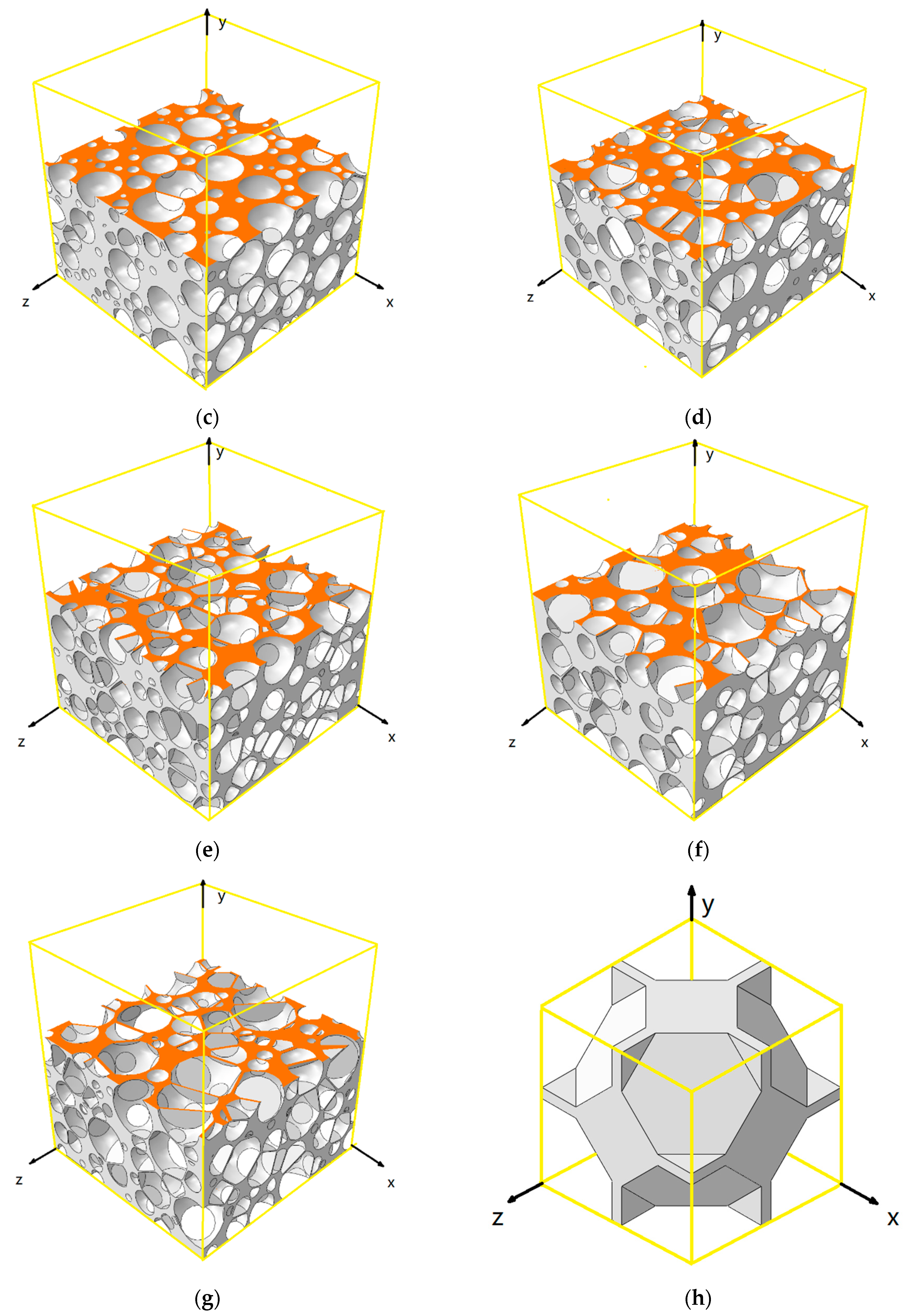
The representative volume element (RVE) approach is often used in the literature. By using this method, classical homogenization over the micro-scale domain can be used to analyze the mechanical property at the macroscopic scale. RVE is a micro-scale model of the material used to determine the corresponding homogenized/effective properties at the macroscopic scale. For foam material, the cubic RVE model contains cell wall material and pores. A random modeling procedure that builds closed-cell foam models with various cell structures was proposed by Hu et al. [32,33,34]. The mechanical properties of foam material are influenced by bulk material and relative density. However, the research on inner structure is not confined to the Voronoi model. The Voronoi model is put to wide use in simulation, and the disturbance factor can describe the randomness of the inner structure, but there is no method to measure the disturbance factor for the experiment in practice. Different from the Voronoi model, Hu uses characteristic diameter D c h and characteristic shape anisotropy α c h defined based on the two-dimensional geometric parameters to reflect the inhomogeneity in cell size distribution and irregularity in cell shape for the 3D foam materials. When the area fraction of the pores whose diameters are larger than d in the total area of pores is 0.2, this diameter is the characteristic diameter D c h . As the characteristic diameter D c h increases, the bigger pores in random model are more vulnerable generated. Taking the facts into account, the range of characteristic diameter D c h is set as (3.11–3.79), as shown in Table 1. For characteristic shape anisotropy α c h , α c h = 0 represents that all pores in the random model are nearly spherical pores. As characteristic shape anisotropy α c h increases, the shape of the big pores is more promiscuous. Figure 1 shows the random models with different characteristic diameter D c h and characteristic shape anisotropy α c h . And the characteristic diameter D c h and characteristic shape anisotropy α c h can be measured in experiments. The characteristic diameter D c h and characteristic shape anisotropy α c h are calculated cross section of the random model cubic. There are six cross sections, which are perpendicular to the x, y, and z axis. The Model 1 and Model 2 with α c h = 0 only have sphere cells as shown in Figure 1a,b. It shows that there are more large pores with the increasing of the characteristic diameter D c h . The Models 3–7 with α c h > 0 have polyhedron cells as shown in Figure 1c–g. It shows that the large pores are more irregular as the characteristic shape anisotropy α c h increases. And the characteristic diameter D c h and characteristic shape anisotropy α c h can be measured in experiments. The characteristic diameter D c h and characteristic shape anisotropy α c h are calculated cross section of the random model cubic. There are six the cross sections, which are perpendicular to the x, y, and z axis. Meanwhile, the researchers in [35,36] proposed that a rectangular cube with at least five cellular pores on each edge and more than 125 cellular pores overall can be utilized to investigate the mechanical properties. And the simulation results corroborate the experimental findings well. Therefore, the RVE thus has dimensions of 14 mm in height, breadth, and depth, which are sufficient to meet RVE’s requirements for material size.
Compared with the random model above, we also use the Kelvin model of RVE, which regularly has a body centered cubic (BCC) lattice of cells to explore the mechanical property. So we can use a few cells as RVE because of the periodic and symmetric properties of the Kelvin model. The RVE is a cuboid with a height, width, and depth of 2 2 mm, as shown in Figure 1h.

2.2. Mechanical Properties of Bulk Materials

We choose the aluminum alloy as the cell wall material because many researchers [2,3,4,5,6,8,9,10,11,12,13,14,16] investigated the mechanical properties of aluminum alloy via experiments in past years. So, in this work, aluminum alloy is selected as the bulk material of the foam model. As shown in Table 2, the bulk material is nearly the same as the Al alloy in Su et al. [37]. And according to Su et al. [37], the constitutive relation of the Al alloy in the plastic region can be written as Formula (1),
  σ = σ 0 + E p 1 exp 8.3 ε p
where σ and ε p are the engineering stress and plastic strain at the plastic stage; σ 0   and E p are the yield strength and plastic modulus.

2.3. Basic Loading Conditions

The coordinate system of the random and Kelvin model RVE is shown in Figure 1a, 1b, and 1c, respectively. Symmetrical boundary conditions are applied on the surfaces of x = 0   mm ,   y = 0   mm , and z = 0   mm , respectively. For random models, surface traction load P x is applied on the cell wall in the surface of x = 14   mm ; surface traction load P y is applied on the cell wall in the surface of y = 14   mm; surface traction load P z is applied on the cell wall in the surface of z = 14   m m. And surface traction load conditions ( P x , P y and P z ) are applied on the cell wall in the surfaces of x = 2 2 mm ,   y = 2 2 mm , and z = 2 2   mm for the Kelvin RVE, respectively. The traction stress load guarantees that the ratio of cross-section stress along the x, y, and z axis stays constant during the loading process. The coupling conditions are applied between all the nodes on the load surfaces along the x, y, and z axis and corresponding reference points, respectively, to enforce that all the nodes on the surfaces have the same displacement. So that the surfaces are kept to be plane.
The nonlinear geometry (NLGEOM) algorithm is applied in the simulations to consider the geometric nonlinearity of the model during the loading process.

2.4. The Macro Normal Stresses and Strain

Based on the RVE approach, we need to obtain the average stresses and strains on the cross section of RVE in the x, y, and z directions. The cross-section stresses on the surfaces of the RVE models (representing the average stresses in the RVE) are given in Formula (2), considering the RVE model as a continuous material,
σ x x = F x S x ,   σ y y = F y S y ,   σ z z = F z S z
where F x , F y and F z are the sum of the reaction force obtained on the three cross sections x = 0   mm , y = 0   mm , z = 0   mm , which are perpendicular to coordinates x, y, and z, respectively, S x , S y , and S z are the area of the corresponding cross-sections of the cubic RVE, σ x x ,   σ y y , and σ z z   are the corresponding (macro) stresses of the RVE.
The engineering strains in the foam (representing the average strain in the RVE) are obtained with Formula (3),
  ε x x = U x L x ,   ε y y = U y L y ,     ε z z = U z L z
where L x , L y , and L z are the height, width, and depth of the RVE, U x , U y and U z are the relative displacements of the cross sections between x = 0 and x = L x , between y = 0 and y = L y , between z = 0 and z = L z , respectively; ε x x ,   ε y y   and ε z z are the corresponding (macro) strains of the cubic RVE.

2.5. Mesh Convergence Analysis

The quadratic element has higher calculation accuracy than the linear element. And modified mesh is more suitable for large deformation. Then, the modified quadratic tetrahedron element (C3D10 M) is used to mesh the closed-cell foam model in order to obtain more accurate simulation results under certain conditions. Table 3 shows the number of elements in a random model with different element sizes.
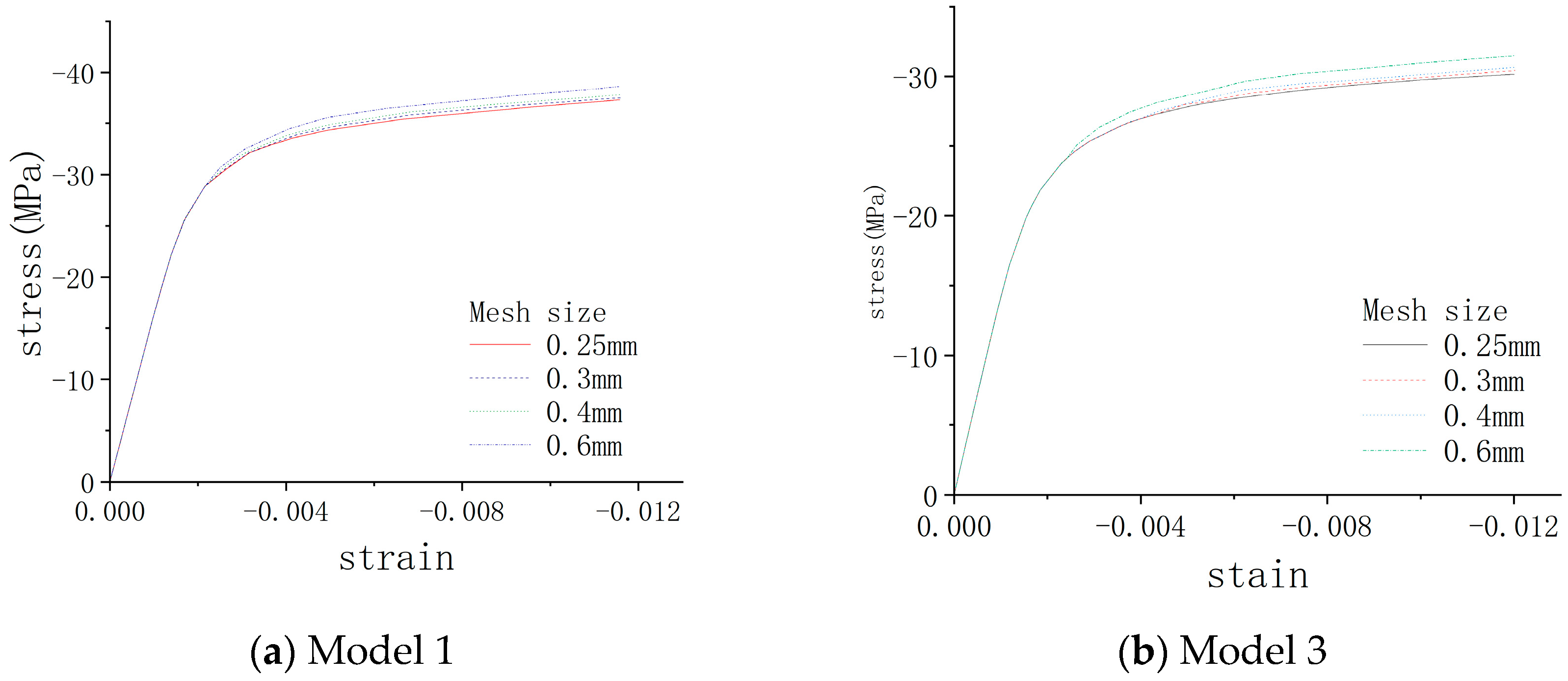
Table 3 shows the number of elements increases sharply while reducing the element size. In order to select the element size, Figure 2 give the stress-strain response curve of three random models under uniaxial compression. It shows that the curves of the random model with element size 0.25 mm and 0.3 mm are nearly consistent. So we use 0.3 mm as the element size for different random models in our study.
Because of the regular cell wall in the Kelvin model, we can use the hexahedral element to mesh. So C3D8I is used for the simulation of the regular Kelvin model. Since the Kelvin model in Figure 1h is simple, the number of elements is smaller, so we do not discuss mesh convergence analysis.

2.6. Multiaxial Loading Conditions

The multiaxial loading states in this work are axisymmetric compression and tension as they are commonly seen in experiments. Three normal loads (including tension and compression) are applied proportionally to the RVE. Since the RVE models are cubes and the model used is homogenous at the macro-scale, the stresses σ x x ,   σ y y , and σ z z herein are normal stresses along the x, y, and z axis of the RVE. Where the shear stresses ( τ x y , τ y z and τ x z ) are equal to zero, so that the normal stresses ( σ x x ,   σ y y and σ z z ) are the principal stress. Because of the similar structures in the x, y, and z directions, we can choose any of the x, y, and z directions as the principal loading direction in the simulation, and the results would be similar. In the simulation, the loading condition is chosen to let the normal stress σ x x σ y y   σ z z . So the x, y, and z direction of RVE is chosen as the direction of principal stress σ 1 , σ 2 and σ 3 in all of the following numerical simulations, respectively.
In the principal-stress space,   σ 1 σ 2 σ 3 holds. The permissible region should be the intersection between the area of σ 1 σ 2 and the area of σ 2 σ 3 . The limits for this permissible region are the σ 1 = σ 2 plane and the σ 2 = σ 3 plane, respectively. The intersection of the two planes of σ 1 = σ 2 and σ 2 = σ 3 is the hydrostatic stress state. The Lode angle 𝜃 is the included angle between the σ 1 = σ 2   plane and the plane that passes through the hydrostatic axis. Wu et al. [29] and Serban [38] investigated the influence of the triaxial state of stress on the failure and yield of foam. The range of 𝜃 is 0° ≤ 𝜃 ≤ 60°. Formulas (4) and (5) are the expressions of triaxial stress ratio k and Lode angle 𝜃, respectively,
  k = σ e σ m = 1 2 σ 1 σ 2 2 + σ 2 σ 3 2 + σ 1 σ 3 2 σ 1 + σ 2 + σ 3 / 3
cos 3 θ = 27 σ 1 σ m σ 2 σ m σ 3 σ m 2 σ e 3
where σ e is Mises equivalent stress, σ m is mean stress. However, due to the lack of tension experimental data, only the yield behavior for σ m 0 in the σ e σ m space is investigated. In the study of Wu et al. [29], the position of the yield point in the σ e σ m space is determined by the value of k as well as cos 3 θ . To ensure that the yield points are evenly distributed in the σ e σ m space, the triaxial stress ratio k is set as , 3 , 1.5 , 1 , 0.6 , 0.3 ,   0 . The value of cos 3 θ is set as −1, 0, and 1. So the yield surface contains sufficient data, including uniaxial compression, biaxial compression, tri-axial compression, and combined compression-tension load. Table 4 presents the principal stress ratio schemes used in the numerical simulations.

3. Results and Discussion

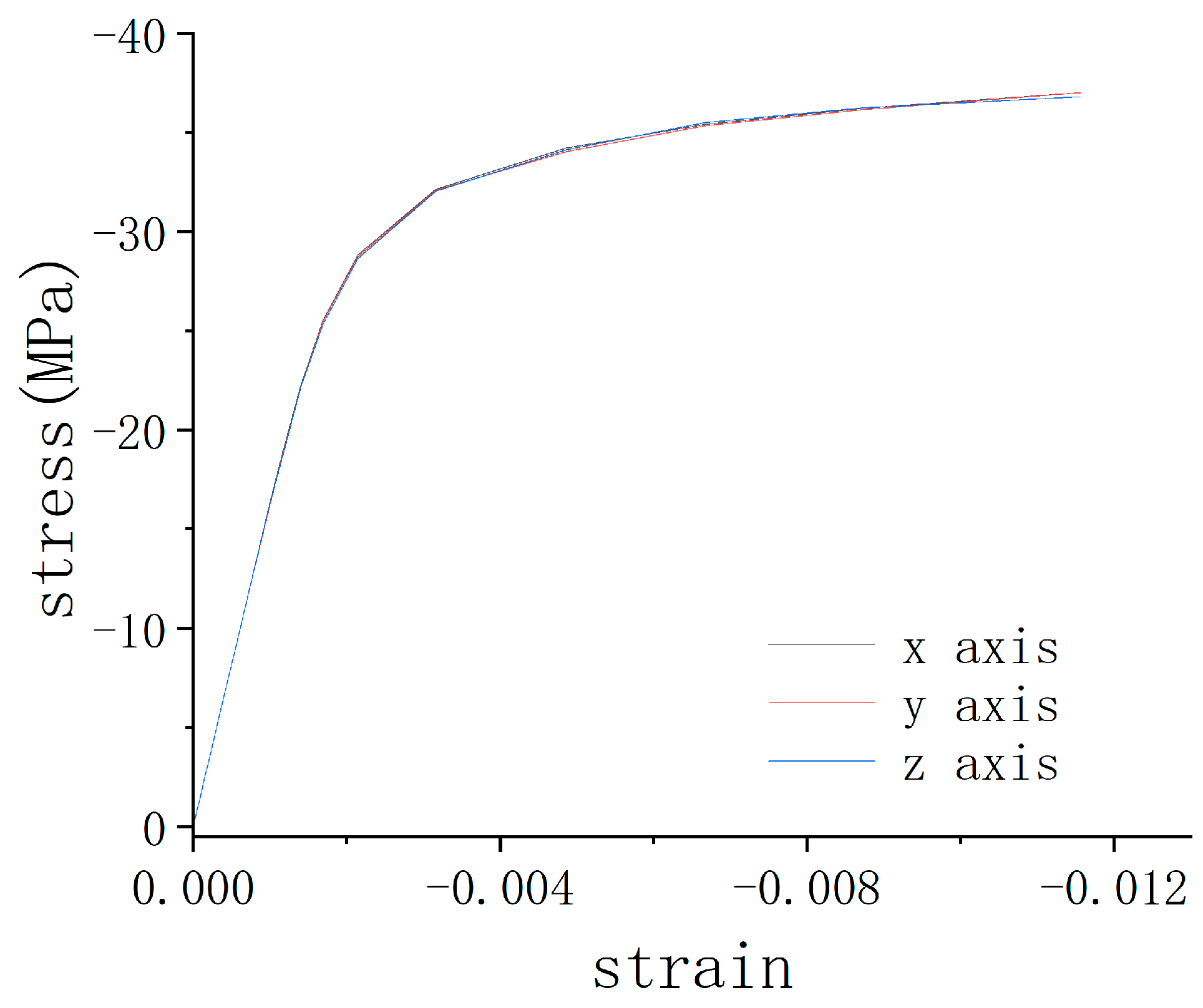
Figure 3 shows the stress-strain response curve of the foam material under the uniaxial state. Although foam is non-continuum, it also changes from linear to nonlinear. When the loading is small, the stress-strain response is linear. With the increasing of loading, the micro part of the foam begins to yield making the increase in amplitude of stress decrease with the increasing of strain. And when more of the foam yields, the stress-strain response curve of the foam material becomes nonlinear. In order to verify, we give the stress-strain response curves along the x, y, and z axis of the RVE cubic. Figure 3 shows that the stress-strain response curves along the x axis is almost coincided with that along the y and z axis. It is generally known in [15,16,19,29,30,31] that the yield points under the multiaxial loadings are mainly determined by two methods. One is obtained at 0.2% characteristic strain offset on the characteristic stress-strain curves (Figure 4 and Figure 5). The other is given in terms of the plastic dissipation energy.
Because there is a large number of yield points of different RVE models, we exclusively utilize Kelvin RVE with relative densities of 0.20 and 0.43, and Models 1 and 6 (in Table 1) with relative densities of 0.4 and 0.3, respectively, to investigate the yield surface of closed-cell foam. This can make the data comparison with the experiments more clear. So we use these RVEs to explore the yield definition under multiaxial loadings in the following section.

3.1. Yield Points Defined by 0.2% offset of the Characteristic Plastic Strain

The characteristic stress σ ¯ and strain ε ¯ were given in Formulas (6)–(12),
σ ¯ = σ e 2 + β 2 σ m 2
ε ¯ = ε e 2 + ε m 2 / β 2
where σ e and σ m are the Mises effective stress and mean stress, respectively,
σ e = 1 2 [ σ 1 σ 2 2 + σ 2 σ 3 2 + σ 3 σ 1 2 ]
σ m = σ 1 + σ 2 + σ 3 3
where ε e and ε m are corresponding Mises effective strain and mean strain, respectively,
ε e = 2 9 ε 1 ε 2 2 + ε 2 ε 3 2 + ε 3 ε 1 2
ε m = ε 1 + ε 2 + ε 3
where β 2 is a material parameter associated with the Poisson ratio ν , defined as
β 2 = 9 1 2 ν 2 1 + ν
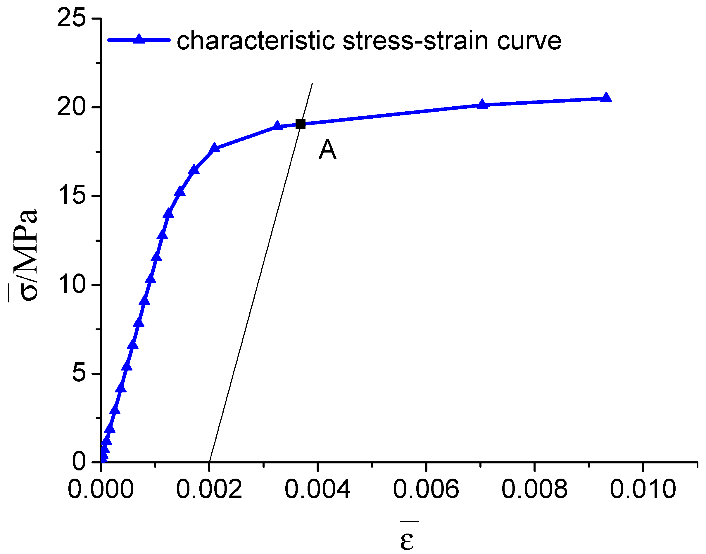
With the characteristic stress σ ¯ and strain ε ¯ given above, the characteristic stress-strain curves of different models under uniaxial compression and multiaxial load state can be established. Figure 4 shows the uniaxial principal compression stress-strain curve and corresponding characteristic stress-strain curve for the Kelvin model with a relative density of 0.2. Figure 5 shows the corresponding characteristic stress-strain curve of the multiaxial load process. The yield points defined by 0.2% offset of characteristic plastic strain are shown as point A in Figure 4 and Figure 5. In Figure 4, the yield point defined by 0.2% offset of the principal plastic strain is also shown at point B. It is shown that there is little difference between the yield points defined by the characteristic plastic strain method and the principal plastic strain method. The difference is due to the compressibility of the foam material. The yield points defined by the 0.2% characteristic strain offset method for different foam models under multiaxial load states can be obtained.
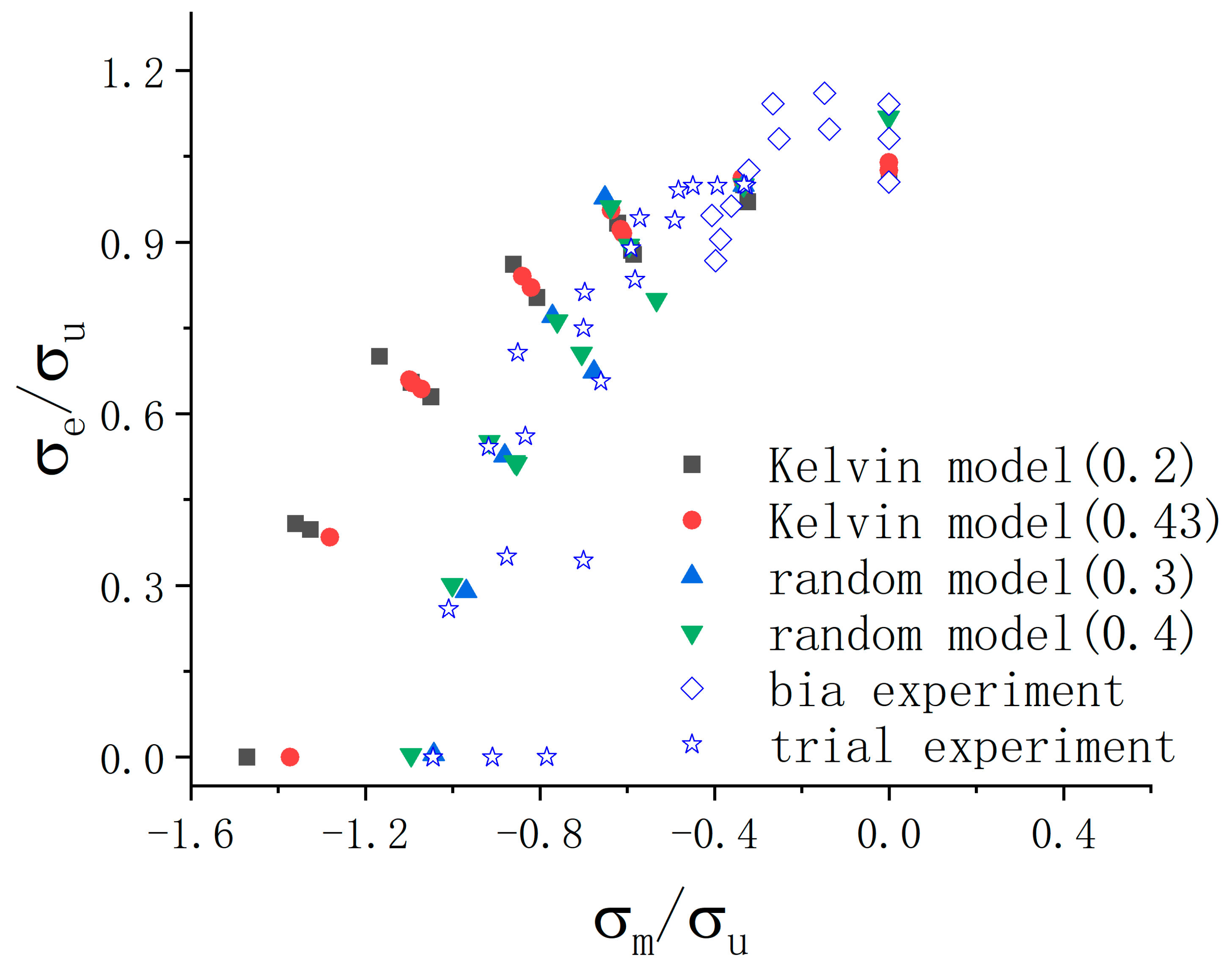
The cell wall materials used in the numerical simulation and experiments are not identical. So the comparison of different aluminum alloys as cell wall materials can have little significance. To solve this problem, we give a comparison of dimensionless yield surfaces. To give a normalized yield surface, the uniaxial compression yield stress σ u is used to nondimensionalize the yield points ( σ m / σ u , σ e / σ u ) in the σ m / σ u σ e / σ u space. The uniaxial compression yield stress σ u is obtained with the method shown as point B in Figure 4. The normalized yield points ( σ m / σ u , σ e / σ u ) for each model are plotted in the following σ m / σ u σ e / σ u space. Among them, the yield surface defined by 0.2% offset of the characteristic plastic strain is shown in Figure 6. It shows that, for the isotropic Kelvin RVE, the yield surface for the aluminum alloy foam with a relative density of 0.2 is a little larger than the yield surface for the foam with a relative density of 0.43, especially for the loading states close to the σ m   axis. For the random RVE model, the difference in the yield surface with different relative densities is small. It can also find that there is a larger scatter on the yield surface for the load ratio with the value of k in the range of −0.3 and −1.5 for both models. It means that the yield surface defined by this method depends not only on σ m and σ e , but also on other stress state characters, such as the value of cos 3 θ . The biaxial experiment data given in [4] and triaxial experiment data given in [9] are also shown in Figure 6. It is shown that the yield surface obtained with the method is at the outside of the experiment data points.

3.2. Yield Points Defined by the Critical Plastic Dissipation Energy

For the multiaxial loads, the initial yield of the closed foam could also be judged by the critical plastic dissipation energy [29,30]. The critical plastic dissipation energy value is given as the plastic dissipation energy per unit volume at point B in Figure 4, which is defined by 0.2% offset of plastic strain on the uniaxial principal compression stress-strain curve. The yield points under multiaxial load states are defined by the condition that the plastic dissipation energy per unit volume reaches the critical plastic dissipation energy value per unit volume. For the Kelvin model with 0.2 relative density, the plastic dissipation energy per unit volume is 22.8 × 10⁻³ mJ/mm3; with 0.43 relative density, the plastic dissipation energy per unit volume is 60.6 × 10⁻³ mJ/mm3; for the random model 6 (in Table 1) with 0.3 relative density, the plastic dissipation energy per unit volume is 20.1 × 10⁻³ mJ/mm3; for model 1 (in Table 1) with 0.4 relative density, the plastic dissipation energy per unit volume is 57.3 × 10⁻³ mJ/mm3. Table 5 shows the plastic dissipation energy per unit volume for different models with different related densities and inner structure. It is presented that the plastic dissipation energy per unit volume at yield point is not subject solely to the influence of the related density of the foam material. However, the inner structure also affects the plastic dissipation energy per unit volume. And the plastic dissipation energy per unit volume at the yield point of the regular Kelvin model is bigger that that of the random model.
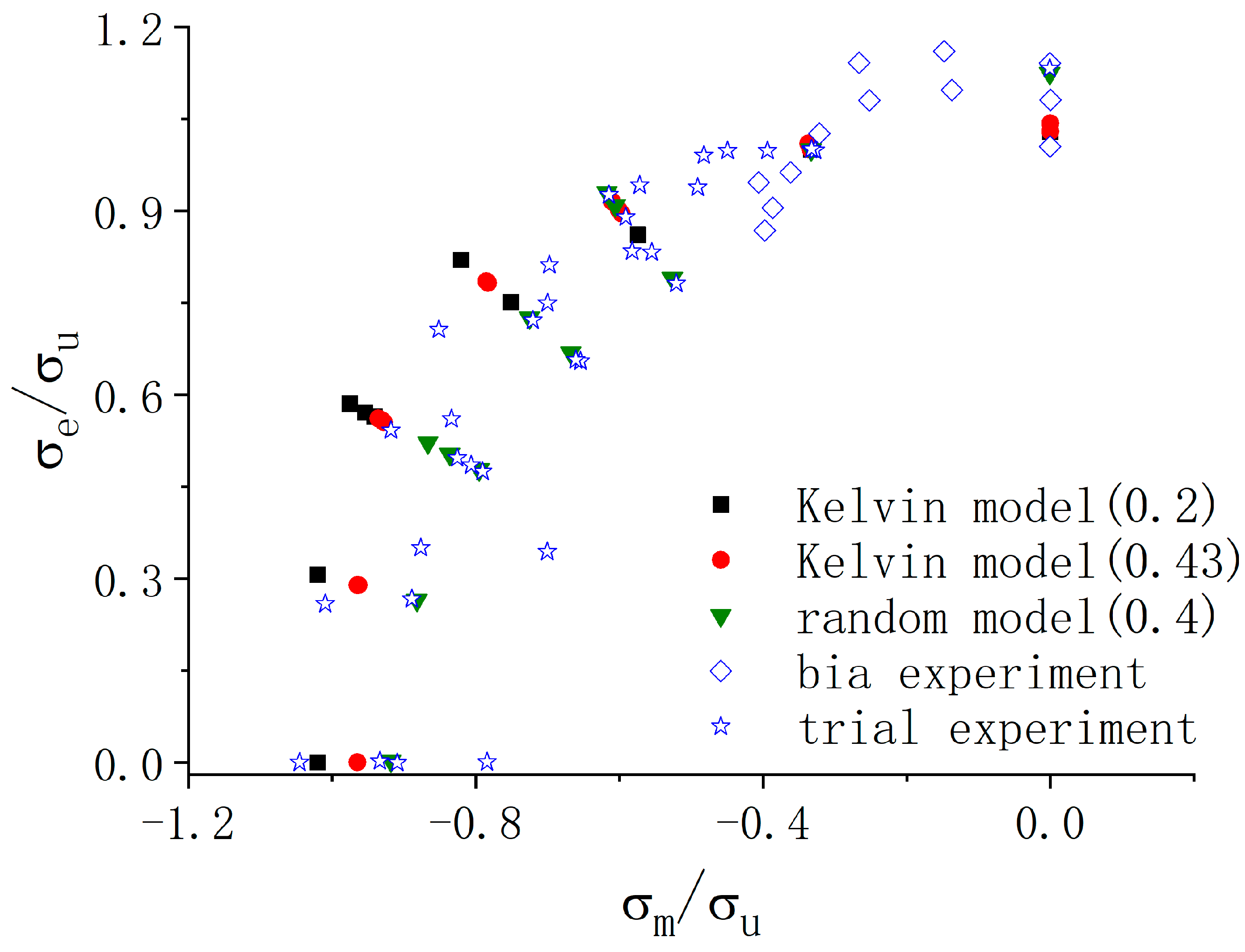
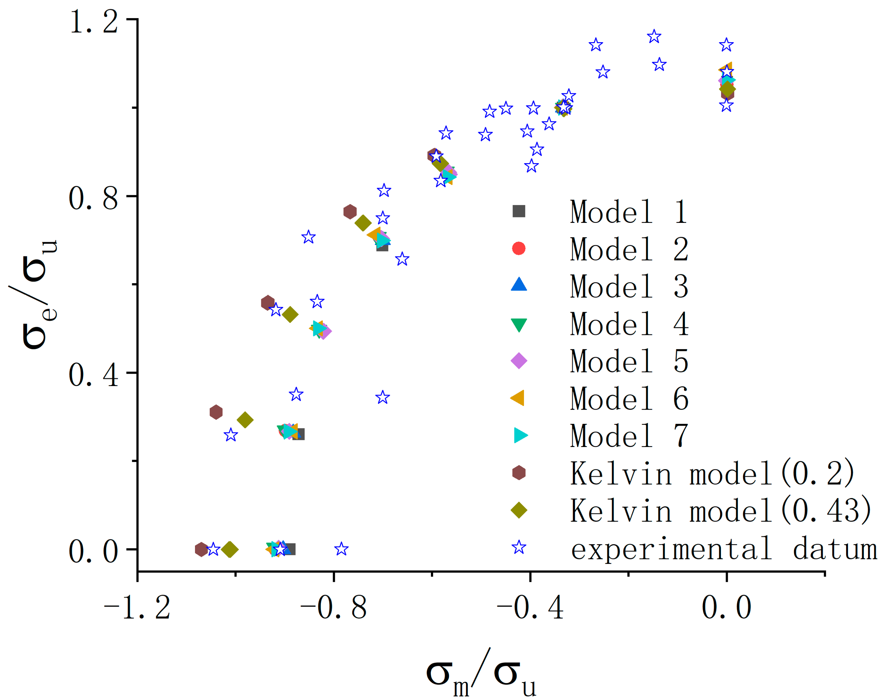
Figure 7 gives the normalized yield points ( σ m / σ u , σ e / σ u ) given by the critical plastic dissipation energy in the σ m σ e space using the Kelvin model with relative densities of 0.2 and 0.43, and models 6 and 1, in Table 1, with relative densities of 0.3 and 0.4, respectively. Additionally, like Figure 5, Figure 6 also implies that parameter cos 3 θ affects the distribution of yield points defined by this method because of the scatter of yield points for the given value of parameter k in the σ m / σ u σ e / σ u space. For the comparison of the yield surfaces obtained by the numerical simulation and available literature biaxial experimental data [4] and triaxial experimental data [9], the result is similar to that in Figure 6. It is shown that the yield surfaces obtained by the numerical simulation are in good accordance with experimental data close to the   σ e / σ u axis, but there is a larger difference with the stress state close to the σ m / σ u axis.
Overall, contrasting the data, the results demonstrate that the yield surfaces defined by these two yield definition methods above can not only be described by σ m and σ e . The parameter k would also skew the distribution of yield points in the σ m / σ u σ e / σ u space. Meanwhile, there is a large difference between the numerical simulation datum and experimental datum near σ m / σ u axis. Therefore, more suitable definitions of yield points should be explored.

3.3. Yield Points Defined by the Critical Plastic Dissipation Energy at the Microscopic Scale

Since the yield points determined by the yield definition methods given above are not consistent with the experimental datum, other kinds of yield definition methods should be explored. It is found that the ability of volumetric deformation of closed-cell foam materials must be considered because the great difference between simulation results and experimental results occurred mainly near the σ m / σ u axis. Therefore, the yield definition based on plastic dissipation energy could be improved by including the volumetric deformation energy.
At the microscopic scale, the internal deformation of the wall material is commonly divided into two parts: volumetric deformation and distortional deformation. Theoretically, the total energy, plastic dissipation energy, and volumetric deformation energy of the RVE at any time t can be calculated with the following equations,
  E t = 0 t ( V σ x x ε ˙ x x + σ y y ε ˙ y y + σ z z ε ˙ z z + 2 σ x y ε ˙ x y + σ y z ε ˙ y z + σ x z ε ˙ x z d V ) d t
  E p = 0 t ( V σ x x ε ˙ x x p + σ y y ε ˙ y y p + σ z z ε ˙ z z p + 2 σ x y ε ˙ x y p + σ y z ε ˙ y z p + σ x z ε ˙ x z p d V ) d t
  E V = 0 t ( V σ x x + σ y y + σ z z / 3 ε ˙ x x + ε ˙ y y + ε ˙ z z d V ) d t
where E t , E p , and E V indicates total energy, plastic dissipation energy, and volumetric deformation energy, respectively, σ x x , σ y y , σ z z , σ x y , σ y z , σ x z   are components of the stress tensor in the cell wall material, ε ˙ x x , ε ˙ y y , ε ˙ z z , ε ˙ x y , ε ˙ y z , ε ˙ x z are components of the strain rate tensor, ε ˙ x x p , ε ˙ y y p , ε ˙ z z p , ε ˙ x y p , ε ˙ y z p , ε ˙ x z p are plastic strain rates, and V is the total volume of the cell wall material. E t ,   E p , and E V (Formulas (13)–(15)) can be numerically evaluated during the finite element analysis.
With the energy obtained with Formulas (13)–(15), a critical parameter E c r i at yield points can be assigned to E p + M E V per unit RVE volume at point B in Figure 4. Similarly, for the case of the multiaxial stress state, the yield point is also thought to be reached when E p + M E V per unit RVE volume equals the critical parameter, where M is an empirical weight coefficient
By comparison with biaxial and triaxial experiments given in [4,11] respectively, it can be found that the value of M = 4 is a suitable weight coefficient of the volumetric deformation energy in the yield point definition. For the Kelvin model RVE with a relative density of 0.2, the critical parameter is 28.9 × 10⁻³ mJ/mm3; with a relative density of 0.43, the critical parameter is 79.8 × 10⁻³ mJ/mm3; for the random model 6 (Table 1) RVE with a relative density of 0.4, the critical parameter is 76.3 × 10⁻³ mJ/mm3.
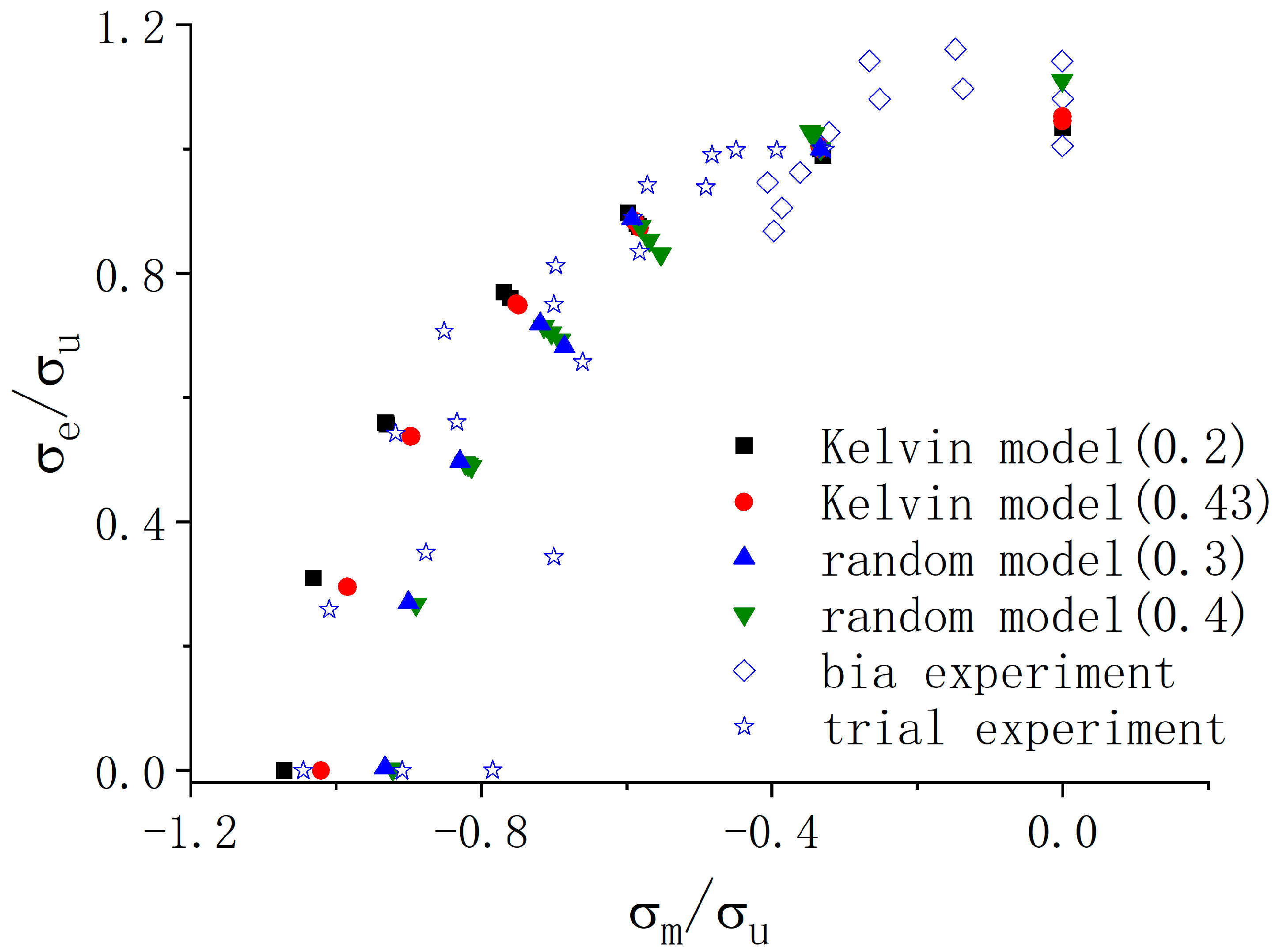
Figure 8 shows that the yield surface for the Kelvin model with a relative density of 0.2 is on the outside of that for the Kelvin model with a relative density of 0.43. The yield surface of the random model with a relative density of 0.4 is on the inside of the yield surface for the Kelvin model. It also shows that the yield surface defined by this method depends not only on σ m and σ e , but also on the value of cos 3 θ . It is shown in Figure 8 that the yield surfaces based on the critical parameter given above fit better with the experimental datum. Although the yield definition method with the critical parameter can describe the yield surface of foam material under multiaxial stress states well, it is not convenient using this method to capture the yield state with macro-scale stresses of foam materials.

3.4. Yield Points Defined by the Critical Characteristic Energy E c h

To reduce the effect of cos 3 θ , we try to use the elastic energy stored per unit RVE volume as a critical characteristic energy E c h to judge the yield state of the foam material. Based on the micro-scale relationship between the three types of energy from Formulas (13) and (14), the elastic energy stored is given by Formula (16).
  E e = E t E p
The critical character energy E c h is defined as the E e at the yield point B in Figure 2 divided by the volume of the RVE used in the simulation. It is given as Formula (14),
  E c h = E e / V R V E
where V R V E is the volume of the RVE used in the simulation.
For the Kelvin model with 0.2 relative density, E c h is 20.7 × 10⁻³ mJ/mm3; with 0.43 relative density, E c h is 47.8 × 10⁻³ mJ/mm3; for the random model 6 (in Table 1) with 0.3 relative density, E c h is 19.4 × 10⁻³ mJ/mm3; with 0.4 relative density, E c h of the random model 1 (in Table 1) is 38.3 × 10⁻³ mJ/mm3. The yield point under multiaxial stress states is obtained when their E e / V R V E is equal to E c h .
Figure 9 gives the yield surfaces defined by E c h based on the micro-scale for the Kelvin model with 0.2 and 0.43 relative density and the random model with 0.3 and 0.4 relative density. Compared with the yield surfaces given above in Figure 6, Figure 7 and Figure 8, the scattering of yield points for the same value of parameter k is significantly reduced. The effect of the value of cos 3 θ is much smaller on the yield surface defined by E c h than on the yield surfaces given by the previous three yield definition methods. Meanwhile, relative density does not affect the yield surface for random models. It is also shown that the yield surfaces using the Kelvin model and random model defined with E c h are consistent with the experimental data, which covers the scatter of the experimental data. And the biaxial experimental data is given in [4], the triaxial experimental data is given in [9]. So this critical characteristic energy E c h based on a micro-scale can be used to define the yielding of closed foam. This critical characteristic energy E c h should be derived by finite simulation tests. The method of determining yield points is not sufficient for the experimental tests.

3.5. Yield Points Defined by the Critical Characteristic Energy W

To derive a more convenient method to define the yield state macroscopically, we use the stress tensor of RVE in Formula (2) to define the yield of closed foam material. It is reported that the elastic energy stored per unit RVE volume E e / V R V E can be approximately represented with W given by Formula (18) macroscopically in [39],
W = 1 2 E ¯ σ e 2 + β 2 σ m 2
where β is the material constant defined by Formula (19), and E ¯ is defined by,
E ¯ = 3 E 2 1 + ν
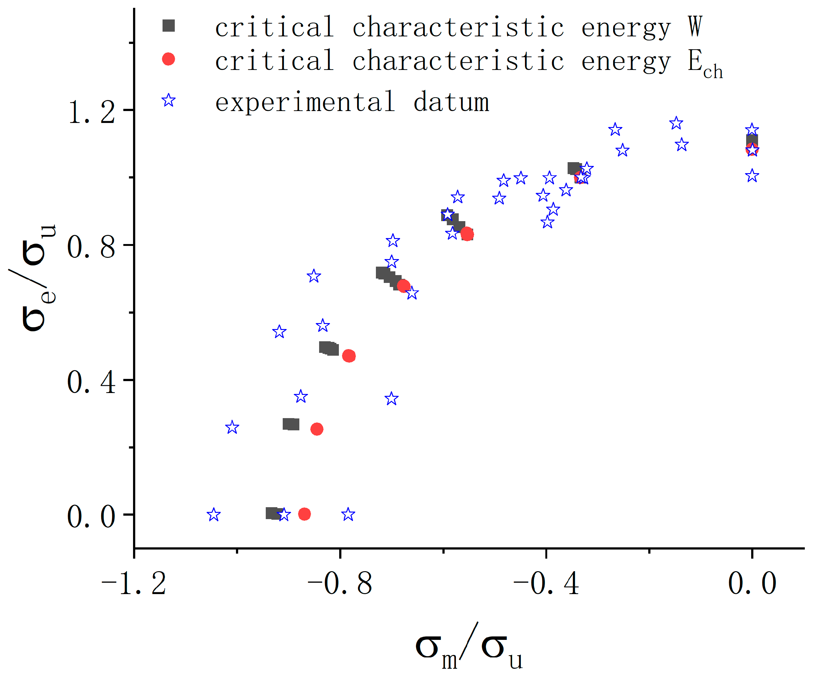
Table 6 gives the E c h and W for the random model 1 with 0.4 relative density under different multiaxial stress states. It is shown that the W is not equal to E c h and varies with the stress state. So we give yield surfaces defined by the critical characteristic energy E c h and W in Figure 10, respectively. It shows that the yield surface defined by the critical characteristic energy W is bigger than that defined by the critical characteristic energy E c h , especially near σ m / σ u axis. So we cannot use the value of W at the yield point B in Figure 4 to define the yield of the RVE. To propose a more proper engineering yield definition method, we can reformulate Formula (18).
To do this, we propose Formula (20), which is modified for Formula (18), to represent the elastic energy per unit volume of RVE based on macro-scale stresses as follows,
W = 1 2 E ¯ σ e 2 + 1 ρ A + β 2 σ m 2
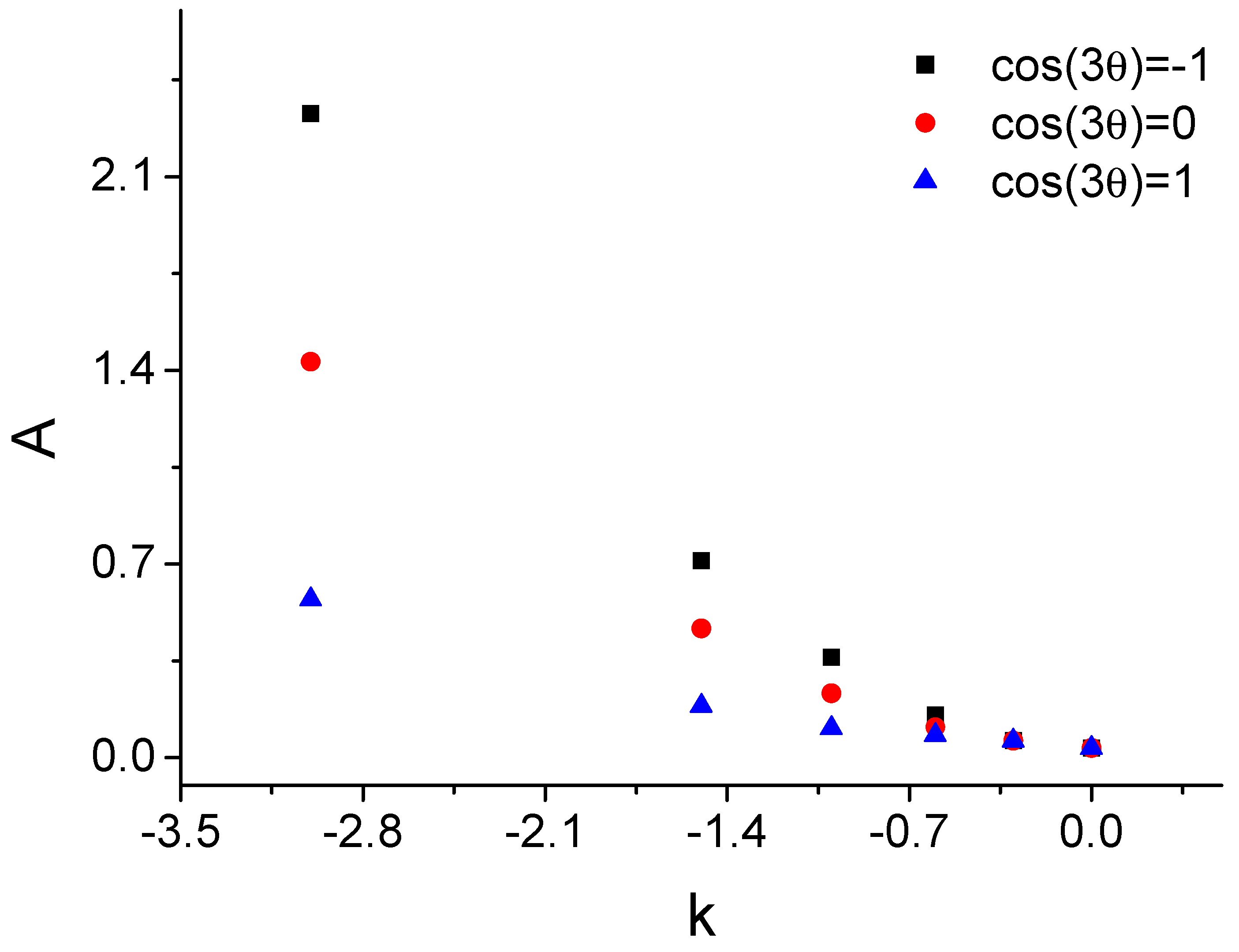
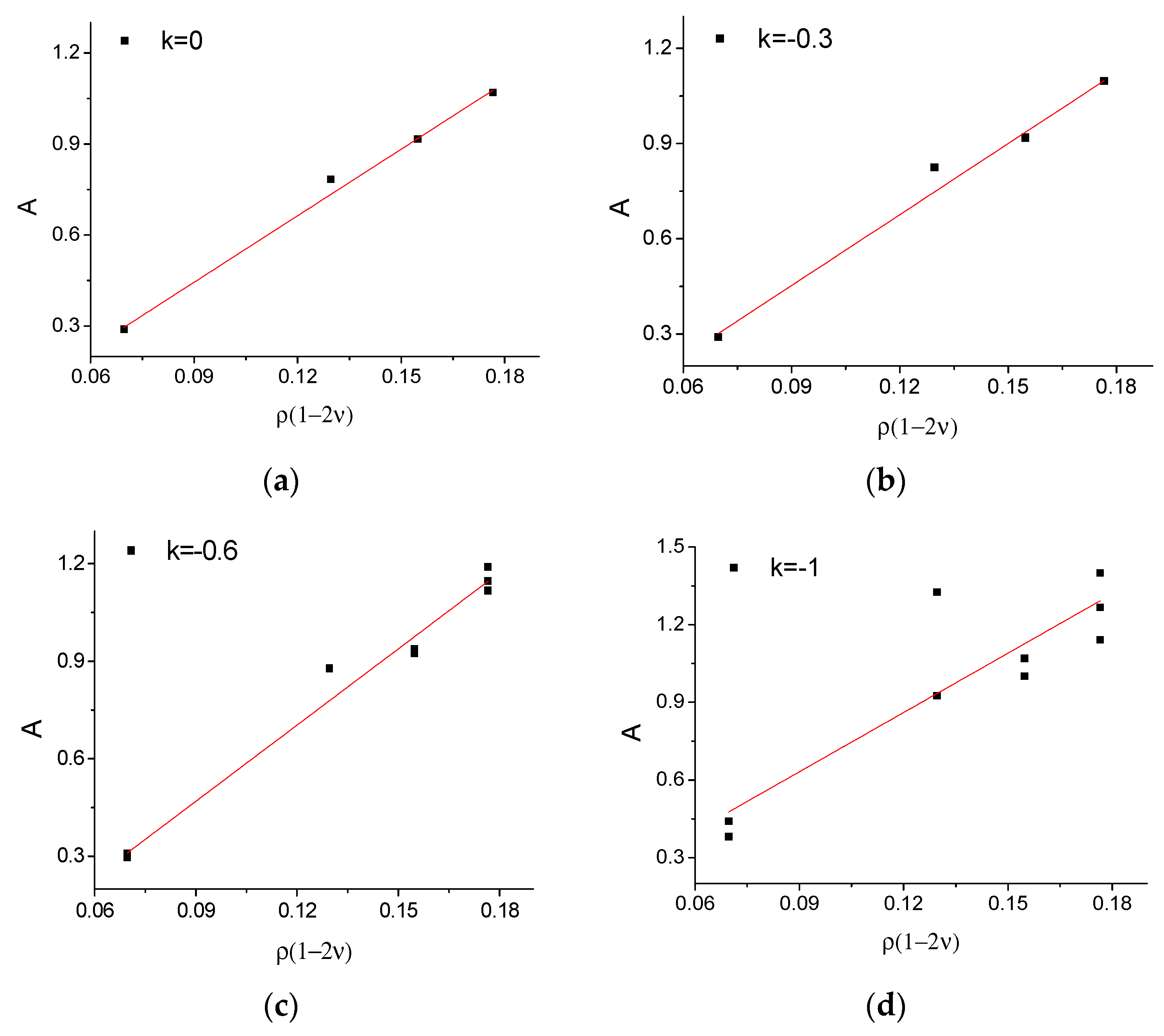
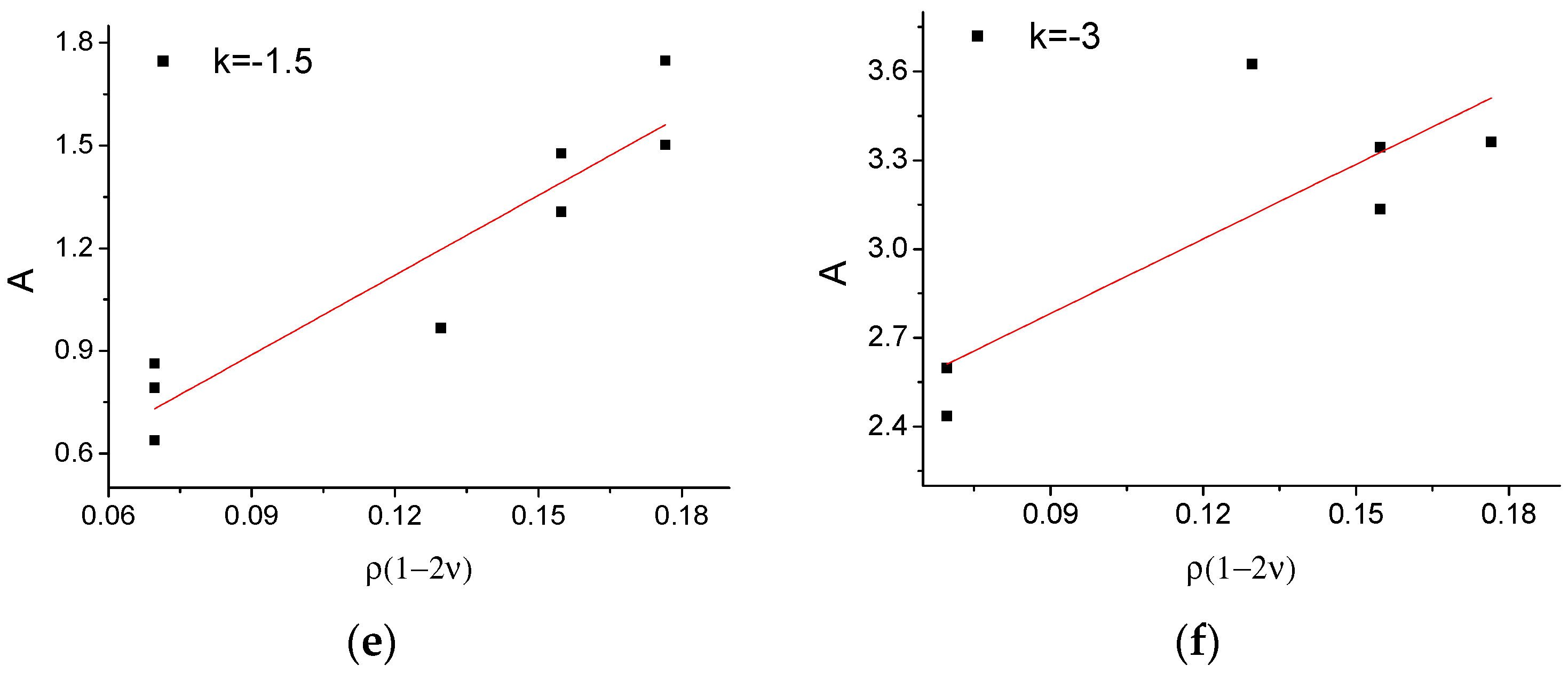
Let W = E c h , and we can get the value of coefficient A for different stress states. Figure 11 shows that the coefficient A changes as a function of the stress-proportional parameter k and cos 3 θ . As shown in Figure 9, the effect of cos 3 θ on the yield surface is small, so only the effect of the parameter k is considered in the following discussion. Figure 12 shows the relationship between parameter A and ρ 1 2 ν for different values of k. It is shown that the coefficient A scales linearly with the ρ 1 2 ν at several fixed values of parameter k. Therefore, parameter A can be written as Formula (21),
  A = 0.2 + 0.2 k + 0.3 k 2 + 7.4 0.3 k ρ 1 2 ν
With Formulas (20) and (21), the value of W at yield point B in Figure 9 can be obtained and is defined as the critical value W c h . The values of W c h   are 20.7 × 10⁻³ mJ/mm3, 47.8 × 10⁻³ mJ/mm3 for the Kelvin model with relative densities of 0.20 and 0.43, and 19.4 × 10⁻³ mJ/mm3, 38.3 × 10⁻³ mJ/mm3 for the random model with relative densities of 0.3 and 0.4. The yield point under multiaxial load states is obtained when W is equal to W c h .
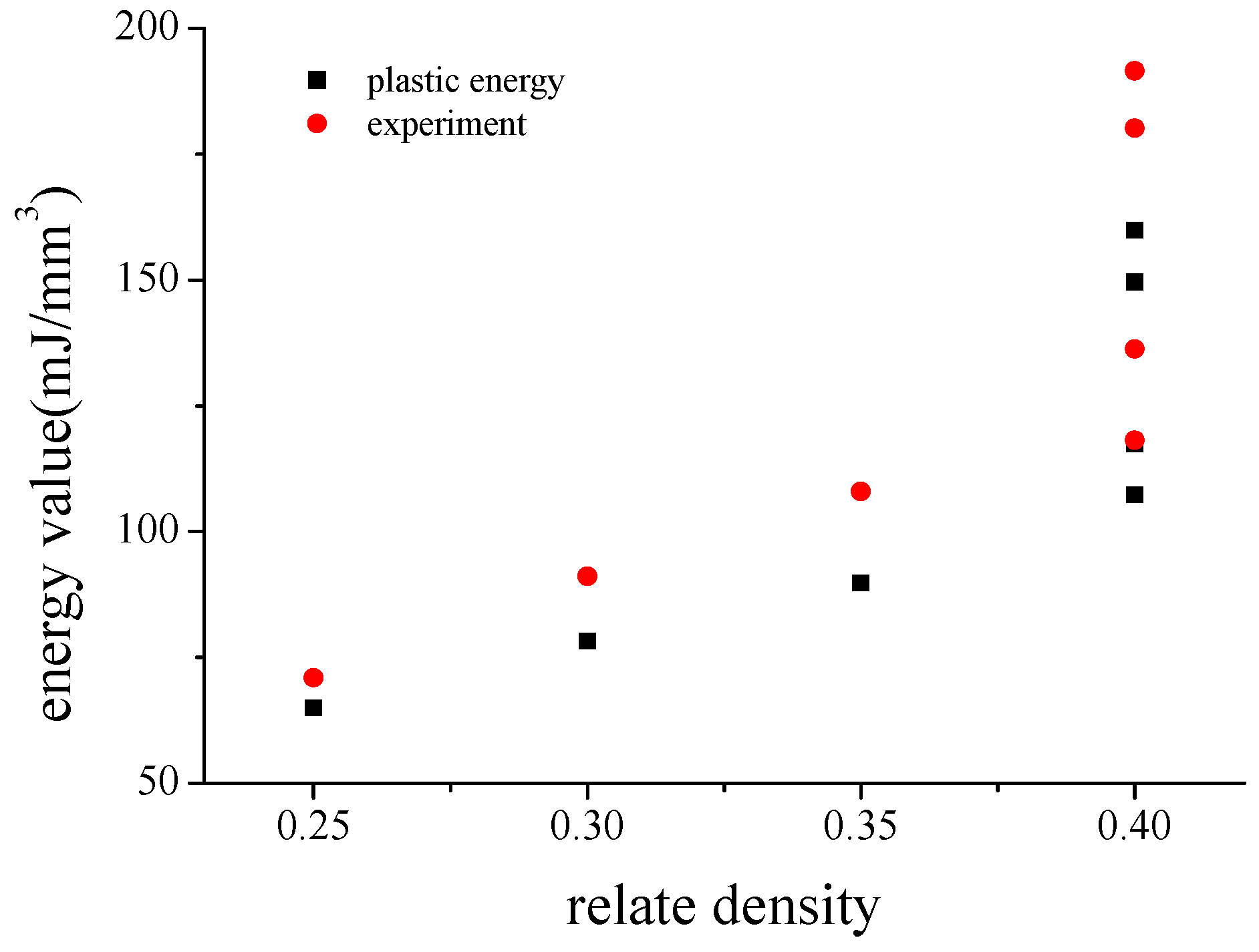
The following Figure 13 gives the energy values obtained with the plasticity models in the experiment. It shows that the the energy value obtained by the experiment is bigger than that obtained with the plasticity models. And with the increasing of relative density, the energy values increase. However, the energy values are also dependent on characteristic diameter D c h and characteristic shape anisotropy α c h . Because of the characteristic diameter D c h with a small difference, we only discuss the effect of the characteristic shape anisotropy α c h on the difference energy values. Figure 14 gives the effect of the characteristic shape anisotropy α c h . And this effect can be fitted by the quadratic formula. It shows that the difference between the energy values obtained with the plasticity models and the experiment decreases as characteristic shape anisotropy α c h increases.
To test, we use all models in Table 1 to determine whether these equations apply to models with different inner structures. Figure 15 gives yield points defined by the critical characteristic energy W based on macro-scale stresses.
Figure 15 compares the yield surfaces defined by the yield method in Formulas (20) and (21) for the Kelvin and random RVE models with the experimental datum. Different from the yield definition methods in the literature, the yield surface defined by this method depends on σ e and σ m only. It also shows that the surfaces determined by this yield definition method are nearly the same as those defined by the stored elastic energy at microscopic scales, and therefore are consistent with the literature experimental data. When ρ = 1 , Formula (20) becomes
  W = 1 2 E ¯ σ e 2
Formula (22) describes the yield surface for continuum materials. Therefore, the yield definition in Formulas (20) and (21) can be considered as a general yield definition method.
It can be seen from Figure 6, Figure 7, Figure 8, Figure 9 and Figure 15 that the yield surface with the random model lies within that of the Kelvin model. This might be due to the regular structure of the Kelvin model. It means that the foam with the regular inner structure could be harder to yield than that with the random inner structure.
Finally, it is presented that the yield points of all random models in Table 1 are basic superposition as shown as Figure 13. It means that the yield point defined by W gets rid of related density and inner structure influences. Compared with the complicated yield surface in Combaz et al. [13,14], we can obtain a simple yield function to describe the yield. And the yield definition is also used for the continuum materials. In addition, different from yield definition such as critical plastic dissipation energy or the rate of critical plastic dissipation energy and initial energy, the definition of Formulas (3) and (15) can be obtained in the experiments.

4. Conclusions

In this work, the yield behavior of closed foam is investigated using the Kelvin and random RVE model under multiaxial load conditions. First, two yield definition methods for 0.2% offset of the characteristic strain and the critical plastic dissipation energy are assessed with the experimental datum. It proves that the yield surfaces obtained by the above yield definitions overestimate the yield strength of the closed-cell foam, especially for those loading states close to the σ m / σ u   axis. Meanwhile, the yield surface defined by these methods did not just depend on σ e and σ m , it also depends on the parameter cos 3 θ .
Two yield definition methods are proposed based on the elastic energy and a critical parameter formed by plastic dissipation energy, and volumetric deformation energy to explore the yield of closed-cell foam material. Based on the experimental datum in the literature, the elastic energy criteria are shown to be more applicable to setting the yield points of closed foam materials. The elastic energy at the micro-scale can be easily obtained in the numerical simulation, but cannot be at the macro-scale or by experiments. Therefore, we put forward the elastic energy at the macro-scale to judge the beginning of the yield of foam material. It is proved that the general yield definition given with Formula (3) and (15) is suitable for foam materials with different inner structures and relative densities, as well as for continuum materials.

Author Contributions

Conceptualization, Q.F.; Methodology, H.Y.; Software, H.Y. and Y.H.; Formal analysis, H.Y., Q.F. and J.Q.; Investigation, H.Y.; Data curation, H.Y.; Writing—original draft, H.Y. All authors have read and agreed to the published version of the manuscript.

Funding

This work is financially supported by the National Science Foundation of China (No. 11021202 and 11272244).

Conflicts of Interest

The authors declare no conflict of interest.

References

  1. Gibson, L.J.; Ashby, M.F. Cellular Solids: Structure and Properties; Cambridge University Press: Cambridge, UK, 1997. [Google Scholar]
  2. Doyoyo, M.; Wierzbicki, T. Experimental studies on the yield behavior of ductile and brittle aluminum foams. Int. J. Plast. 2003, 19, 1195–1214. [Google Scholar] [CrossRef]
  3. Mohr, D.; Doyoyo, M. A new method for the biaxial testing of cellular solids. Exp. Mech. 2003, 43, 173–182. [Google Scholar] [CrossRef]
  4. Zhou, Z.; Wang, Z.; Zhao, L.; Shu, X. Loading rate effect on yield surface of aluminum alloy foams. Mat. Sci. Eng. A 2012, 543, 193–199. [Google Scholar] [CrossRef]
  5. Zhou, Z.; Wang, Z.; Zhao, L.; Shu, X. Uniaxial and biaxial failure behaviors of aluminum alloy foams. Compos. Part B Eng. 2014, 61, 340–349. [Google Scholar] [CrossRef]
  6. Deshpande, V.S.; Fleck, N.A. Isotropic constitutive models for metallic foams. J. Mech. Phys. Solids 2000, 48, 1253–1283. [Google Scholar] [CrossRef] [Green Version]
  7. Deshpande, V.S.; Fleck, N.A. Multi-axial yield behaviour of polymer foams. Acta Mater. 2001, 49, 1859–1866. [Google Scholar] [CrossRef]
  8. Gioux, G.; Mccormack, T.M.; Gibson, L.J. Failure of aluminum foams under multiaxial loads. Int. J. Mech Sci. 2000, 42, 1097–1117. [Google Scholar] [CrossRef]
  9. Sridhar, I.; Fleck, N.A. The multiaxial yield behaviour of an aluminium alloy foam. J. Mater. Sci. 2005, 40, 4005–4008. [Google Scholar] [CrossRef]
  10. Bailly, N.; Petit, Y.; Desrosier, J.M.; Laperriere, O.; Langlois, S.; Wagnac, E. Strain Rate Dependent Behavior of Vinyl Nitrile Helmet Foam in Compression and Combined Compression and Shear. Appl. Sci. 2020, 10, 8286. [Google Scholar] [CrossRef]
  11. Ruan, D.; Lu, G.; Ong, L.S.; Wang, B. Triaxial compression of aluminium foams. Compos. Sci. Technol. 2007, 67, 1218–1234. [Google Scholar] [CrossRef]
  12. Peroni, L.; Avalle, M.; Peroni, M. The mechanical behaviour of aluminium foam structures in different loading conditions. Int. J. Impact. Eng. 2008, 35, 644–658. [Google Scholar] [CrossRef]
  13. Combaz, E.; Bacciarini, C.; Charvet, R.; Dufour, W.; Dauphin, F.; Mortensen, A. Yield surface of polyurethane and aluminium replicated foam. Acta Mater. 2010, 58, 5168–5183. [Google Scholar] [CrossRef]
  14. Combaz, E.; Bacciarini, C.; Charvet, R.; Dufour, W.; Dauphin, F.; Mortensen, A. Multiaxial yield behaviour of Al replicated foam. J. Mech. Phys. Solids 2011, 59, 1777–1793. [Google Scholar] [CrossRef]
  15. Ayyagari, R.S.; Vural, M. Multiaxial yield surface of transversely isotropic foams: Part I modeling. J. Mech. Phys. Solids 2015, 74, 49–67. [Google Scholar] [CrossRef]
  16. Shafiq, M.; Ayyagari, R.S.; Ehaab, M.; Vural, M. Multiaxial yield surface of transversely isotropic foams: Part II Experimental. J. Mech. Phys. Solids 2015, 76, 224–736. [Google Scholar] [CrossRef]
  17. Gibson, L.J.; Ashby, M.F.; Zhang, J.; Triantafillou, T.C. Failure surfaces for cellular materials under multiaxial loads—I. Modelling. Int. J. Mech. Sci. 1989, 31, 635–663. [Google Scholar] [CrossRef]
  18. Miller, R.E. A continuum plasticity model for the constitutive and indentation behaviour of foamed metals. Int. J. Mech Sci. 2000, 42, 729–754. [Google Scholar] [CrossRef]
  19. Vengatachalam, B.; Poh, L.H.; Liu, Z.S.; Qin, Q.H.; Swaddiwudhipong, S. Initial yield behaviour of closed-cell aluminium foams in biaxial loading. Int. J. Mech. Sci. 2021, 191, 106063. [Google Scholar] [CrossRef]
  20. Mills, N.J. Deformation mechanisms and the yield surface of low-density, closed-cell polymer foams. J. Mater. Sci. 2010, 45, 5831–5843. [Google Scholar] [CrossRef]
  21. Nammi, S.K.; Myler, P.; Edwards, G. Finite element analysis of closed-cell aluminium foam under quasi-static loading. Mater. Design 2010, 31, 712–722. [Google Scholar] [CrossRef]
  22. Ye, W.; Barbier, C.; Zhu, W.; Combescure, A.; Baillis, D. Macroscopic multiaxial yield and failure surfaces for light closed-cell foams. Int. J. Solids Struct. 2015, 69–70, 60–70. [Google Scholar] [CrossRef]
  23. Chen, Y.; Das, R.; Battley, M.; Xu, Z. Compressive and shear strengths of the ductile closed-cell Kelvin and Weaire-Phelan foams along the lattice direction [100]. Thin-Wall. Struct. 2018, 132, 237–249. [Google Scholar] [CrossRef]
  24. Kader, M.A.; Islam, M.A.; Saadatfar, M.; Hazell, P.J.; Brown, A.D.; Ahmed, S.; Escobedo, J.P. Macro and micro collapse mechanisms of closed-cell aluminium foams during quasi-static compression. Mater. Des. 2017, 118, 11–21. [Google Scholar] [CrossRef]
  25. Wang, E.D.; Sun, G.; Zheng, G.Y.; Li, Q. Characterization of initial and subsequent yield behaviors of closed-cell aluminum foams under multiaxial loadings. Compos. Part B Eng. 2020, 202, 108247. [Google Scholar] [CrossRef]
  26. Wang, E.D.; Sun, G.; Zheng, G.Y.; Li, Q. On multiaxial failure behavior of closed-cell aluminum foams under medium strain rates. Thin-Wall. Struct. 2021, 160, 107278. [Google Scholar] [CrossRef]
  27. Luo, G.; Xue, P.; Sun, S. Investigations on the yield behavior of metal foam under multiaxial loadings by an imaged-based mesoscopic model. Int. J. Mech. Sci. 2018, 142, 153–162. [Google Scholar] [CrossRef]
  28. Zhang, J.L.; Lu, Z.X. Numerical modeling of the compression process of elastic open-cell foams. Chin. J. Aeronaut. 2007, 20, 215–222. [Google Scholar] [CrossRef] [Green Version]
  29. Wu, Y.; Qiao, D.; Tang, L.; Liu, Z.; Liu, Y.; Jiang, Z.; Zhou, L. Global topology of yield surfaces of metallic foams in principal-stress space and principal-strain space studied by experiments and numerical simulations. Int. J. Mech. Sci. 2017, 134, 562–575. [Google Scholar] [CrossRef]
  30. Zhang, X.; Tang, L.; Liu, Z.; Jiang, Z.; Liu, Y.; Wu, Y. Yield properties of closed-cell aluminum foam under triaxial loadings by a 3D Voronoi model. Mech. Mater. 2017, 104, 73–84. [Google Scholar] [CrossRef]
  31. Vengatachalam, B.; Poh, L.H.; Liu, Z.S.; Qin, Q.H.; Swaddiwudhipong, S. Three dimensional modelling of closed-cell aluminium foams with predictive macroscopic behaviour. Mech. Mater. 2019, 136, 103067. [Google Scholar] [CrossRef]
  32. Hu, Y.; Fang, Q.Z.; Qian, J. Effect of cell structure on the uniaxial compression properties of closed-cell foam materials. Mater. Today Commun. 2021, 26, 102–104. [Google Scholar] [CrossRef]
  33. Hu, Y.; Fang, Q.Z.; Sha, B.L.; Zhao, M.D. Effect of the large cells on the fatigue properties of closed-cell aluminum alloy foam. Compos. Struct. 2018, 200, 59–68. [Google Scholar] [CrossRef]
  34. Hu, Y.; Fang, Q.Z.; Yu, H.M.; Hu, Q.W. Numerical simulation on thermal properties of closed-cell metal foams with different cell size distributions and cell shapes. Mater. Today Commun. 2020, 24, 100968. [Google Scholar] [CrossRef]
  35. Veyhl, C.; Fiedler, T.; Herzig, T. Thermal Conductivity Computations of Sintered Hollow Sphere Structures. Metals 2012, 2, 113–121. [Google Scholar] [CrossRef] [Green Version]
  36. Fiedler, T.; Löffler, R.; Bernthaler, T.; Winkler, R.; Belova, I.V.; Murch, G.E.; Öchsner, A. Numerical analyses of the thermal conductivity of random hollow sphere structures. Mater. Lett. 2009, 63, 1125–1127. [Google Scholar] [CrossRef]
  37. Su, Y.; Li, Z.; Gong, X.; Ouyang, Q.; Guo, Q.; Guo, C. Structural modeling and mechanical behavior of Metal-Porous-Polymer-Composites (MPPCs) with different polymer volume fractions. Compos. Struct. 2016, 153, 673–681. [Google Scholar] [CrossRef]
  38. Serban, D.-A.; Negru, R.; Filipescu, H.; Marşavina, L. Investigations on the influence of the triaxial state of stress on the failure of polyurethane rigid foams. Contin. Mech. Thermodyn. 2020, 35, 905–918. [Google Scholar] [CrossRef]
  39. Chen, C.; Lu, T.J. A phenomenological framework of constitutive modelling for incompressible and compressible elasto-plastic solids. Int. J. Solids Struct. 2000, 37, 7769–7786. [Google Scholar] [CrossRef]
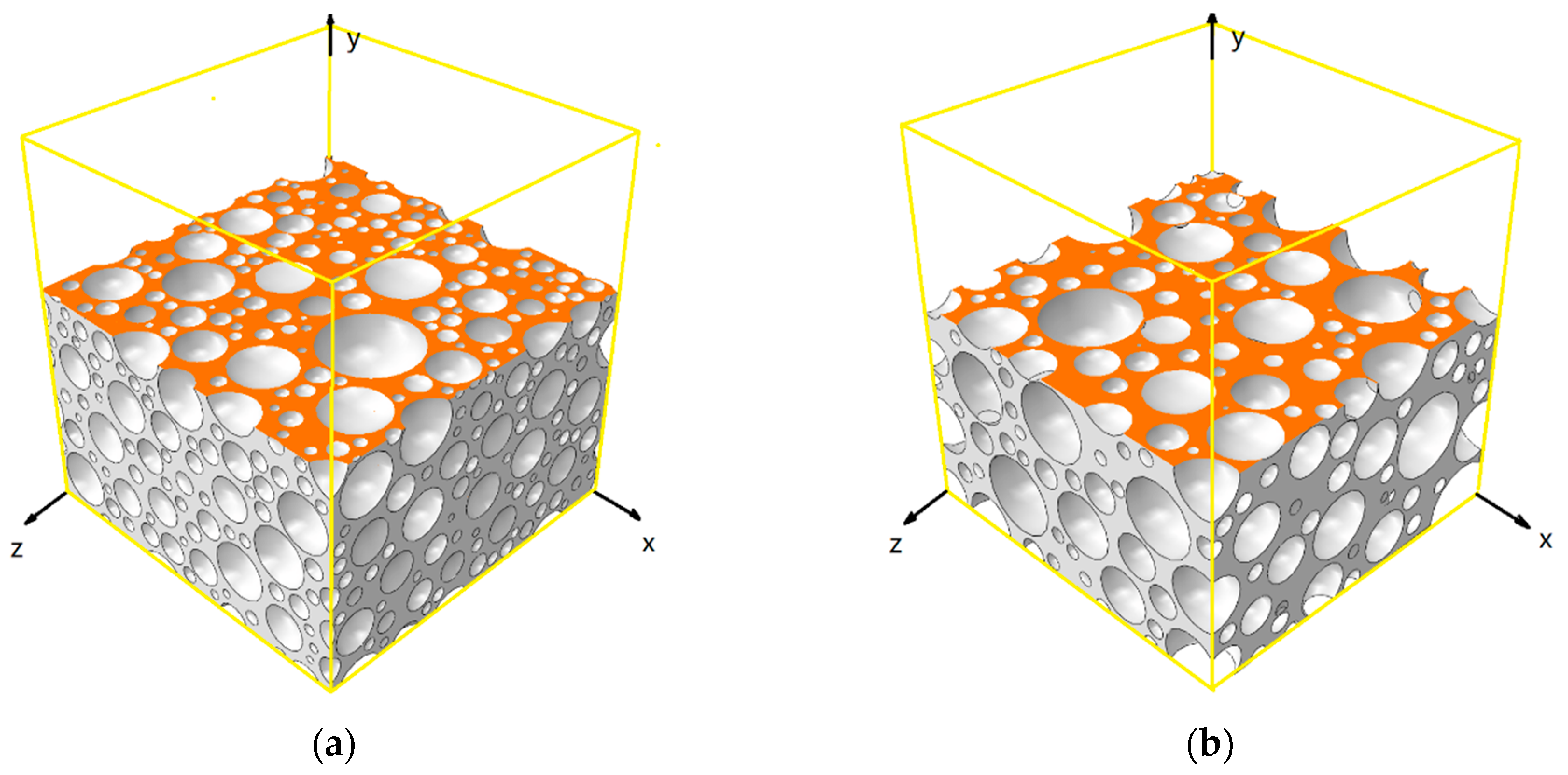
Figure 1. The random model: (a) Model 1 in Table 1, (b) Model 2 in Table 1, (c) Model 3 in Table 1, (d) Model 4 in Table 1, (e) Model 5 in Table 1, (f) Model 6 in Table 1, (g) Model 7 in Table 1, Kelvin model: (h) The RVE of the Kelvin model.
Applsci 13 08732 g001aApplsci 13 08732 g001b
Figure 2. The stress-strain curve of random model 1 and 3 in Table 1 with different element sizes.
Applsci 13 08732 g002
Figure 3. The stress-strain curves of Model 1 along the x, y, and z axis under uniaxial compression loading.
Applsci 13 08732 g003
Figure 4. The characteristic and principal stress-strain curves under uniaxial compression loading. Note: Point A is the yield point determined by 0.2% plastic strain offset in the characteristic stress-strain curve; Point B is the yield point determined by 0.2% plastic strain offset in the uniaxial stress-strain curve.
Applsci 13 08732 g004
Figure 5. The characteristic stress-strain curve under multiaxial load (−1.963:−3:−4). Note: Point A is the yield point determined by 0.2% plastic strain offset in the characteristic stress-strain curve.
Applsci 13 08732 g005
Figure 6. The yield surfaces are given with the 0.2% offset of the characteristic stress-strain curve method.
Applsci 13 08732 g006
Figure 7. The yield surfaces are given with the critical plastic dissipation energy method.
Applsci 13 08732 g007
Figure 8. Comparison of measured yield surfaces with predicted yield surfaces of the Kelvin model and random model using the yield definition method of critical plastic dissipation energy.
Applsci 13 08732 g008
Figure 9. The yield surfaces defined by the E c h based on the micro-scale.
Applsci 13 08732 g009
Figure 10. The yield surfaces defined by the E c h based on the micro-scale. Comparison of yield surfaces defined by the E c h and W of random model 1 with a relative density of 0.4.
Applsci 13 08732 g010
Figure 11. The relation of parameter A with k and cos 3 θ .
Applsci 13 08732 g011
Figure 12. The relation of parameter A with ρ 1 2 ν for different values of k: (a) k = 0, (b) k = −0.3, (c) k = −0.6, (d) k = −1, (e) k = −1.5, (f) k = −3.
Applsci 13 08732 g012aApplsci 13 08732 g012b
Figure 13. The energy values obtained with the plasticity models and the experiment of RVE models in Table 1 under uniaxial loading.
Applsci 13 08732 g013
Figure 14. The difference value between the energy values obtained with the plasticity models and the experiment of RVE models with 0.4 relate density under uniaxial loading.
Applsci 13 08732 g014
Figure 15. The yield surfaces of models with different inner structures determined by the corrected W c h .
Applsci 13 08732 g015
Table 1. The characteristic diameter D c h and characteristic shape anisotropy α c h of different models.
NumberRelative Density D c h / m m α c h
10.43.110
20.43.790
30.43.30.026
40.43.290.06
50.353.410.088
60.33.680.101
70.253.710.102
Table 2. Foam aluminum bulk material parameters.
Material ParameterValue
Elasticity modulus E/MPa72,400
Poisson’s ratio0.33
Plastic   modulus   E p /MPa77.8
Yield   strength   σ 0 /MPa140
Table 3. The number of elements in a random model with different element sizes.
Model NumberNumber of Element
Size 0.6 mmSize 0.4 mmSize 0.3 mmSize 0.25 mm
1121,478305,784585,765867,593
3104,871259,658457,528862,369
Table 4. The stress ratios used in the numerical simulations.
σ 1 σ 2 σ 3 k cos 3 θ
11.−2 −1
2−1−1 1
00−1−3−1
1−1.366−3.732−30
1−2−2−31
11−4−1.5−1
−0.134−1−1.8661−1.50
0−1−1−1.51
−1−1−2.5−1−1
−1−2.367−3.733−10
−1−4−4−11
−4−4−7−0.6−1
−1.9364−3−4−0.60.0534
−1−2−2−0.61
−3−3−4−0.3−1
−1−1.375−1.375−0.31
−1−1−10
Table 5. The relationship of related density and plastic dissipation energy per unit volume.
Related Density Plastic Dissipation Energy Per Unit Volume (×10−3 mJ/mm3)
KelvinModel 1Model 2Model 3Model 4Model 5Model 6Model 7
0.4360.6
0.222.8
0.4 57.348.139.731.5
0.35 21.4
0.3 20.1
0.25 15.7
Table 6. Comparison of E c h and W for the random model with a relative density of 0.4.
σ 1 σ 2 σ 3 E c h   ( J / mm 3 ) W (J/mm3)
00−10.038330.03373
1−1.366−3.7320.038330.03537
1−2−20.038330.03742
−1−1−40.038330.03381
−0.134−1−1.86610.038330.03714
0−1−10.038330.0355
−1−1−2.50.038330.03517
−1−2.367−3.7330.038330.03734
−1−4−40.038330.0363
−4−4−70.038330.03643
−1.9364−3−40.038330.03726
−1−2−20.038330.03689
−3−3−40.038330.03742
−1−1−10.038330.03776
Disclaimer/Publisher’s Note: The statements, opinions and data contained in all publications are solely those of the individual author(s) and contributor(s) and not of MDPI and/or the editor(s). MDPI and/or the editor(s) disclaim responsibility for any injury to people or property resulting from any ideas, methods, instructions or products referred to in the content.