Abstract
The use of delivery drones is currently hindered by the inability of transported objects to maintain a steady position, which can result from roll-, pitch-, and heave-induced vibrations. This paper proposes a novel parallel manipulator for stabilizing the platform of unmanned aerial vehicles. The proposed mechanism builds upon an existing study of a 3-SRR/SRU parallel stabilizing mechanism by incorporating the dynamical properties of the system into the control model. The resultant control technique is then applied to both the 3-RRS and 3-SRR mechanisms, and a comparative study is conducted to identify the most reliable stabilizer for regulating the platform’s orientation. The results demonstrate that the 3-SRR mechanism exhibits superior robustness and stability characteristics compared to the other two mechanisms. Additionally, the 3-SRR mechanism is controlled using artificial neural networks, which significantly improves the accuracy and stability of the system. Overall, this research presents a novel and effective solution for stabilizing the platform of unmanned aerial vehicles, with significant implications for the development of delivery drone technology.
1. Introduction
The use of drones across a multitude of industries, including military, delivery, monitoring, and agriculture, has become increasingly prevalent in recent years. One significant challenge faced by companies in these sectors is the limited capacity of traditional transportation infrastructure, particularly within urban areas, as the demand for commercial deliveries continues to escalate. In response, drone delivery systems have been proposed as a potential solution to alleviate traffic congestion by taking advantage of the vertical airspace above a city’s roadways while also addressing pressing environmental and noise pollution concerns [1]. Companies like Amazon and Google have, therefore, started looking for alternative delivery strategies—for instance, using unmanned aerial vehicles or autonomous drones [2]. In fact, autonomous drone delivery modes are anticipated to play a significant role in the future of the logistics sector, both for the last-mile delivery of small packages and for the delivery of fast food and restaurant meals. Domino’s Pizza, in collaboration with the New Zealand start-up Flirtey, has initiated trials for drone delivery services for pizzas and food [3]. Also, delivery robots have been increasingly adopted in various cities worldwide, mainly in response to customers’ COVID-19-related concerns about staying at home during lockdowns and the potential risks faced by human delivery personnel during the pandemic [3]. Recently, there has been a growing focus in research on the transportation of loads, which stands out as one of the most prevalent activities carried out with unmanned aerial vehicles [4,5]. However, to enable widespread drone use, significant changes need to be made to the current delivery-drone technology. For instance, when delivering food items such as pizza or hot syrup, it is crucial to isolate them from vibrations caused by heave, roll, and pitch movements. One solution to this problem is to utilize a stabilizing manipulator with three degrees of freedom (DOFs).
Serial manipulators (SMs) and parallel manipulators (PMs) are two primary divisions of robot manipulators. PMs have multiple limbs that share the payload capacity, providing a higher capacity than SMs. Moreover, PMs are better at precise positioning compared to their serial counterparts [6,7,8]. Recent studies have focused on developing and studying parallel manipulators for applications such as ship stabilization, wheelchair control, and helicopter landing aboard ships. Alkhedher et al. [9] utilized an inverted 6-DOF parallel manipulator as a stabilizer for any vehicle encountering path-bump variations. PMs with 2R1T motion, namely, two independent rotations and one translation, have been investigated as well. Zhan et al. [10] studied the forward kinematics of a 3-SPR (in this paper, P, R, S, and U stand for prismatic, revolute, spherical, and universal joints, respectively) wave compensation counteract mechanism and compared it to the 3-PSR mechanism for marine ships with dynamic positioning systems. Talke et al. [11] proposed a 3-PSR shipboard stabilization platform to mimic the fundamental DOFs of “roll, pitch, and heave” for wave replication to support the tethered unmanned aerial vehicles’ (UAV) winch payloads. Javadi et al. [12] studied the kinematics and dynamics of the 3-RRS mechanism for a torque-model-based PD controller to stop a disabled person who is using a typical electric wheelchair from tipping over. Tetik et al. [13] developed a mathematical model of the 3-RRS PM and performed position control over the physical model of the PM. Zhang et al. [14] proposed a kinematic control of a 3-SRR/SRU 3-DOF PM designed as a stabilization platform for helicopters landing aboard ships safely. Nevertheless, the dynamical model of the 3-SRR/SRU PM was not included in the control approach.
Despite its simplicity, proportional–integral–derivative (PID) control is frequently used to control the position and/or orientation of parallel manipulators [15,16]. When the PID parameters for the control object are set to their ideal values, the system outputs a response that is fairly close to the target value. Typically, the method of determining the PID parameters’ ideal values is called tuning, and it is often undertaken through trial and error, simulation, or systematic methods such as Ziegler–Nichols, ITAE, and robust PID tuning [17,18]. However, a significant shortcoming of these approaches is that PID parameters need to be manually adjusted anytime the system’s characteristics change. Changes in load, environment, or operating conditions make it difficult to fully automate the tuning procedure. On the other hand, manual tuning can be time consuming and may not always produce the best performance, especially in complicated dynamic systems [19]. To overcome this difficulty, there has been an increase in interest in creating automated tuning techniques and adaptive control schemes that can automatically modify the PID parameters in real time based on altering the system conditions. Although adaptive control techniques and automated tuning methods can substantially simplify the tuning process, they can still be time consuming and need significant computations [20,21]. Fuzzy logic control (FLC) is one of the techniques that can be used for the autotuning of PID controllers. In a fuzzy PID controller, human knowledge and expertise are used to design the fuzzy rules that determine the control action based on the system’s behavior and feedback [22]. There are several difficulties associated with fuzzy logic control, including high dependence on human knowledge and skill; fuzzy rules need to be updated over time, and there is no set method for creating fuzzy controllers [19]. On the other hand, robust nonlinear control techniques such as H-infinity loop shaping, sliding mode control, and so on [23,24,25,26] can be applied.
Recently, soft computing techniques such as neural networks have been successfully used in control systems. The use of artificial intelligence (AI) to replace the traditional PID controller can significantly simplify the tuning process and improve the overall performance and robustness of the control system [27,28,29]. Ghoniem et al. [30] replaced a PID controller with a neural network in order to control a new low-cost semi-active vehicle suspension system, and it proved to have good accuracy in terms of vibration reduction and response time. Rahimi et al. [31] presented a 3-DOF delta robot trajectory-tracking control using an online neural network self-tuned inverse dynamic controller. Nguyet et al. [32] proposed an enhanced PID controller with an artificial neural network (ANN) to increase the position control efficiency of a 2-DOF robotic arm. The controller has shown robust and flexible results.
Although control approaches have been proposed for stabilizing UAV platform mechanisms, most existing works rely on classical control techniques. Furthermore, previous studies lack a comparative analysis of the performance of different stabilizing mechanisms, which limits insights into the impact of robot architecture on stabilized motion. This paper aims to address these gaps by proposing a parallel mechanism for UAV platform stabilization, utilizing modern control techniques for mechanism control. A comparative study is conducted on three different parallel manipulators. Initially, the 3-SRR/SRU PM is investigated, and a control technique based on both kinematical and dynamical models is developed, extending previous works. A new control strategy is proposed, which significantly improves the output values. The proposed control strategy is then applied to the 3-RRS PM, and the resulting motion of the moving plate is examined and compared with the 3-SRR/SRU PM. Based on further investigation of the results, a 3-SRR PM is proposed, which better addresses the stabilization problem of the moving platform. Additionally, the control of the 3-SRR PM is enhanced by incorporating an artificial neural network (ANN) to accurately predict output values while accommodating input changes, overcoming the drawbacks of tuning PID control.
2. Model Identification of 3-SRR/SRU
2.1. Mathematical Model
In this section, the mathematical model devised by Zhang et al. [14] for the 3-SRR/SRU PM is recapitulated, where R designates an actuated revolute joint. The 3-SRR/SRU PM, depicted in Figure 1, was investigated as a stabilization platform for helicopters landing aboard ships safely. It consists of three SRR limbs, , , and , in addition to one passive SRU limb, . The moving plate has 2R1T 3-DOF motion [14], namely two independent rotations in addition to one translation. Points and () denote the intersection between the moving plate and the base, respectively, and the joints implemented on them. Points , , and express the centers of the moving plate, the base, and the ship, respectively, the base being installed on the ship. The relative position of the base with respect to the ship is expressed by ,, and , namely, the coordinates of with respect to .
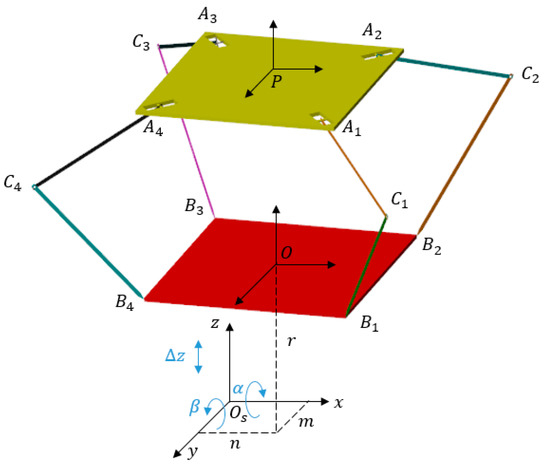
Figure 1.
CAD model of 3-SRR/SRU parallel mechanism.
The motion of the ship is represented by heave , roll , and pitch in the reference frame as illustrated in Figure 1. The moving plate and the base both have a square cross-section, as seen from the top. Thus, let denote the distance between the center of the base, , and each of points (). Accordingly, the coordinates of relative to the ship’s motion are as follows (in Equation (1), operators “” and “” represent the trigonometric functions “sin” and “cos”, respectively):
Similarly, let express the distance between center of the moving plate and each of points (). In addition, let represent the initial distance between the moving plate and the base. The initial coordinates of points () with respect to can be written as follows:
is the initial distance between the two plates, and and present the distance between the center frame O and the selected A (i = 1, 2, 3, and 4). Recalling that the initial coordinates of each A with respect to Ob can be written as follows [14]:
2.2. Existing Control Strategy
In each limb, let and , (). Zhang et al. [14] designed a kinematic control strategy that consists of calculating the desired angles , () at the actuated joints, for which the moving plate returns to its initial position with every change in the ship motion. Using the cosine law, angles are formulated as follows:
2.3. Simscape Modeling and Validation
The Simscape model presented in Figure 2 was implemented based on the CAD model shown in Figure 1 in order to validate the kinematic analysis by using the design parameters described in [14] and the same inputs as well.
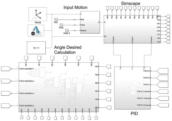
Figure 2.
Simscape model.
A Simulink block is utilized to calculate the desired angles based on the coordinates of points obtained from the transform sensor at each instant. The coordinates of points are initialized with their numerical values based on the design parameters. Figure 3 presents a comparison of angles - (), obtained from the Simscape model in Figure 2, and the values -Zhang et al. 2014, (), of the same angles digitized from [14]. It is noteworthy that the figures displaying and were omitted because of space limitations, but their results align with those presented for and .
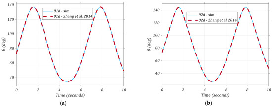
Figure 3.
Comparison between Simscape results and results from Zhang et al. [14] for (a) and (b) .
The comparison depicted in Figure 3 shows strong alignment between the entities being compared, indicating a successful validation of the Simscape model using the kinematic equations.
3. PID Control of the Dynamical Model
The study presented here extends that of [14] by incorporating the dynamics of the 3-SRR/SRU PM, as the latter was limited to the kinematical model only. To validate the enhanced accuracy achieved through the incorporation of mechanism dynamics, AISI steel 308 is assigned for the different parts of the PM. It is important to note that AISI steel 308 holds significant prominence in the industry because of its wide usage. Figure 4 shows a comparison among the actual output angles from Simscape and from [14] -, and -Zhang et al. 2014, respectively, and the desired angles for the dynamical model for and .
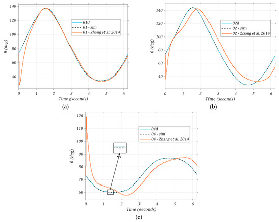
Figure 4.
Comparison among the output angles from Simscape, -, and from Zhang et al. 2014 [14], respectively, and the desired angles for (a) , (b) , and (c) after incorporating the dynamical model.
The simulation results obtained from the Simscape dynamical model exhibit a significant improvement, showcasing minimal deviations between the desired angles and the actual output angles. These deviations are visually depicted through the scaled capture included in Figure 4c, providing a clear representation of the slight variations observed. Conversely, the output angles obtained from [14] exhibit inadequate tracking of the desired angles, with notable delays observed specifically in angles 2 and 4. Additionally, it is worth noting that all the tracking curves in [14] exhibit an impulse at the beginning, which differs from the tracking curves obtained from our model. This precise alignment can be attributed to the incorporation of both kinetics and kinematics in our present model, thus enhancing its accuracy and reliability. Additionally, a fine tuning of the PID-controller gains was performed in Matlab, optimizing the controller’s performance. The synergistic effect of these factors contributed to the remarkable agreement between the desired and actual output values.
3.1. 3D Simulation
Zhang et al. [14] showed the desired curve for angle but did not display the actual angle values. Simscape is a powerful simulation tool that includes a mechanics explorer feature, enabling users to visualize and analyze the behavior of 3D Simscape models in real time. This feature provides an intuitive workspace for monitoring the simulation results at any point during the simulation. While watching the 3D simulation, at the instant when , , and were attained, it was observed that the moving plate was not stabilized correctly, as shown in Figure 5.
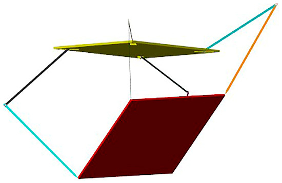
Figure 5.
Position of the upper moving plate of the 3-SRR/SRU when , , and .
Additionally, the simulation data inspector revealed that the actual angle, represented by , of the passive joint within the SRU limb is incapable of tracking its desired value in any given scenario, as depicted in Figure 6.
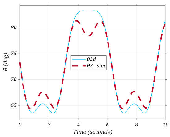
Figure 6.
Comparison between the desired and actual values of using the existing strategy.
As a consequence of this issue, the dynamical model showcases sinusoidal fluctuations in the and coordinates of points , (). The positional variation of point is illustrated in Figure 7. Although the figures illustrating the variations for , , and were not included because of limited space, their results align consistently with those presented for .
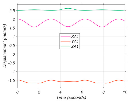
Figure 7.
Variation in the position of point on the moving plate.
3.2. Proposed Control Strategy
The existing control strategy [14] consists of blocking the motion of points in all directions, , , and and accordingly calculating the desired angles at the actuators using Equation (3). However, this approach encounters challenges in maintaining the positions of points at their initial values, as it fails to prevent the fluctuations in the and coordinates, which subsequently lead to errors in the position. This inadequacy is clearly illustrated in Figure 5, which highlights the failure in maintaining the horizontal position of the platform and its stability.
To overcome this issue, an alternative solution is proposed here and consists of allowing variations in the and positions. This solution involves computing the desired angles at the actuators using Equation (3) by considering the and positions at each instant, while keeping the initial value of the coordinate constant. Implementing this solution has proven effective in stabilizing the moving plate, as evidenced by the results presented in Figure 8.
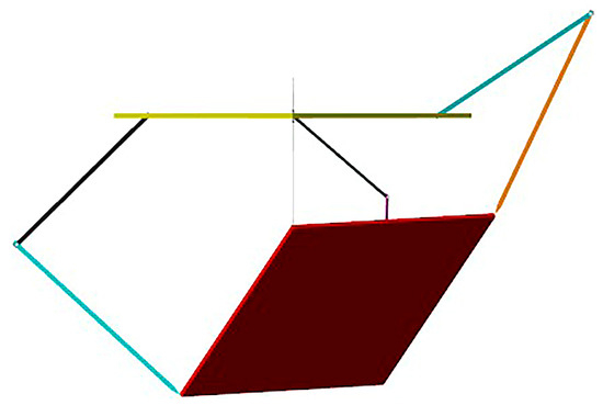
Figure 8.
Position of the upper moving plate of 3-SRR/SRU when , , and using the proposed strategy.
In summary, the proposed solution acknowledges that small fluctuations in the and coordinates can be tolerated to some extent. However, it emphasizes the importance of effectively controlling variations in the position to ensure the stability of the platform.
Furthermore, with the implementation of the proposed solution, the actual angle exhibited precise tracking of the newly calculated desired angle , as clearly demonstrated in Figure 9.
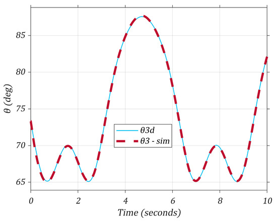
Figure 9.
Comparison of the desired and actual values of angle using the proposed strategy.
Nonetheless, the proposed solution has a minor drawback, which is a slight increase in variation in the x and y positions compared to the previous approach, as depicted in Figure 10.
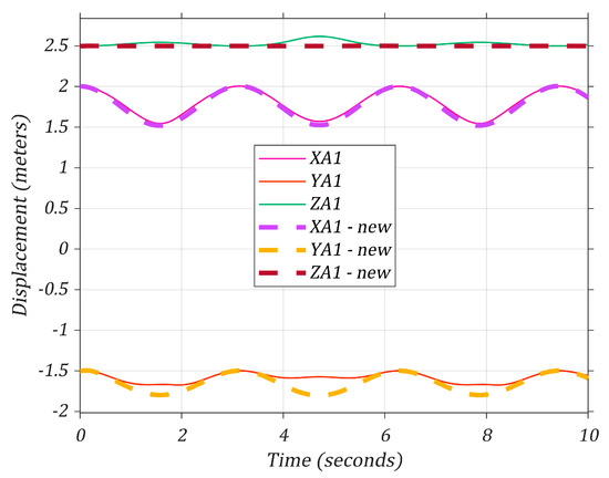
Figure 10.
Coordinates of using the previous approach and the new approach.
The results demonstrate that incorporating the resulting and positions at each instant in the control strategy yields superior outcomes and effectively resolves the dynamical issue at hand.
4. Alternative Solutions for UAV Stabilizing Mechanism
4.1. 3-RRS PM
To achieve a 3-DOF 2R1T (two rotational and one translational) motion [12], an additional parallel mechanism known as the 3-RRS mechanism is being considered. This mechanism consists of a base and a moving plate in the shape of an equilateral triangle. The angle between joint 1 and joint 2 is set at 120° in the horizontal plane, as illustrated in [13].
To ensure the accuracy of the kinematics and rotation matrices, validation has been conducted between the formulated results and Simscape. Consequently, the 3-RRS mechanism has been seamlessly integrated into MATLAB without the need for manual kinematics formulation. The control of the 3-RRS mechanism relies on the angle , which is between the upper plate and the upper arms, which means the motor is assembled upward between the base plate and arm , thereby acting as an active revolute joint, as shown in Figure 11. This figure depicts the geometric arrangement of one of the kinematic chains of the 3-RRS parallel mechanism.
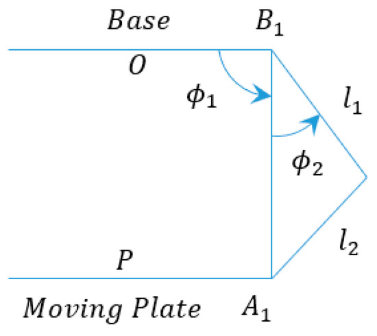
Figure 11.
Schematic representation of RRS limb.
A Simulink block was implemented to calculate the desired angle , which is the summation of and by using the coordinates of point , the center of the base plate at each time instant. The scales used in this simulation are representing the diameter of the base plate where points are located, and representing the diameter of the moving plate on which the coordinates are located. Additionally, the parameters and are utilized. By applying the proposed control strategy, remarkable progress was achieved in stabilizing the moving plate, as illustrated in Figure 12.
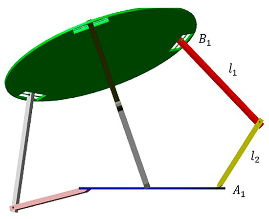
Figure 12.
3D Simulation of the 3-RRS PM when and using the proposed strategy.
The monitoring of the system has revealed the robustness of the moving plate when utilizing the proposed strategy. However, it is important to note that this strategy does introduce a higher variation in the and coordinates, which can be attributed to the distribution of the joints within the 3-RRS PM. Furthermore, to further investigate the effects of this variation, a similarly scaled 3-SRR/SRU parallel mechanism was implemented. A comparison of the results for both mechanisms is presented in Figure 13, highlighting the significant variation observed in the 3-RRS PM.
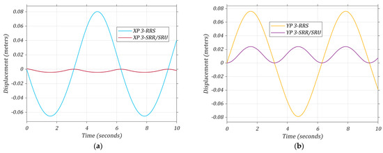
Figure 13.
Variation of the coordinates of the moving-plate center P for 3-RRS and 3-SRR/SRU PMs using the proposed strategy: (a) component; (b) component.
4.2. Proposed Mechanism: 3-SRR PM
Through a thorough comparison of the results obtained from the 3-SRR/SRU PM and the 3-RRS PM, it becomes evident that the positioning of the spherical joint significantly influences the system’s behavior. Depending on whether the joint is assembled on the moving plate or the base plate, different outcomes are observed. To further investigate this aspect, the same mechanism with reversed joint configurations was implemented. This PM comprises a base and a moving platform in the form of an equilateral triangle. It consists of three identical limbs with SRR kinematic chain structures, offering an alternative configuration.
When employing the existing strategy, which is based on fixed coordinates of , variations are observed in all directions, including the z directions. However, the implementation of the proposed strategy proves successful in restoring all the z coordinates of to their initial positions, although with a slight increase in the and coordinates. These observations are clearly illustrated in Figure 14. The findings highlight the effectiveness of the proposed strategy in maintaining the desired -coordinate positions of while managing the trade-off between variations in the and coordinates.
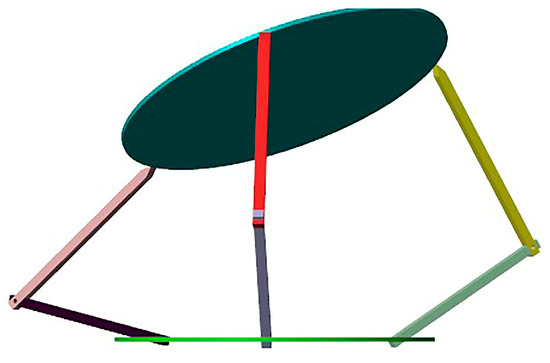
Figure 14.
3D simulation of the 3-SRR PM when and using the proposed strategy.
4.3. Comparison of 3-SRR and 3-SRR/SRU PMs
All three mechanisms have demonstrated robust performance. However, in the case of the 3-RRS PM, the stabilization of the plate necessitated movement in the and directions in a free manner. Consequently, a comparison was conducted solely between the translational motion of the moving plate for the 3-SRR/SRU PM and the 3-SRR PM, both utilizing the proposed strategy. This comparative analysis provides valuable insights into the effectiveness and characteristics of translational motion for these two mechanisms under the given strategy.
The translational distance in the 2D plane for each mechanism is calculated using the Pythagorean theorem:
For the 3-SRR/SRU:
For the 3-SRR:
The analysis of the graphs presented in Figure 15, as well as the calculations based on Equations (7) and (8), reveal that the 3-SRR PM undergoes a translational motion of approximately 16.77 mm, while the 3-SRR/SRU PM experiences a translational motion of around 24.31 mm. It is noteworthy that both mechanisms effectively stabilize the plate in the z direction.
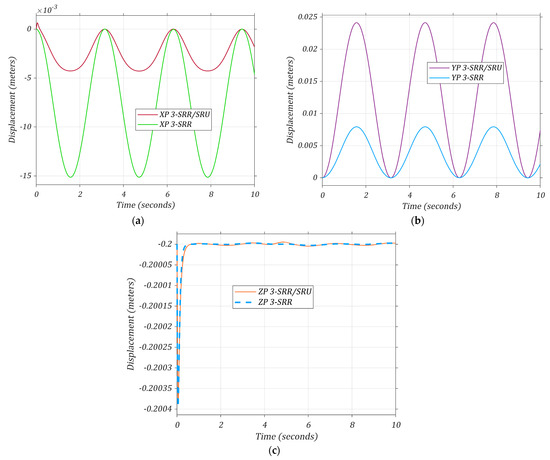
Figure 15.
Variations of the coordinates of the moving-plate center for 3-SRR/SRU and 3-SRR PMs using the proposed strategy: (a) component; (b) component; (c) component.
These results demonstrate that both mechanisms successfully achieve the desired goal of plate stabilization, with only a negligible drawback. The 3-SRR PM, with its lesser translational motion, offers the advantage of easier assembly by avoiding the use of universal joint assembly. Consequently, for the remainder of the paper, the focus will be on the utilization and analysis of the 3-SRR mechanism, which proves to be a suitable choice for the intended purpose.
5. Artificial Neural Network
5.1. Obtaining Design Parameters
In this study, the 3-SRR PM is chosen for UAV stabilization purposes. To meet the specific requirements of the application, design parameters need to be established. The M200 V2 DJI drone [33] suggests a maximum tilt angle of in S mode. Therefore, the design parameters will be determined with this constraint in mind. Additionally, the PM should be capable of operating under vibrations in the heave direction within the range of −0.02 m to 0.02 m. Assume that , ,, and .
A trial-and-error approach is employed using a Simulink block implemented in MATLAB based on Equation (3). By applying maximum inputs of , , and , the value of is determined to be , thus achieving the desired goal.
5.2. Neural Network
PID controllers exhibit a notable limitation in their robustness when encountering changes in system parameters. As a result, they are unable to achieve perfect stabilization across various inputs and frequencies, necessitating the need to retune the PID parameters whenever such changes occur. Therefore, the purpose of this section is to replace the PID control system with a trained artificial neural network (ANN) and then examine the system’s responsiveness to various excitations. Initially, the error signal entering the PID will serve as the input data, while the corresponding output data from the PID will be used as the target output data for training the ANN. Data collection is performed at different frequencies and with varying roll-and-pitch angles to capture the system’s behavior under diverse conditions. It is important to highlight that each run necessitates careful fine tuning of the PID parameters to achieve the optimal response.
For training the ANN, the Levenberg–Marquardt algorithm is employed, and the network architecture consists of two layers of feed-forward connections. Figure 16 depicts a visual representation of network architecture, showcasing a two-layer feed-forward configuration. This configuration consists of a hidden layer with 10 neurons, characterized by the sigmoid activation function. The output layer, depicted in Figure 16 as well, employs a linear activation function with one neuron making it suitable for regression tasks. This visual representation provides an overview of the structure of the neural network and the activation functions utilized in each layer. This architecture enables accurate regression for the desired control tasks. Collected data from the PID is divided into three sets: 70% for training the neural network, 15% for verification to ensure the legitimacy of the training data, and the remaining 15% for testing the finalized neural network.
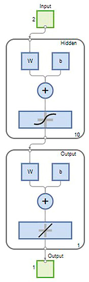
Figure 16.
Structure of the artificial neural network.
After training the ANN, it became evident that the regression model achieved a low regression value R, indicating a poor fit between the predicted and actual values. This outcome is depicted in Figure 17, where the regression line deviates significantly from the ideal fit. To further analyze the performance of the trained neural network, the data were loaded into the regression learner application. Figure 18 illustrates a comparison between the output of the PID controller and the predictions of the trained neural network in relation to error . It is observed that the neural fitting is unable to accurately follow the circular shape because of the error’s fluctuation over time.
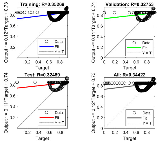
Figure 17.
Regression plot for the first input.
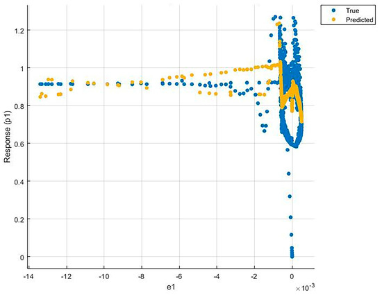
Figure 18.
Comparison of the PID output and the predicted output of the trained neural network with respect to error .
This discrepancy indicated a lack of relevant data in the input. To address this, time data were collected and incorporated into the input as a representation of frequency. The updated dataset, including the time input, was then loaded into the regression learner application in MATLAB.
Subsequently, the new data, along with the new added time input, were utilized to retrain the neural network using the regression learner application. The neural network’s predicted output exhibited a much-improved fit to the error, even successfully capturing the peculiar shapes resulting from the inclusion of the time input, as shown in Figure 19. Notably, the training results showed a significantly higher R-squared value of 0.9 and a reduced mean-squared error (MSE) of 0.00099, showcasing the enhanced performance of the revised model.
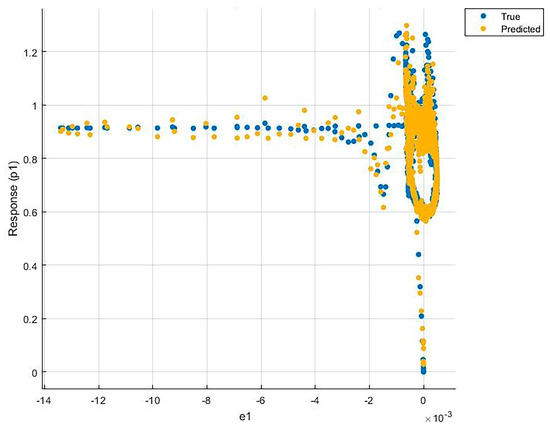
Figure 19.
Comparison of the PID output and the predicted output of the improved neural network with respect to error .
To integrate the trained model into Simulink, time was added as a column in the input matrix for each error of the three PID controllers. The trained block was exported from the neural fitting program to Simulink, where further training was conducted. The data for neural networks 1, 2, and 3 have predictor responses. The predictors comprised two columns with 3347 variables representing error and time, while the responses consisted of a single column with 3347 variables representing the PID output.
Graphs displayed in Figure 20 showcased a perfect fit between the network’s output and target values for the three controllers, as evidenced by high overall regression R values of 0.97, 0.995, and 0.9819, respectively.
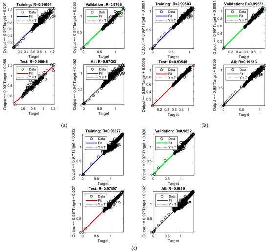
Figure 20.
Regression plot for outputs: (a) 1; (b) 2; (c) 3.
5.3. Results from ANN
To assess the performance of the neural network in conjunction with Simscape, the system was subjected to the maximum tilt angles and vibrations in heave. These tests were conducted at the maximum tilt angles of the drone and at different frequencies, as shown in Equations (9)–(11), to evaluate the neural network’s effectiveness across different operating conditions.
The results presented in Figure 21 and Figure 22 demonstrate the remarkable achievement of the trained neural network. It successfully fulfills the mission of achieving perfect stabilization across various inputs and frequencies, without the need for retuning the PID parameters. The neural network’s predictions, based on the extensive dataset provided during training, enable precise and effective control of the system. This underscores the power and efficiency of the neural network approach in achieving robust and reliable stabilization.
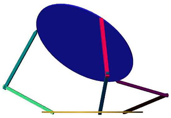
Figure 21.
Three-dimensional simulation of the 3-SRR PM controlled by a neural network.
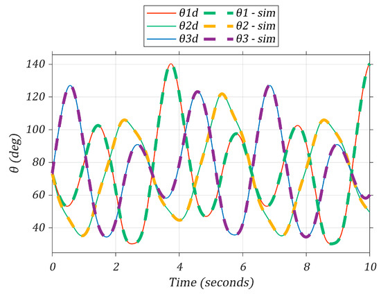
Figure 22.
Comparison of and - () for the 3-SRR PM controlled by a neural network.
6. Conclusions and Future Work
In this study, the initial phase involved the validation of the kinematic properties of the 3-SRR/SRU parallel mechanism using Simscape modeling. Building upon this, an enhanced control approach was developed by incorporating the dynamical properties of the mechanism.
A comparative study was conducted by applying the enhanced control method to other 3-DOF parallel manipulators, namely the 3-RRS and 3-SRR parallel mechanisms, with the objective of identifying an effective stabilizer for the control of the platform orientation of unmanned aerial vehicles. Notably, the PID control implemented in this study outperformed previously published data, exhibiting precise tracking of the desired output with minimal delay. Among the three manipulators compared, the 3-SRR mechanism emerged as the most capable of achieving the desired robust stabilizing outcome. Furthermore, the challenge of adjusting PID gains was addressed through the incorporation of artificial neural networks within the 3-SRR parallel mechanism, showcasing improved controller precision and stability. Future work entails the experimental implementation of the 3-SRR parallel manipulator using the validated control strategy.
Author Contributions
Conceptualization, O.M. and S.A.; methodology, M.H.C.; software, M.H.C.; validation, E.G.H., M.H.C., O.M., and S.A.; formal analysis, M.H.C.; investigation, E.G.H., M.H.C., O.M., and S.A.; resources, E.G.H., O.M., and S.A.; data curation, E.G.H., O.M., and S.A.; writing—original draft preparation, M.H.C.; writing—review and editing, E.G.H., O.M., and S.A.; visualization, E.G.H., M.H.C., O.M., and S.A.; supervision, E.G.H., O.M., and S.A. All authors have read and agreed to the published version of the manuscript.
Funding
This research received no external funding.
Institutional Review Board Statement
Not applicable.
Informed Consent Statement
Not applicable.
Data Availability Statement
The data presented in this paper is available upon request by contacting the corresponding author.
Conflicts of Interest
The authors declare no conflict of interest.
References
- Borghetti, F.; Caballini, C.; Carboni, A.; Grossato, G.; Maja, R.; Barabino, B. The Use of Drones for Last-Mile Delivery: A Numerical Case Study in Milan, Italy. Sustainability 2022, 14, 1766. [Google Scholar] [CrossRef]
- Merkert, R.; Bushell, J. Managing the Drone Revolution: A Systematic Literature Review into the Current Use of Airborne Drones and Future Strategic Directions for Their Effective Control. J. Air Transp. Manag. 2020, 89, 101929. [Google Scholar] [CrossRef] [PubMed]
- Benarbia, T.; Kyamakya, K. A Literature Review of Drone-Based Package Delivery Logistics Systems and Their Implementation Feasibility. Sustainability 2022, 14, 360. [Google Scholar] [CrossRef]
- Urbina-Brito, N.; Guerrero-Sánchez, M.-E.; Valencia-Palomo, G.; Hernández-González, O.; López-Estrada, F.-R.; Hoyo-Montaño, J.A. A Predictive Control Strategy for Aerial Payload Transportation with an Unmanned Aerial Vehicle. Mathematics 2021, 9, 1822. [Google Scholar] [CrossRef]
- Guerrero-Sánchez, M.E.; Hernández-González, O.; Valencia-Palomo, G.; Mercado-Ravell, D.A.; López-Estrada, F.R.; Hoyo-Montaño, J.A. Robust IDA-PBC for under-Actuated Systems with Inertia Matrix Dependent of the Unactuated Coordinates: Application to a UAV Carrying a Load. Nonlinear Dyn. 2021, 105, 3225–3238. [Google Scholar] [CrossRef]
- Patel, Y.D.; George, P.M. Parallel Manipulators Applications—A Survey. Mod. Mech. Eng. 2012, 2, 57–64. [Google Scholar] [CrossRef]
- Wang, Y.; Lyu, C.; Liu, J. Kinematic Analysis and Verification of a New 5-DOF Parallel Mechanism. Appl. Sci. 2021, 11, 8157. [Google Scholar] [CrossRef]
- Wang, L.; Wang, D.; Wu, J. Dynamic Performance Analysis of Parallel Manipulators Based on Two-Inertia-System. Mech. Mach. Theory 2019, 137, 237–253. [Google Scholar] [CrossRef]
- Alkhedher, M.; Younes, T.; Mohamad, O.; Ali, U. Adaptive 6 DOF Self-Balancing Platform for Autonomous Vehicles. Int. J. Comput. Digit. Syst. 2020, 9, 69–75. [Google Scholar] [CrossRef]
- Zhan, Y.; Tian, H.; Xu, J.; Wu, S.; Fu, J. A Novel Three-SPR Parallel Platform for Vessel Wave Compensation. J. Mar. Sci. Eng. 2020, 8, 1013. [Google Scholar] [CrossRef]
- Talke, K.; Drotman, D.; Stroumtsos, N.; de Oliveira, M.; Bewley, T. Design and Parameter Optimization of a 3-PSR Parallel Mechanism for Replicating Wave and Boat Motion. In Proceedings of the 2019 International Conference on Robotics and Automation (ICRA), Montreal, QC, Canada, 20–24 May 2019; IEEE: New York, NY, USA, 2019; pp. 7955–7961. [Google Scholar]
- Javadi, M.; Afzalpour, N.; Taayemeh, P.J.; Khorsandijou, S.M. Wheelchair Stabilization by the Control of a Spatial 3-RRS Mechanism. Iran. J. Mech. Eng. Trans. ISME 2016, 17, 84–100. [Google Scholar]
- Tetik, H.; Kalla, R.; Kiper, G.; Bandyopadhyay, S. Position Kinematics of a 3-RRS Parallel Manipulator. In ROMANSY 21—Robot Design, Dynamics and Control; Parenti-Castelli, V., Schiehlen, W., Eds.; CISM International Centre for Mechanical Sciences, Courses and Lectures; Springer International Publishing: Cham, Switzerland, 2016; Volume 569, pp. 65–72. ISBN 978-3-319-33713-5. [Google Scholar]
- Zhang, B.; Shang, W. Kinematic Control of a 3-DOF Parallel Stabilization Platform. In Proceedings of the 33rd Chinese Control Conference, Nanjing, China, 28–30 July 2014; IEEE: New York, NY, USA, 2014; pp. 8287–8292. [Google Scholar]
- Bennet, S. A Brief History of Automatic Control. IEEE Control Syst. 1996, 16, 17–25. [Google Scholar] [CrossRef]
- Ang, K.H.; Chong, G.; Li, Y. PID Control System Analysis, Design, and Technology. IEEE Trans. Control Syst. Technol. 2005, 13, 559–576. [Google Scholar] [CrossRef]
- Ziegler, J.G.; Nichols, N.B. Optimum Settings for Automatic Controllers. J. Dyn. Syst. Meas. Control 1993, 115, 220–222. [Google Scholar] [CrossRef]
- Portillo, J.; Marcos, M.; Orive, D.; López, F.; Pérez, F. PID_ATC: A Real-Time Tool for PID Control and Auto-Tuning. IFAC Proc. Vol. 1998, 31, 41–46. [Google Scholar] [CrossRef]
- Lee, Y.-S.; Jang, D.-W. Optimization of Neural Network-Based Self-Tuning PID Controllers for Second Order Mechanical Systems. Appl. Sci. 2021, 11, 8002. [Google Scholar] [CrossRef]
- Starr, K.D.; Petersen, H.; Bauer, M. Control Loop Performance Monitoring—ABB’s Experience over Two Decades. IFAC-Pap. 2016, 49, 526–532. [Google Scholar] [CrossRef]
- Berner, J.; Soltesz, K.; Hägglund, T.; Åström, K.J. An Experimental Comparison of PID Autotuners. Control Eng. Pract. 2018, 73, 124–133. [Google Scholar] [CrossRef]
- Zadeh, L.A. Fuzzy Sets. Inf. Control 1965, 8, 338–353. [Google Scholar] [CrossRef]
- Mokhiamar, O.; Abe, M. Experimental Verification Using a Driving Simulator of the Effect of Simultaneous Optimal Distribution of Tyre Forces for Active Vehicle Handling Control. Proc. Inst. Mech. Eng. Part D Automob. Eng. 2005, 219, 135–149. [Google Scholar] [CrossRef]
- Davidson, R.A.; Ushakumari, S. H-Infinity Loop-Shaping Controller for Load Frequency Control of a Deregulated Power System. Procedia Technol. 2016, 25, 775–784. [Google Scholar] [CrossRef]
- Amine, S.; Mokhiamar, O. A Study of Stability and Power Consumption of Electric Vehicles Using Different Modern Control Strategies. Alex. Eng. J. 2019, 58, 1281–1290. [Google Scholar] [CrossRef]
- Darwiche, M.; Mokhiamar, O. SVR Approach for Predicting Vehicle Velocity for Comfortable Ride While Crossing Speed Humps. Alex. Eng. J. 2022, 61, 6119–6128. [Google Scholar] [CrossRef]
- Jung, S.; Kim, S.S. Control Experiment of a Wheel-Driven Mobile Inverted Pendulum Using Neural Network. IEEE Trans. Control Syst. Technol. 2008, 16, 297–303. [Google Scholar] [CrossRef]
- Sun, Q.; Du, C.; Duan, Y.; Ren, H.; Li, H. Design and Application of Adaptive PID Controller Based on Asynchronous Advantage Actor–Critic Learning Method. Wirel. Netw. 2021, 27, 3537–3547. [Google Scholar] [CrossRef]
- Danh, N.C. Neural Networks Application for the Data of PID Controller for Acrobot. Sci. World J. 2022, 2022, e9162352. [Google Scholar] [CrossRef]
- Ghoniem, M.; Awad, T.; Mokhiamar, O. Control of a New Low-Cost Semi-Active Vehicle Suspension System Using Artificial Neural Networks. Alex. Eng. J. 2020, 59, 4013–4025. [Google Scholar] [CrossRef]
- Rahimi, S.; Jalali, H.; Hairi Yazdi, M.R.; Kalhor, A.; Tale Masouleh, M. Design and Practical Implementation of a Neural Network Self-Tuned Inverse Dynamic Controller for a 3-DoF Delta Parallel Robot Based on Arc Length Function for Smooth Trajectory Tracking. Mechatronics 2022, 84, 102772. [Google Scholar] [CrossRef]
- Minh Nguyet, N.T.; Ba, D.X. A Neural Flexible PID Controller for Task-Space Control of Robotic Manipulators. Front. Robot. AI 2023, 9, 975850. [Google Scholar] [CrossRef]
- Matrice 200 Series V2—Product Information—DJI. Available online: https://www.dji.com/global/matrice-200-series-v2/info (accessed on 19 July 2023).
Disclaimer/Publisher’s Note: The statements, opinions and data contained in all publications are solely those of the individual author(s) and contributor(s) and not of MDPI and/or the editor(s). MDPI and/or the editor(s) disclaim responsibility for any injury to people or property resulting from any ideas, methods, instructions or products referred to in the content. |
© 2023 by the authors. Licensee MDPI, Basel, Switzerland. This article is an open access article distributed under the terms and conditions of the Creative Commons Attribution (CC BY) license (https://creativecommons.org/licenses/by/4.0/).