Estimation of Time-Series Forest Leaf Area Index (LAI) Based on Sentinel-2 and MODIS

Abstract

The LAI is a key parameter used to describe the exchange of material and energy between soil, vegetation and the atmosphere. It has become an important driving datum in the study of carbon and water cycle mechanism models at many regional scales. In order to obtain high temporal resolution and high spatial resolution LAI products, this study proposed a method to combine the high temporal resolution of MODIS LAI products with the high spatial resolution of Sentinel-2 data. The method first used the LACC algorithm to smooth the LAI time-series data and extracted the normalized growth curve of the MODIS LAI of forest and used this curve to simulate the annual variation of the LAI. Secondly, it estimated the LAI at the period of full leaf spread based on the traditional remote sensing statistical model and Sentinel-2 remote sensing data as the maximum value of the forest LAI in the study area and used it to control the LAI growth curve. Finally, the time-series LAI data set was created by multiplying the maximum LAI by the normalized forest LAI growth curve. The results indicate that: (1) the remote sensing statistical estimation model of LAI was developed using the atmospherically resistant vegetation index ARVI ($R^2$ = 0.494); (2) the MODIS LAI normalized growth curve keeps a good level of agreement with the actual variation. This study provides a simple and efficient method for obtaining effective time-series forest LAI data for the scope of small- and medium-sized areas.

1. Introduction

The forest ecosystem is the main component of the terrestrial ecosystem [1,2]. Estimating the distribution and change of carbon storage in forest ecosystems is helpful for understanding the relationship between carbon sources and sinks [3,4,5]. The leaf area index is an important parameter for describing vegetation growth and one of the main parameters in ecological and climate models. It is defined as the sum of the one-sided area of green leaves per unit ground area [6,7]. The leaf area index is closely related to ecophysiological processes such as photosynthesis, transpiration, respiration and the productivity of vegetation [8,9,10,11]. It is an essential driving parameter in the carbon and water cycle of forest ecosystems at regional and global scales [12,13]. The time-series LAI characterizes the growth dynamics of vegetation, and obtaining the regional time-series LAI becomes an important data preparation step in the study of carbon and water cycle mechanism models at the regional scale [14,15]. How to quickly obtain a high spatial-temporal resolution sequence LAI has become a research focus.

At present, the estimation of the regional scale LAI mainly adopts the remote sensing inversion method [16,17], which is divided into two types of models—the statistical estimation model and the physical inversion model—according to whether it involves physical physiological processes. Physical inversion models [18,19,20] have clear physical meaning and require the input of the biochemical and structural parameters of leaves. They also have the shortcomings of large uncertainty, large computation and time consumption. Statistical estimation models [21,22,23,24] estimate the leaf area index by establishing linear or nonlinear relationships between the LAI and vegetation index, which have the advantages of few parameters and easy implementation. They are often applied to LAI estimation in smaller areas [25,26,27,28].

At present, a number of world-wide LAI products have been produced from many different types of satellite remote sensing data [29,30]. These products use multifarious methods for retrieval and have their own spatio-temporal resolutions. Table 1 lists the major LAI products in the world. It can be seen from Table 1 that the MODIS LAI has the highest spatial-temporal resolution (4 days, 500 m) in the system that is still running. Because of frequent clouds and other factors, the existing LAI products may be provided with anomalous time-series characteristics. In order to break through these difficulties, a few reconstruction methods, according to the principles of the statistical filtering and the data assimilation, have been put forward [31,32,33]. The reconstruction method based on the dynamic change mechanism model can restructure time-series LAI data by attaching additional data [34]. By attaching the radiative transfer model to the dual logic LAI time model, the time-series MODIS reflection data are used to restructure the time sequent LAI product [35]. At present, high time resolution LAI products are widely available in vegetation phenology dynamic monitoring, as well as crop yield prediction. Verger et al. [36] characterized the baseline phenology of the vegetation at the global scale from the GEOCLIM climatology of the LAI estimated from the 1-km SPOT-VEGETATION time series for 1999–2010. Xun et al. [37] proposed a method that combines sparse representation and harmonic characteristics derived from the time-series MODIS LAI to identify crop planting areas to the north of the Yellow River in the North China Plain, where winter wheat and maize are widely cultivated.

Although the current MODIS has provided LAI data products on a global scale time-series, which provides a good data source for studying the temporal variation pattern of the LAI, the spatial resolution of the products is not high enough (500–1000 m) and is too rough to satisfy the demand of the high spatial resolution remote sensing requirements. Distinct types of land use are usually mixed together, and the appearance of mixed pixels can have an effect on the correctness of the land use type. Therefore, it is necessary to study how to knit the advantages of the MODIS data and high spatial resolution satellite data together [38,39,40,41].

Table 1. Characteristics of Global LAI Products.

LAI Product	Sensor	Spatial Resolution	Temporal Resolution	Span	References
MOD15	TERRA-AQUA	1 km	8 days	Since 2000	Knyazikhin et al. [42]
GIMMS3g	AVHRR	8 km	15 days	1981–2011	Zhu et al. [43]
GEOV1	SPOT	1 km	10 days	Since 1998	Baret et al. [44]
GLASS	MODIS	0.5 km	4 days	Since 1981	Xiao et al. [29]

Table 1. Characteristics of Global LAI Products.

LAI Product	Sensor	Spatial Resolution	Temporal Resolution	Span	References
MOD15	TERRA-AQUA	1 km	8 days	Since 2000	Knyazikhin et al. [42]
GIMMS3g	AVHRR	8 km	15 days	1981–2011	Zhu et al. [43]
GEOV1	SPOT	1 km	10 days	Since 1998	Baret et al. [44]
GLASS	MODIS	0.5 km	4 days	Since 1981	Xiao et al. [29]

The existing spatio-temporal reflectance data fusion research mostly stems from Landsat and MODIS [45,46,47]; the spatio-temporal data combining of the series of Sentinel data is less involved. Sentinel-2 has higher spatial resolution and a wider spectral response range than Landsat and MODIS [48,49,50]. After spot and Landsat satellites, the European Space Agency (ESA) launched the Sentinel-2 multispectral satellite in 2015 to monitor the land surface. Sentinel-2 has 13 multispectral bands, including 10 m, 20 m and 60 m bands. As a consequence, it provides surface reflectance data of many different wavelengths. A few bands of Sentinel-2 provide a higher resolution than Landsat 8 [51]. Due to the existence of long wavelength red-edge bands, it is quite serviceable vegetation change monitoring [52,53,54,55]. At present, studies have been conducted to retrieve the LAI using Landsat and Sentinel-2 data, and the accuracy of the vegetation growth monitoring is good [56,57,58,59]. Sentinel-2 has a high spatial resolution; nevertheless, the temporal resolution commonly requires more than 5 days, and it is hard to obtain sufficient cloudless images in areas with less sunny days. In some areas, the image is incomplete, making the revisit cycle twice or more. These factors make it more difficult to obtain clear high spatio-temporal resolution time-series images. Phiri et al. [60] concluded that Sentinel-2 images are affected by cloud cover, hence limiting its applicability in cloud-prone areas.

Due to the technique and cost input, the current satellite sensors cannot fit the requirements of high spatial resolution and high temporal resolution at the same time [61,62]. Therefore, many spatio-temporal data combining methods have emerged in recent years. The spatio-temporal adaptive reflection fusion model (STARFM) [63] is the first widely used mean of settlement. This method proposes that the reflectivity change trend between high and low spatial resolution data is consistent when the pixels are pure. However, this assumption cannot be satisfied when several land use types within one pixel are mixed together. As a consequence, STARFM has great uncertainty in small areas. At present, spatio-temporal data combining has already been applied to estimate the reflectivity and vegetation indices (VIs) with high spatio-temporal resolution [64,65,66]. These studies show the potential application of spatio-temporal data fusion in vegetation growth monitoring.

In this study, the vegetation index information was extracted from Sentinel-2 images and LAI data were obtained from ground measurements. By establishing linear and nonlinear models between different vegetation indices and the LAI and by comparing the estimation results, the most suitable statistical model for forest land LAI estimation was selected. This study extracted the normalized growth curve of the MODIS LAI, studied its consistency with the measured LAI growth curve and explored the estimation method of the time-series LAI based on the Sentinel-2 LAI statistical estimation model and MODIS LAI products.

The structure of this paper is as follows: Section 2 introduces the overview of the study area, MODIS LAI and sentinel-2 image preprocessing and the acquisition of ground measurement data. The theory of the LAI inversion method and normalized LAI growth function are introduced. Section 3 shows the inversion process, using remote sensing images and ground measurement data to carry out fast time-series forest land LAI inversion in the Saihanba area. Section 4 discusses the results and puts forward suggestions for future research. Finally, the conclusion is given in Section 5.

2. Materials and Methods

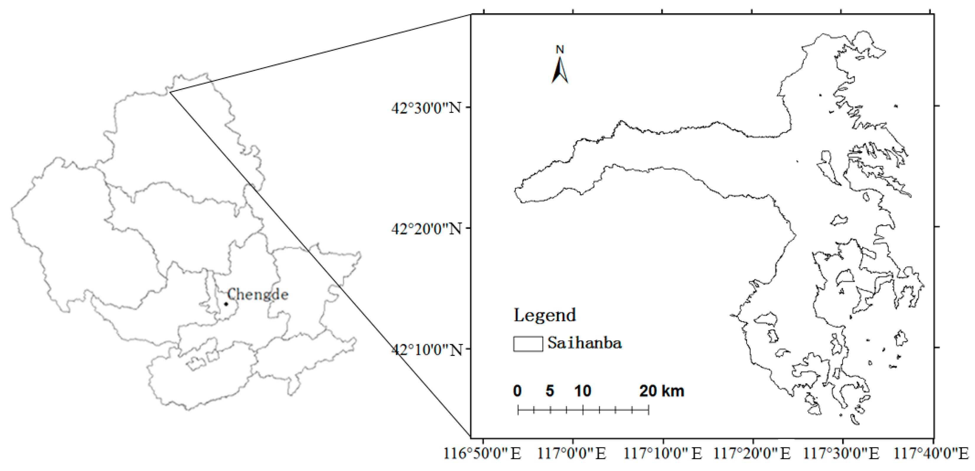
2.1. Study Area

The study area is located in the Saihanba mechanical forestry field, Chengde City, Hebei Province, China, with the latitude and longitude range of 42°04′~42°36′ N and 116°52′~117°39′ E. The study area is 58.6 km long from north to south and 65.5 km wide from east to west, with a total area of about 934.68 km². The area belongs to the southern edge of Inner Mongolia Hunsandak Sandy, where the Inner Mongolia Plateau meets the remainder of the Greater Khingan Mountains and the remainder of the Yinshan Mountains, with an altitude of 1010~1939.9 m. It has a cold-temperate continental monsoon climate, transitioning from semi-humid to semi-arid, with long and cold winters and insignificant summers. It has an extreme maximum temperature of 33.4 °C, minimum temperature of −43.3 °C, average annual temperature of −1.3 °C, average annual frost-free period of about 60 days and average annual precipitation of 490 mm. The forest coverage rate reaches 75.5%, the total forest tree accumulation is 4.62 million m³ and the soil is mainly aeolian sandy soil, meadow soil, brown loam and grey forest soil [67,68]. The area of artificial afforestation is 573.33 km² and natural forest is 160 km². The tree species are mainly northern Chinese larch (Larix principis-ruprechtii), camphor pine (Pinus sylvestris var. mongolica), spruce (Picea asperata) and silver birch (Betula platyphylla). The location of the study area is shown in Figure 1.

2.2. Data and Preprocessing

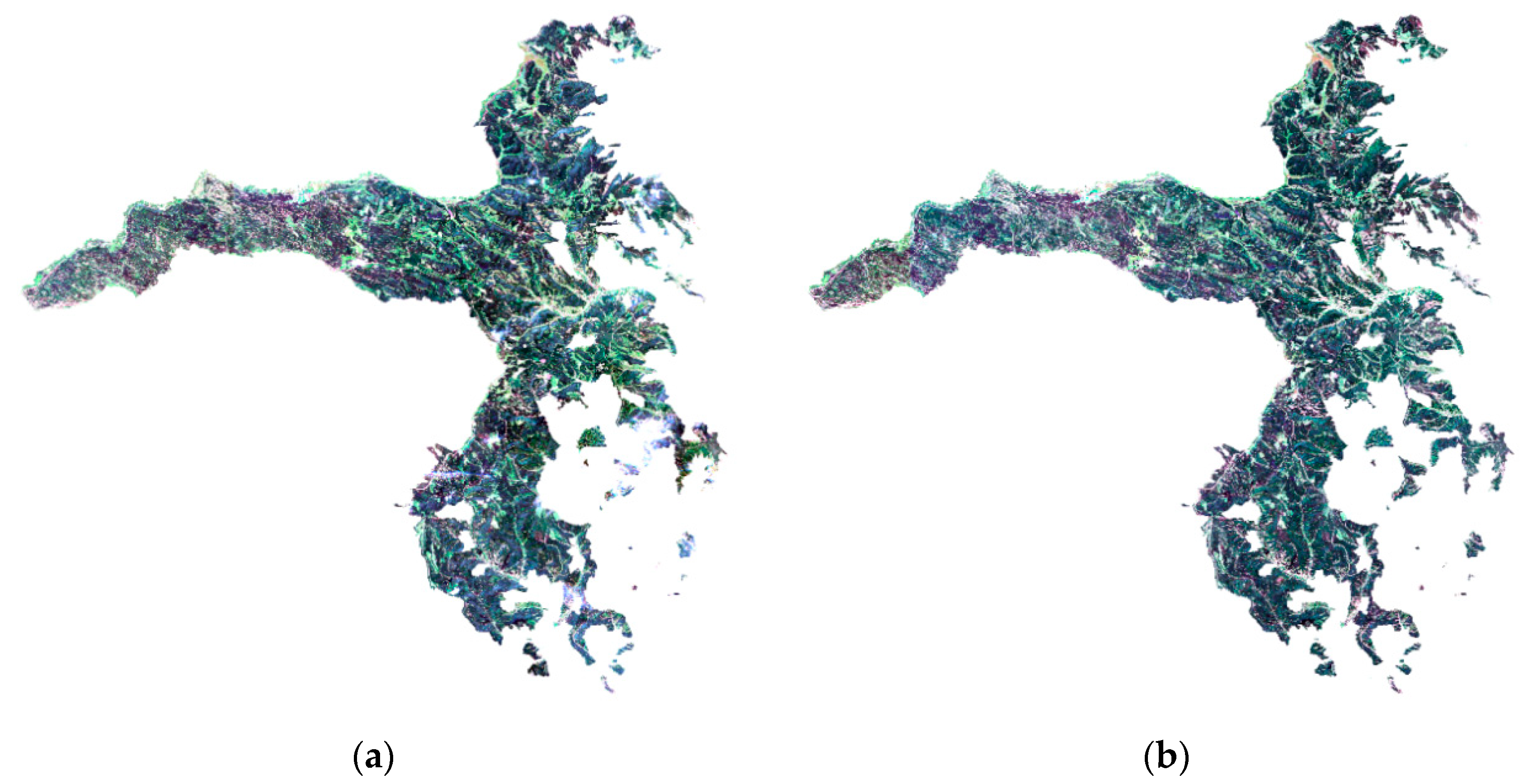
2.2.1. Remote Sensing Data and Pre-Processing

The leaves of the study area were fully expanded around July and August when the leaf area index was considered to have basically reached its maximum value and remained basically constant over a certain period of time. The remote sensing data used for the LAI inversion and estimation of the maximum LAI came from the Sentinel-2 satellite image taken on 21 August 2019, with image level L2A, good image quality and basically cloud-free, and the remote sensing image map of the study area was obtained after clipping, as shown in Figure 2a. At the same time, the Sentinel-2 satellite image on 25 August 2020 was acquired to verify the leaf area estimation model, and the image preprocessing was consistent with that in 2019, as shown in Figure 2b. When extracting VIs from the images, the average value of the pixel at the coordinate center and its surrounding eight pixels was used as the VI of the sample plot.

The MCD15A3H product (orbit number h26v04) for the study area in 2019, including LAI and photosynthetically active radiation, was obtained via the NASA website with a spatial resolution of 500 m and a temporal resolution of 4 days, for a total of 92-time phases of LAI images per year. The MODIS LAI images were pre-processed with image cropping and projection conversion to construct the time-series LAI data for 92 time phases per year in the study area. The LAI time-series curves were extracted from the MODIS LAI raster dataset. In this study, the time-series LAI data were smoothed using the locally adjusted cubic-spline capping (LACC) algorithm proposed by Chen et al. [69]. The smoothed MODIS LAI dataset was used as the base dataset for further study.

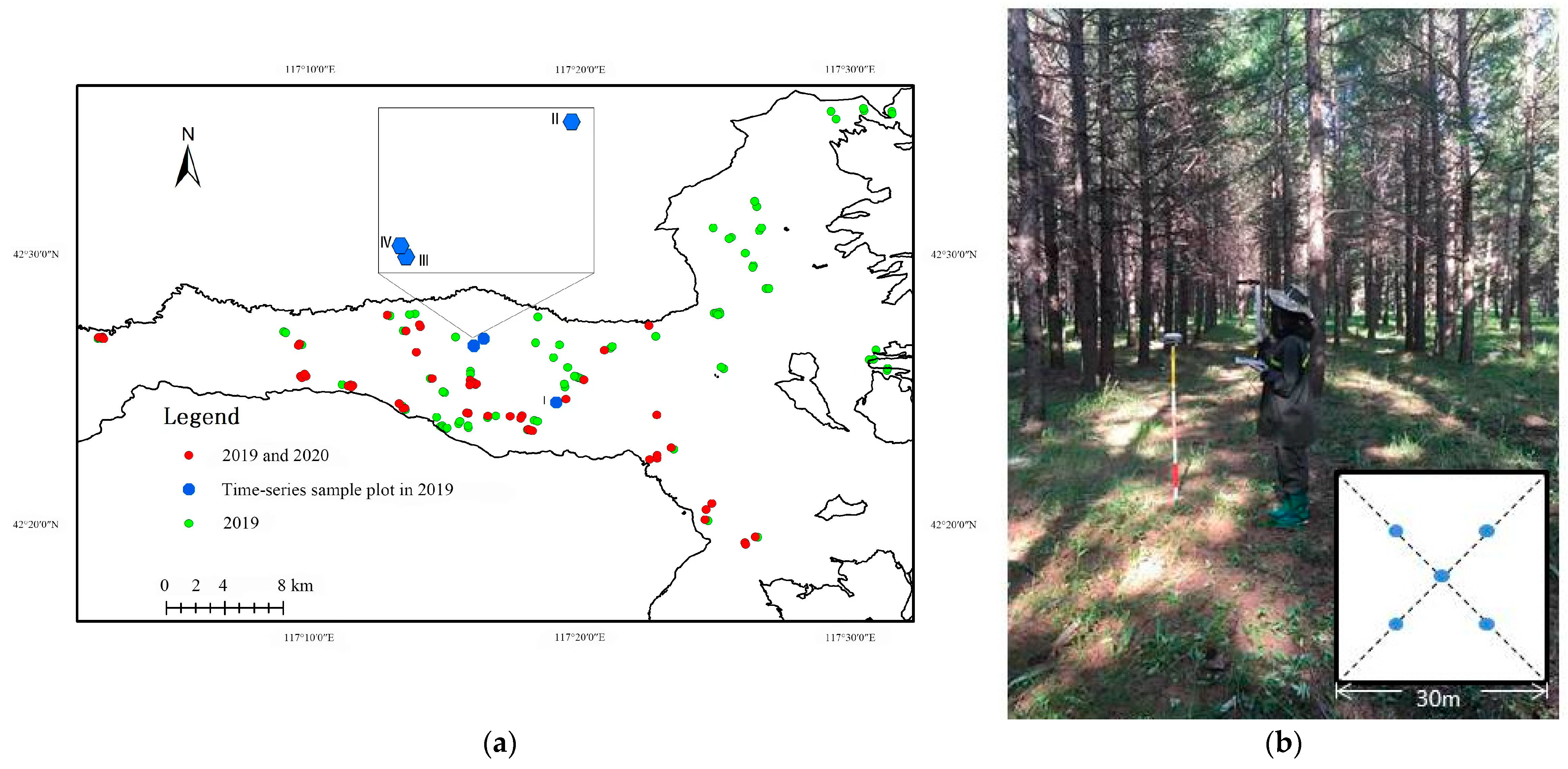
2.2.2. LAI Field Measurements

The LAI observations were collected with the LAI-2200 vegetation canopy analyzer from LI-COR, USA, and the collection was conducted mainly on cloudy days or the collection times were concentrated between 07:00 and 10:00 a.m. and 04:00 and 07:00 p.m. to avoid errors due to direct sunlight. In this study, data were collected between 24 July 2019 and 24 August 2019, and 139 random sample plots of planted coniferous pure forests with a sample plot size of 30 × 30 m were selected for measurement. In order to facilitate accurate matching between the actual measurement points and remote sensing images, real time kinematic (RTK) was used to locate each random sample location in the experiment. Four points were evenly selected for observation at each sample site location and within 10 m of the surrounding area, and five LAI data were obtained and averaged as the observation results of one sample site. Between 10 August 2020 and 22 August 2020, 47 of the 139 samples measured in 2019 were randomly selected for repeated measurement, and the measurement method was consistent with that in 2019.

Field LAI time-series measurements of the study area were conducted in 2019 using LAI-2200, with four sample plots. The size of each sample plot was 30 × 30 m, and the data were collected between May and October, 2019. Field measurements of the sample plots are shown in Figure 3. Coordinates of the time-series LAI sample plots are shown in

Table 2. Coordinates of the Time-series LAI sample plots.

Sample Plot	Coordinates
Ⅰ	117.3185° N, 42.40883° E
Ⅱ	117.2736° N, 42.44807° E
Ⅲ	117.2676° N, 42.44339° E
Ⅳ	117.2674° N, 42.44396° E

.

2.2.3. Forest Type Data

Using the ArcGIS 10 software and the small-group distribution vector data of the study area, we generated stand type raster data based on its stand type and stand age fields as a reference basis for the stand type and stand age.

2.3. Methods

2.3.1. Construction of Remote Sensing Model for LAI

Referring to the previous research results [70,71,72], the NDVI Normalized Difference Vegetation Index (NDVI), Simple Ration Index (SR), Difference Vegetation Index (DVI) and Atmospherically Resistant Vegetation Index (ARVI) were selected as the input parameters of the model. The specific calculation formulae are shown in

Table 3. Expressions for Vegetation Indices.

Vegetation Index	Formulation
NDVI	(NIR − R)/(NIR + R)
SR	NIR/R
DVI	NIR − R
ARVI	(NIR − RB)/(NIR + RB), RB = NIR − γ(B − R)

NIR, R and B are the surface reflectance of band 8, band 4 and band 2 of Sentinel-2 image, respectively, γ is a variable related to aerosol type and properties, with a value of 1.0.

.

In this study, the estimation of the LAI was carried out in the following three ways: (1) constructing linear and nonlinear estimation models using a single vegetation index, i.e., establishing linear, exponential, logarithmic, multiplicative power and quadratic polynomial regression models for each vegetation index, separately, with the LAI; (2) constructing multivariate linear estimation models using multiple vegetation indices; (3) establishing principal component regression analysis models for computational analysis.

To compare the differences in the LAI estimation by the different vegetation indices and different estimation models, the measured LAI values in the study area were divided into 110 training samples and 29 test samples. The vegetation indices were substituted into the regression equation calculated from the training set to obtain the estimated value of $LA{I}_{mod}$, and then the coefficient of determination $R^2$ and root mean square error RMSE of the regression equation were calculated for the calculated result $LA{I}_{mod}$ and its corresponding true value of $LA{I}_{real}$. The degree of correlation of the equation fit is judged according to $R^2$, which has a value of between 0 and 1. If $R^2$ is closer to 1, it indicates that the reference value of the fitted equation is higher. The calculation formula of $R^2$ and RMSE are as follows.

For linear regressions:

$$R^2=1-{{\displaystyle \sum }}_{i=1}^n{\left(LA{I}_{\mathrm{mod}i}-LA{I}_{\mathrm{real}i}\right)}^2/{{\displaystyle \sum }}_{i=1}^n{\left(LA{I}_{\mathrm{real}i}-LA{I}_{\mathrm{realavg}}\right)}^2$$

(1)

For non-linear regressions:

$$R_{adjust}^2=1-(1-R^2)(n-1)/(n-k-1)$$

(2)

$$\mathit{RMSE}=\sqrt{{{\displaystyle \sum }}_{i=1}^n{\left({LAI}_{\mathrm{mod}i}-{LAI}_{\mathrm{real}i}\right)}^2/n}$$

(3)

Here, n is the number of samples, k is the number of independent variables. If $R^2$ is closer to 1 and RMSE is closer to 0, the estimation result of the model is closer to the real value.

2.3.2. Normalized LAI Growth Function and Daily LAI Calculation

LAI(t) represents the growth function of the LAI with time, which is closely related to the stand type, stand age and stand density. LAI(t) of temperate forest is a single peak curve. The normalized LAI growth function ${LAI}_{norm}$(t) is also a single peak, indicating the growth degree or defoliation degree of leaves. The calculation formula is as follows:

$$LA{I}_{norm}\left(t\right)=\left(LAI\left(t\right)-LA{I}_{min}\right)/\left(LA{I}_{max}-LA{I}_{min}\right)$$

(4)

Here, t indicates the number of days in the day sequence. LAI(t) represents the LAI value at time t, i.e., the LAI growth function. ${LAI}_{norm}\left(t\right)$ represents the normalized LAI growth function, which changes with stand age and stand type. ${LAI}_{min}$ is the minimum value of LAI in a year. ${LAI}_{max}$ represents the maximum value of LAI in a year, which occurs after complete leaf spread and changes little in a period of time, during which all LAI measurements can be used as ${LAI}_{max}$.

The object of this study is a cold temperate coniferous forest, and the ${LAI}_{min}$ is approximately 0; then, Equation (4) is simplified to Equation (5), and ${LAI}_{norm}\left(t\right)$ is expressed as the proportional fraction of $LAI\left(t\right)$ and ${LAI}_{max}$.

$${LAI}_{norm}\left(t\right)=LAI\left(t\right)/{LAI}_{max}$$

(5)

$$\mathit{LAI}\left(t\right)={LAI}_{norm}\left(t\right)\times {LAI}_{max}$$

(6)

Due to the difference in stand density, the LAI(t) of every location is different. The LAI(t) obtained in a large area cannot represent the LAI of each internal sub area; that is, the LAI value extracted from the large pixel of the MODIS LAI data cannot represent the LAI value of its internal sub area. However, the ${LAI}_{norm}$(t) of the identical stand type or similar age are basically consistent, and the${LAI}_{norm}$(t) obtained on a larger MODIS raster area with a single stand type or similar age can almost represent the normalized growth of the LAI of each small image within the large image. If the${LAI}_{norm}$(t) and its ${LAI}_{max}$ are obtained for the small image element, the LAI growth curve can be obtained according to Equation (6). The single image element of forest stand types and the normalized LAI growth function can be extracted from MODIS LAI products as the corresponding ${LAI}_{norm}$(t) of the small image element. The spatial resolution of the Sentinel-2 image is 10 m, which is a more suitable data source for extracting the ${LAI}_{max}$ on the scale of small and medium areas. ${LAI}_{max}$ distribution maps can be obtained according to the traditional LAI remote sensing inversion model and the Sentinel-2 image obtained at the complete vegetation spreading leaf period, and the 10 m resolution LAI distribution maps can reflect the spatial heterogeneity of the LAI in small and medium-sized regions.

3. Results

3.1. Remote Sensing Model of LAI in Saihanba Area

3.1.1. Univariate Regression Analysis

Establish the single factor linear regression model and quadratic, logarithm, power, exponential and other nonlinear regression models with four vegetation indexes and LAI, respectively, and calculate $R^2$ and RMSE. The results are shown in

Table 4. Comparison of Unitary Regression Models.

VI	Equation Type	Regression Equation	${\mathit{R}}^2$	RMSE
NDVI	Linear	LAI = 12.786NDVI − 7.48	0.392	0.457
	Quadratic	LAI$=-24.742NDV{I}^2$ + 53.13NDVI − 23.933	0.393	0.454
	Logarithm	LAI = 10.422In NDVI + 4.093	0.393	0.454
	Power	LAI$=6.243NDV{I}^{3.804}$	0.423	0.443
	Exponential	LAI = 0.071exp(4.662NDVI)	0.42	0.444
	Linear	LAI = 0.198SR + 0.964	0.374	0.463
	Quadratic	LAI$=-0.012S{R}^2+0$.448SR − 0.356	0.381	0.459
SR	Logarithm	LAI = 2.068In SR + 0.865	0.385	0.457
	Power	LAI$=0.493S{R}^{0.749}$	0.401	0.451
	Exponential	LAI = 1.438exp(0.066SR)	0.375	0.461
	Linear	LAI = 0.001DVI + 0.825	0.198	0.525
	Quadratic	LAI$=-2.384\times {10}^{-7}DV{I}^2$ $+0$.002DVI + 0.151	0.208	0.519
DVI	Logarithm	LAI = 1.375In DVI − 1.48	0.207	0.519
	Power	LAI$=0.088DV{I}^{0.459}$	0.186	0.526
	Exponential	LAI = 1.953exp(0.002DVI)	0.178	0.529
	Linear	LAI = 10.729ARVI − 5.992	0.429	0.443
	Quadratic	LAI$=-2.229ARV{I}^2+1$4.381ARVI − 7.479	0.43	0.44
ARVI	Logarithm	LAI = 8.777In ARVI + 4.509	0.429	0.441
	Power	LAI$=5.258ARV{I}^{3.317}$	0.499	0.413
	Exponential	LAI = 0.102exp(4.043ARVI)	0.493	0.415

.

From the results of the linear and nonlinear regression models of the LAI and single vegetation index, the optimal regression equation of the DVI is a quadratic equation, and the respective optimal regression equations of the NDVI, SR and ARVI are power equations. The regression models of the NDVI and SR are not as effective as the ARVI, the estimation effect of the power regression equation of the ARVI and LAI was the best ($R^2$ = 0.499, RMSE = 0.413), while the regression model of the DVI and LAI was relatively worse than that of the other three single factor regression models of the vegetation index.

3.1.2. Multiple Linear Regression Analysis

Four vegetation indices were selected to study the multivariate linear statistical model with different combinations, and the $R^2$ and RMSE were calculated to find the best combination of vegetation indices; the results are shown in

Table 5. Comparison of Multiple Regression Models.

VIs Combinations	Regression Equation	${\mathit{R}}^2$	RMSE
NDVI, SR	LAI = 13.716NDVI − 0.014SR − 8.075	0.519	0.403
NDVI, DVI	LAI = 13.688NDVI − 0.000074DVI − 8.056	0.521	0.402
NDVI, ARVI	LAI = 11.228ARVI − 0.664NDVI − 5.859	0.528	0.399
SR, DVI	LAI = 0.221SR + 0.00001DVI + 0.544	0.512	0.406
SR, ARVI	LAI = 0.026SR + 9.435ARVI − 5.188	0.531	0.398
DVI, ARVI	LAI = 10.175ARVI + 0.000069DVI − 5.672	0.532	0.397
NDVI, SR, DVI	LAI = 12.058NDVI + 0.03SR − 0.000097DVI − 6.981	0.533	0.395
NDVI, SR, ARVI	LAI = 15.109ARVI + 0.205SR − 18.42NDVI + 3.268	0.545	0.39
SR, DVI, ARVI	LAI = 9.832ARVI + 0.000052DVI + 0.011SR − 5.461	0.533	0.395
NDVI, DVI, ARVI	LAI = −4.713NDVI + 13.201ARVI + 0.00019DVI − 4.496	0.539	0.392
NDVI, SR, DVI, ARVI	LAI = −18.322NDVI + 0.192SR + 0.000043DVI + 15.445ARVI + 2.95	0.561	0.381

.

As shown in Table 5, among the equations of the two vegetation indices, the best effect is the DVI and ARVI ($R^2$ = 0.532, RMSE = 0.397). Among the equations of the three vegetation indices, the best effect is the NDVI, SR, ARVI ($R^2$ = 0.545, RMSE = 0.39). The regression equation fitting effect of the four VIs is better than the two VIs and the three VIs ($R^2$ = 0.561, RMSE = 0.381).

3.1.3. PCA Model

Using the PCA method, the principal components were extracted for coniferous forests, and the contribution of each principal component was analyzed (

Table 6. Contribution rate of PCA component.

Principal Component	Characteristic Value	Variance Contribution/%	Cumulative Contribution/%
${\mathit{C}}_1$	3.523	88.075	88.075
${\mathit{C}}_2$	0.411	10.275	98.35
${\mathit{C}}_3$	0.057	1.425	99.775
${\mathit{C}}_4$	0.009	0.225	100.000

), leading to the development of a principal component regression model for LAI estimation based on each vegetation index. The components in the table are the principal components $C_i$ (i = 1, 2, 3, 4) derived by conducting PCA.

As can be seen from Table 6, the cumulative contribution of the first two principal components was 98.35%, which can retain as much information about the original variables as possible. Accordingly, the principal component regression model of the vegetation index and LAI is shown in Equation (7), with $R^2$= 0.554 and RMSE = 0.384.

LAI = 3.592NDVI + 0.033SR − 0.00032DVI + 4.687ARVI − 3.553

(7)

As seen above, the $R^2$ of the principal component regression model for coniferous forests decreased instead. Therefore, the multiple regression model of four VIs was used in the prediction of the LAI of coniferous forests in the study area.

Using the above results to estimate the LAI of the study area on 21 August 2019, the distribution is shown in Figure 4a, and using 29 validation data for accuracy verification, the $R^2$ of the regression equation between the estimated LAI and the measured LAI was 0.85 (Figure 4c), which can be used as a source of ${\mathrm{LAI}}_{\max }$ data. At the same time, the LAI of the study area on 25 August 2020 was estimated. The distribution is shown in Figure 4b. Overall, 47 validation data were used for accuracy verification. The $R^2$ of the regression equation between the estimated LAI and the measured LAI was 0.72 (Figure 4d).

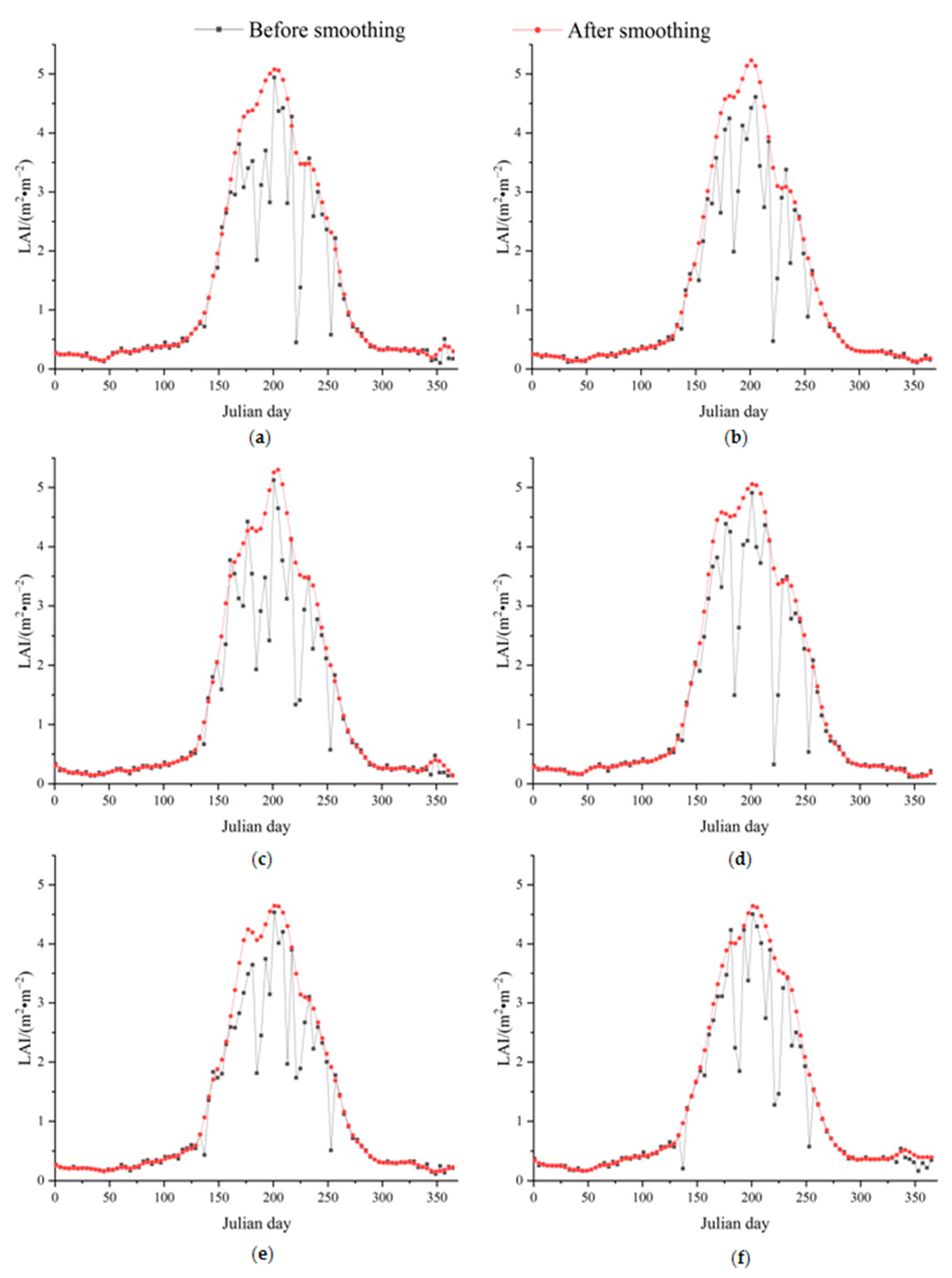
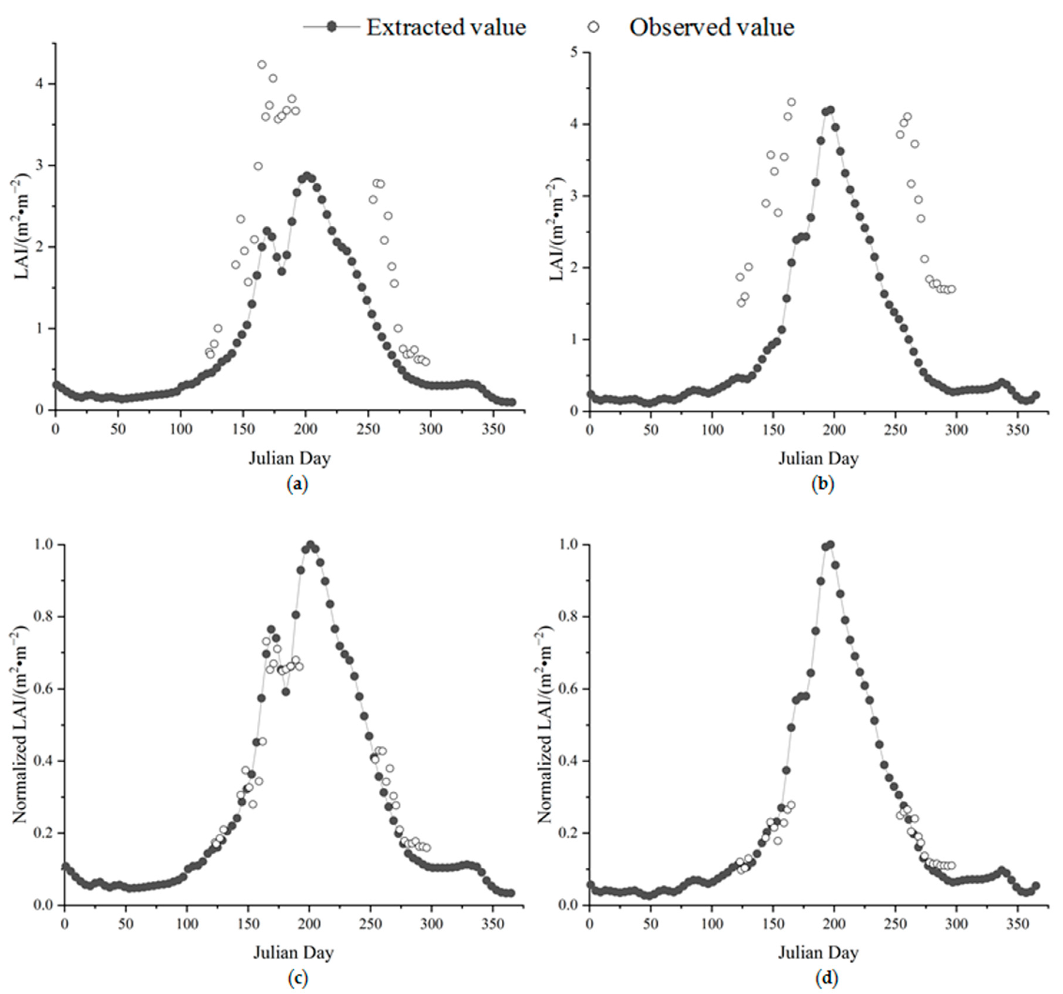
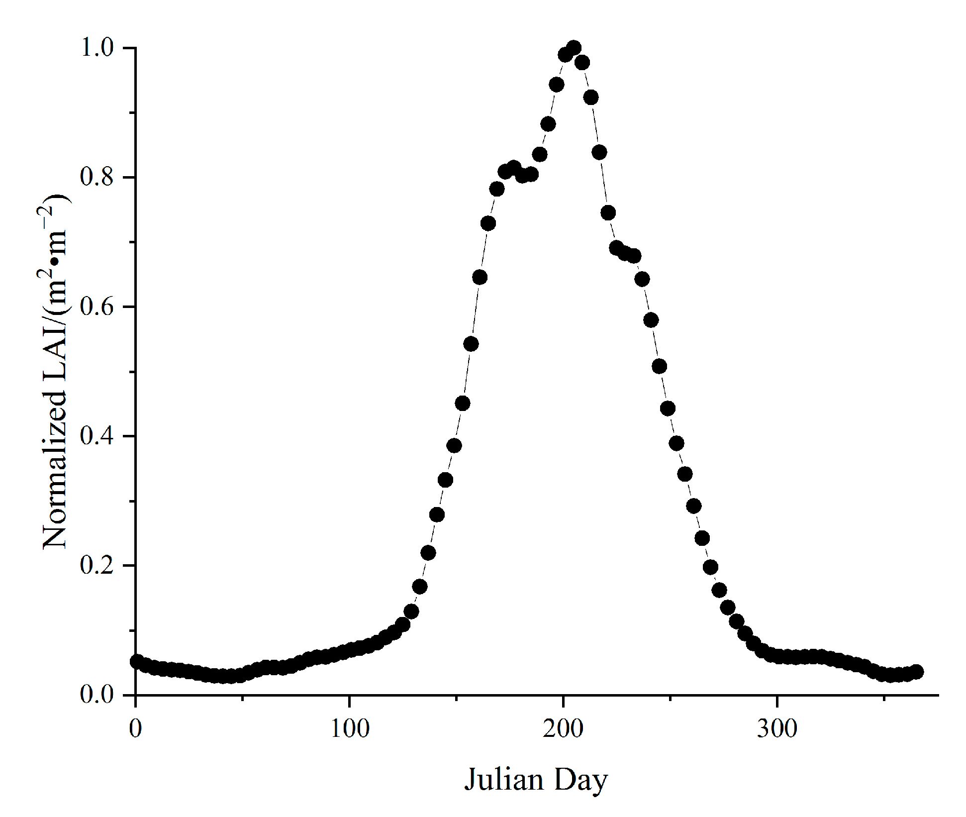
3.2. MODIS LAI Normalized Growth Curve Extraction

The comparison of the LAI curves before and after smoothing is shown in Figure 5. It can be seen that the LAI time-series curves showed uneven seasonal variations. There is little difference between the LAI growth curves extracted from MODIS for age group 0 to age group 5 of coniferous forests in the study area.

From Figure 6, there is a visible difference between the LAI growth curves extracted from MODIS and the measured LAI values. One of the main reasons for this difference was the scale mismatch between the estimated value and the measured value. Despite this difference, the MODIS-extracted LAI curves remained consistent with the growth trend of the actual LAI. In order to better illustrate this problem, this study normalized the MODIS LAI growth curves and the actual LAI values. As can be seen in Figure 6, the normalized MODIS LAI growth curves are in good agreement with the normalized measured LAI values.

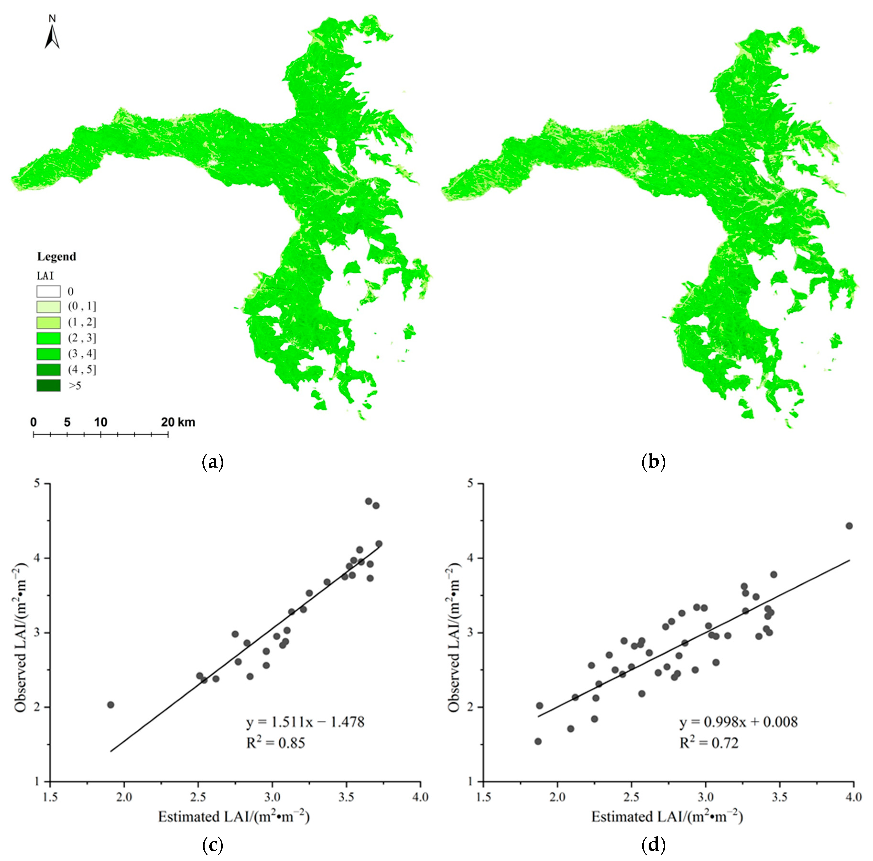
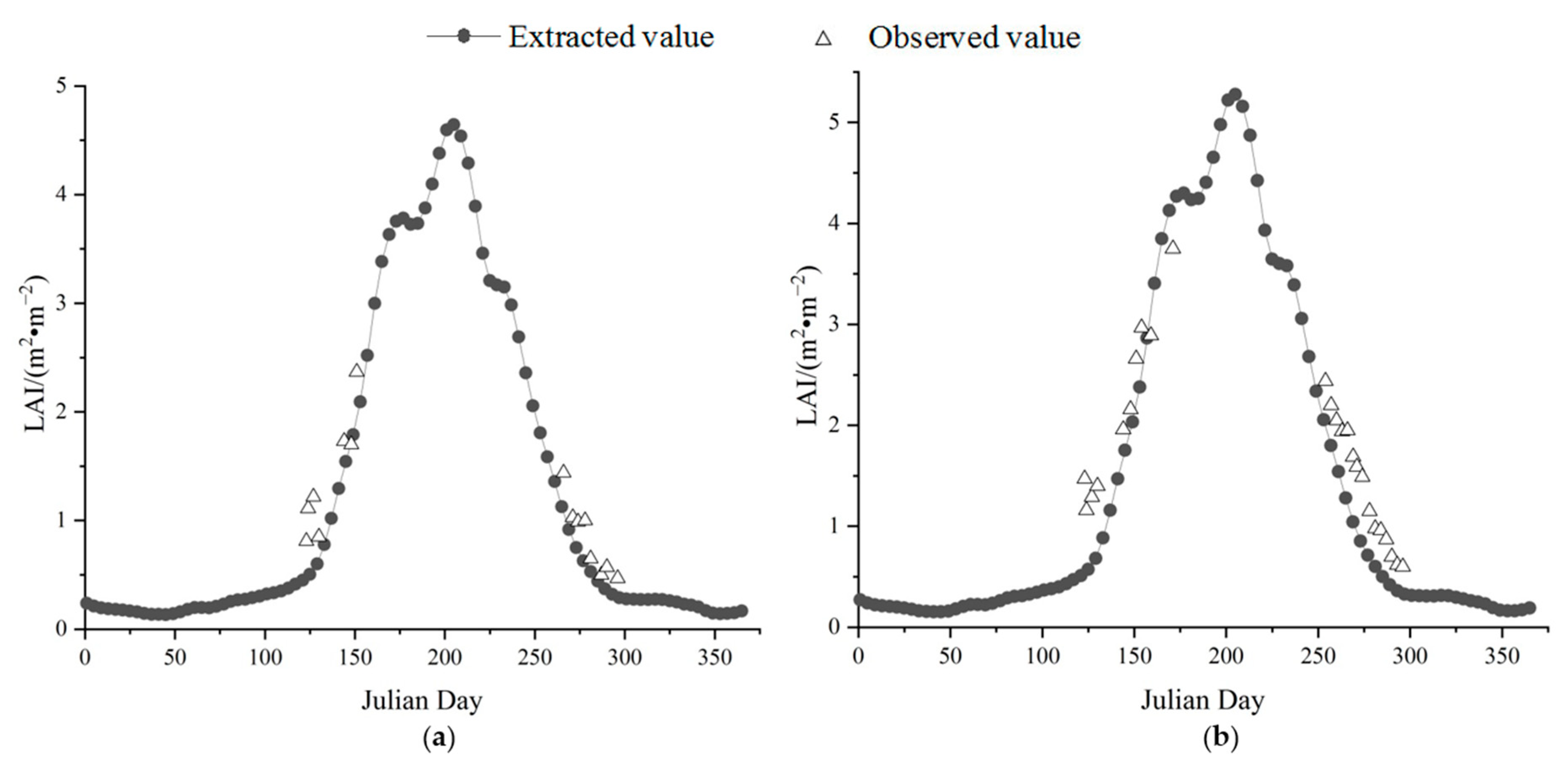
3.3. Daily LAI Calculation of Small and Medium-Sized Regional Scale

When calculating the daily LAI, the LAI normalized growth curve was required. In order to make the LAI normalized curve more representative of the average LAI growth condition of the forest stands in the study area, the vector map of the small group distribution in the study area was overlaid with the smoothed MODIS LAI dataset, and the pure forest region of interest (ROI) points of coniferous forests were selected evenly in the study area. In order to avoid the heterogeneity of the MODIS pixels covering the surface and including the spatial change information of the heterogeneous surface, pure pixels of the stand type should be selected as much as possible to minimize the estimation error of the Sentinel-2 LAI temporal and spatial distribution caused by MODIS mixed pixels, and the extracted normalized LAI should be averaged, as shown in Figure 7. Based on Equation (6), the daily LAI calculation was realized.

The time-series LAI data of two measured points were extracted from the daily LAI data set of the simulated study area and compared with the measured values (Figure 8). It can be seen that compared with the LAI growth curve directly extracted from MODIS in Figure 6, the LAI growth curve obtained using this method matched better with the measured LAI of the sample plot, with RMSE = 0.266 for sample plot Ⅲ and RMSE = 0.478 for sample plot IV.

4. Discussion

As the commonly used remote sensing data cannot meet the high spatial and temporal resolution simultaneously, some researchers [51,53,73] have tried to obtain the high spatial and temporal resolution data by fusing the high spatial resolution data and the high temporal resolution data using the spatial and temporal data fusion model. However, there are still large difficulties and uncertainties in spatio-temporal data fusion during summer in cloudy and rainy areas. Ovakoglou et al. [74] developed a methodology for downscaling the coarse spatial resolution of MODIS LAI images to a higher resolution, and the results showed moderate to high correlation for most cases, while lower accuracies were observed during the rainy season for all the study areas. Data fusion with high temporal and spatial resolution has been successfully applied to crop growth monitoring in previous research [64,66]. However, it has rarely been applied in forest growth factor retrieval. For the Sentinel-2 data fused with the MODIS LAI data at a 4-day interval, this study proposes a fast forest land LAI reconstruction method at small and medium regional scales to reconstruct the LAI images of the Saihanba area.

Sentinel-2 data have a spatial resolution of up to 10 m, which is higher than the Landsat series in all similar bands; therefore, it is helpful for producing higher spatio-temporal fusion image accuracy. The accuracy of Sentinel-2 data depends on its image level and processing level. Kganyago et al. [75] proposed that there are marked differences between the processing levels and insignificant differences between the spatial resolutions of the SNAP-derived LAI. The analysis results in this study show that the multiplicative power regression model of the ARVI has proper inversion accuracy for the forested LAI in Saihanba.

In this study, MODIS LAI data with a 4-day interval were used as the input data for the normalized LAI curves of forest land. The unsmoothed MODIS LAI curves showed large fluctuations, up and down, in the curves due to cloud and shadow images, but still showed the year-round variation trend. After LACC smoothing, the stand LAI curves conform to the year-round variation of tree leaves. By grouping the stand ages, it can be found that the year-round change trend of the stand LAI curve is almost the same between different stand ages. Therefore, this study concluded that the annual change trend in the LAI is not related to the age of the stand.

The annual LAI extracted from the MODIS LAI was compared with the field observation, and the two were found to be in poor numerical agreement. After normalizing the two curves separately, the trends of the normalized curves were in good agreement. This indicates that the MODIS LAI normalized curves can better reflect the annual change of the forest land LAI.

In this study, while the results are promising, there are several opportunities for enhancing the model further. First, the LAI dataset smoothed using the LACC algorithm for MODIS LAI products fluctuated slightly during the leaf spreading period. It was speculated that the reason for this was cloud interference. How to remove the cloud accurately needs further research and improvement. Second, based on the current study, results would be achieved if the measurements of the LAI as $LA{I}_{max}$ and the LAI annual curve are carried out jointly. Third, broad leaved forest needs to be considered to improve this model in the future.

5. Conclusions

Saihanba Machinery Forest Farm is the largest artificial forest farm in the world. The LAI is an important parameter to describe vegetation growth. Therefore, the acquisition of the LAI of forest land in a continuous time-series is very important for the statistics of the carbon storage and carbon sink of forest farms. In order to quickly obtain the forest land LAI data with high spatial and temporal resolution, this study proposes a reconstruction method based on Sentinel-2 data and MODIS LAI data. This study analyzes the accuracy of the LAI data of the reconstructed time-series forest land.

The LAI curves of young, medium, near, adult and past forest ages of the coniferous forest in the study area extracted from the MODIS LAI products had little difference, indicating that the coniferous forest in the study area can use one curve to fit the annual changes.

The remote sensing statistical estimation model of the LAI was developed using the atmospherically resistant vegetation index (ARVI), and the $R^2$ between the estimated LAI and the measured LAI was 0.494.

The regional daily LAI estimation method proposed in this study used MODIS LAI products to extract the LAI normalized growth curve and the traditional remote sensing statistical model to estimate the maximum LAI. The method of simply multiplying them to estimate the time-series LAI was applicable to small- and medium-sized regional scales. Compared with the measured values, the RMSE of sample Ⅲ was 0.268 and the RMSE of sample IV was 0.48. This method was simple and fast in providing effective and high-resolution time-series LAI data for other studies at small and medium regional scales.

This study shows that the combination of high spatial resolution (Sentinel-2 data) and high temporal resolution (MODIS LAI data) can accurately reconstruct the forest land time-series LAI in the study area. The method in this study can be used to reconstruct the LAI of time-series forest land with larch forests of different ages in cloudy areas. Therefore, it is of great significance to accurately count carbon stocks and sinks on a small- and medium-sized regional scale.

References

1. Mao, Y.; Michel, O.; Yu, Y.; Fan, W.; Sui, A.; Liu, Z.; Wu, G. Retrieval of Boreal Forest Heights Using an Improved Random Volume over Ground (RVoG) Model Based on Repeat-Pass Spaceborne Polarimetric SAR Interferometry: The Case Study of Saihanba, China. Remote Sens. 2021, 13, 4306. [Google Scholar] [CrossRef]
2. Owe, M.; Tian, Q.; D’Urso, G.; Chen, J.M.; Zheng, G.; Neale, C.M.U.; Gouweleeuw, B.T.; Xia, X.; Chen, J. Quantitative retrieving forest ecological parameters based on remote sensing in Liping County of China. Remote Sens. Agric. Ecosyst. Hydrol. VIII 2006, 6539, 317–326. [Google Scholar] [CrossRef]
3. Hall, F.G.; Bergen, K.; Blair, J.B.; Dubayah, R.; Houghton, R.; Hurtt, G.; Kellndorfer, J.; Lefsky, M.; Ranson, J.; Saatchi, S.; et al. Characterizing 3D vegetation structure from space: Mission requirements. Remote Sens. Environ. 2011, 115, 2753–2775. [Google Scholar] [CrossRef] [Green Version]
4. Yang, L.; Robert, T.; Fabio, G. Automated estimation of forest height and underlying topography over a Brazilian tropical forest with single-baseline single-polarization TanDEM-X SAR interferometry. Remote Sens. Environ. 2021, 252, 112132. [Google Scholar] [CrossRef]
5. Houghton, R.A.; Hall, F.; Goetz, S.J. Importance of biomass in the global carbon cycle. J. Geophys. Res. Biogeosci. 2009, 114, G00E03. [Google Scholar] [CrossRef]
6. Myneni, R.B.; Hoffman, S.; Knyazikhin, Y.; Privette, J.L.; Glassy, J. Global products of vegetation leaf area and fraction absorbed par from year one of modis data. Remote Sens. Environ. 2002, 83, 214–231. [Google Scholar] [CrossRef] [Green Version]
7. Gao, W.; Walthall, C.L.; Shaw, D.R.; Dulaney, W.P.; Anderson, M.C.; Norman, J.; Fang, H.; Liang, S.; Timlin, D.J.; Pachepsky, Y. Alternative approaches for estimating leaf area index (LAI) from remotely sensed satellite and aircraft imagery. Remote Sens. Model. Ecosyst. Sustain. 2004, 5544, 241–255. [Google Scholar] [CrossRef]
8. Arora, V. Modeling Vegetation as a Dynamic Component in Soil-Vegetation-Atmosphere Transfer Schemes and Hydrological Models. Rev. Geophys. 2002, 40, 3-1–3-26. [Google Scholar] [CrossRef] [Green Version]
9. Sellers, P.J. Modeling the Exchanges of Energy, Water, and Carbon Between Continents and the Atmosphere. Science 1997, 275, 502–509. [Google Scholar] [CrossRef] [Green Version]
10. Ge, J. On the Proper Use of Satellite-Derived Leaf Area Index in Climate Modeling. J. Clim. 2009, 22, 4427–4433. [Google Scholar] [CrossRef]
11. Luo, S.; Wang, C.; Zhang, G.; Xi, X.; Li, G. Forest Leaf Area Index (LAI) Estimation Using Airborne Discrete-Return Lidar Data. Chin. J. Geophys. 2013, 56, 233–242. [Google Scholar] [CrossRef]
12. Sellers, P.J.; Mintz, Y.; Sud, Y.C.; Dalcher, A. A Simple Biosphere Model (SIB) for Use within General Circulation Models. J. Atmos. Sci. 1986, 43, 505–531. [Google Scholar] [CrossRef]
13. Xu, J.; Quackenbush, L.J.; Volk, T.A.; Im, J. Forest and Crop Leaf Area Index Estimation Using Remote Sensing: Research Trends and Future Directions. Remote Sens. 2020, 12, 2934. [Google Scholar] [CrossRef]
14. Muhammad, A.; Carsten, M.; Anja, S.; Gunter, M.; Frank, T.; Harry, V. Estimation and Validation of RapidEye-Based Time-Series of Leaf Area Index for Winter Wheat in the Rur Catchment (Germany). Remote Sens. 2015, 7, 2808–2831. [Google Scholar] [CrossRef] [Green Version]
15. Quan, X.; He, B.; Wang, Y.; Tang, Z.; Li, X. An Extended Fourier Approach to Improve the Retrieved Leaf Area Index (LAI) in a Time Series from an Alpine Wetland. Remote Sens. 2014, 6, 1171–1190. [Google Scholar] [CrossRef] [Green Version]
16. Myneni, R.B.; Ramakrishna, R.; Nemani, R.; Running, S.W. Estimation of global leaf area index and absorbed par using radiative transfer models. IEEE Trans. Geosci. Remote Sens. 1997, 35, 1380–1393. [Google Scholar] [CrossRef] [Green Version]
17. Houborg, R.; Anderson, M.C. Utility of an image-based canopy reflectance modeling tool for remote estimation of LAI and leaf chlorophyll content at regional scales. J. Appl. Remote Sens. 2009, 3, 033529. [Google Scholar] [CrossRef]
18. Chen, J.; Pavlic, G.; Brown, L.; Cihlar, J.; Leblanc, S.G. Derivation and validation of canada-wide coarse-resolution leaf area index maps using high-resolution satellite imagery and ground measurements. Remote Sens. Environ. 2002, 80, 165–184. [Google Scholar] [CrossRef]
19. Jacquemoud, S.; Verhoef, W.; Baret, F.; Bacour, C.; Zarco-Tejada, P.J.; Asner, G.P.; François, C.; Ustin, S.L. PROSPECT+SAIL models: A review of use for vegetation characterization. Remote Sens. Environ. 2009, 113, S56–S66. [Google Scholar] [CrossRef]
20. Haboudane, D. Hyperspectral vegetation indices and novel algorithms for predicting green LAI of crop canopies: Modeling and validation in the context of precision agriculture. Remote Sens. Environ. 2004, 90, 337–352. [Google Scholar] [CrossRef]
21. Cohen, W.B.; Maiersperger, T.K.; Gower, S.T.; Turner, D.P. An improved strategy for regression of biophysical variables and Landsat ETM+ data. Remote Sens. Environ. 2003, 84, 561–571. [Google Scholar] [CrossRef] [Green Version]
22. Colombo, R. Retrieval of leaf area index in different vegetation types using high resolution satellite data. Remote Sens. Environ. 2003, 86, 120–131. [Google Scholar] [CrossRef]
23. Yotov, K.; Li, X.; Ren, G.; Cibulskis, M.; Dejong, G.; Garzaran, M. A comparison of empirical and model-driven optimization. ACM SIGPLAN Not. 2003, 38, 63–76. [Google Scholar] [CrossRef] [Green Version]
24. Feng, D.; Chen, J.M.; Plummer, S.; Chen, M.; Pisek, J. Algorithm for global leaf area index retrieval using satellite imagery. IEEE Trans. Geosci. Remote Sens. 2006, 44, 2219–2229. [Google Scholar] [CrossRef] [Green Version]
25. Wiegand, C.L.; Maas, S.J.; Aase, J.K.; Hatfield, J.L.; Pinter, P.J.; Jackson, R.D. Multisite analyses of spectral-biophysical data for wheat. Remote Sens. Environ. 1992, 42, 1–21. [Google Scholar] [CrossRef]
26. Stagakis, S.; Markos, N.; Sykioti, O.; Kyparissis, A. Monitoring canopy biophysical and biochemical parameters in ecosystem scale using satellite hyperspectral imagery: An application on a Phlomis fruticosa Mediterranean ecosystem using multiangular CHRIS/PROBA observations. Remote Sens. Environ. 2010, 114, 977–994. [Google Scholar] [CrossRef]
27. Liu, J.; Pattey, E.; Jégo, G. Assessment of vegetation indices for regional crop green LAI estimation from Landsat images over multiple growing seasons. Remote Sens. Environ. 2012, 123, 347–358. [Google Scholar] [CrossRef]
28. Curran, P.J.; Steven, M. Multispectral Remote Sensing for the Estimation of Green Leaf Area Index [and Discussion]. Philos. Trans. R. Soc. A Math. Phys. Eng. Sci. 1983, 309, 257–270. [Google Scholar]
29. Xiao, Z.; Liang, S.; Wang, J.; Xiang, Y.; Zhao, X.; Song, J. Long-Time-Series Global Land Surface Satellite Leaf Area Index Product Derived From MODIS and AVHRR Surface Reflectance. IEEE Trans. Geosci. Remote Sens. 2016, 54, 1–18. [Google Scholar] [CrossRef]
30. Fang, H.; Baret, F.; Plummer, S.; Schaepman-Strub, G. An Overview of Global Leaf Area Index (LAI): Methods, Products, Validation, and Applications. Rev. Geophys. 2019, 57, 739–799. [Google Scholar] [CrossRef]
31. Chen, J.; Jönsson, P.; Tamura, M.; Gu, Z.; Matsushita, B.; Eklundh, L. A simple method for reconstructing a high-quality NDVI time-series data set based on the Savitzky–Golay filter. Remote Sens. Environ. 2004, 91, 332–344. [Google Scholar] [CrossRef]
32. Xiao, Z.; Liang, S.; Wang, J.; Song, J.; Wu, X. A Temporally Integrated Inversion Method for Estimating Leaf Area Index From MODIS Data. IEEE Trans. Geosci. Remote Sens. 2009, 47, 2536–2545. [Google Scholar] [CrossRef]
33. Xie, Y.; Wang, P.; Bai, X.; Khan, J.; Zhang, S.; Li, L.; Wang, L. Assimilation of the leaf area index and vegetation temperature condition index for winter wheat yield estimation using Landsat imagery and the CERES-Wheat model. Agric. For. Meteorol. 2017, 246, 194–206. [Google Scholar] [CrossRef]
34. Chen, Y.; Li, D.; Han, Q.; Zhang, X.; Zhang, Q. Time series assessment of multi-source spatiotemporal fusion reconstruction data based on dynamic time warping. In Proceedings of the IEEE International Conference on Artificial Intelligence and Computer Applications (ICAICA), Dalian, China, 27–29 June 2020; pp. 858–864. [Google Scholar] [CrossRef]
35. Xiao, Z.; Liang, S.; Wang, J.; Wang, Z. Retrieval of Leaf Area Index by Coupling Radiative Transfer Model and a Dynamic Model. In Proceedings of the IEEE International Geoscience and Remote Sensing Symposium, Boston, MA, USA, 6–11 July 2008; pp. v554–v557. [Google Scholar] [CrossRef]
36. Verger, A.; Filella, I.; Baret, F.; Peñuelas, J. Vegetation baseline phenology from kilometric global LAI satellite products. Remote Sens. Environ. 2016, 178, 1–14. [Google Scholar] [CrossRef] [Green Version]
37. Xun, L.; Wang, P.; Li, L.; Wang, L.; Kong, Q. Identifying crop planting areas using Fourier-transformed feature of time series MODIS leaf area index and sparse-representation-based classification in the North China Plain. Int. J. Remote Sens. 2018, 40, 2034–2052. [Google Scholar] [CrossRef]
38. Feng, G.; Martha, C.A.; William, P.K.; Wang, Y.J. Simple method for retrieving leaf area index from Landsat using MODIS leaf area index products as reference. J. Appl. Remote Sens. 2012, 6, 063554. [Google Scholar] [CrossRef]
39. Propastin, P.; Panferov, O. Retrieval of remotely sensed LAI using Landsat ETM+ data and ground measurements of solar radiation and vegetation structure: Implication of leaf inclination angle. Int. J. Appl. Earth Obs. Geoinf. 2013, 25, 38–46. [Google Scholar] [CrossRef]
40. Turner, D.P.; Cohen, W.B.; Kennedy, R.E.; Fassnacht, K.S.; Briggs, J.M. Relationships between Leaf Area Index and Landsat TM Spectral Vegetation Indices across Three Temperate Zone Sites. Remote Sens. Environ. 1999, 70, 52–68. [Google Scholar] [CrossRef]
41. Schlerf, M.; Atzberger, C. Inversion of a forest reflectance model to estimate structural canopy variables from hyperspectral remote sensing data. Remote Sens. Environ. 2006, 100, 281–294. [Google Scholar] [CrossRef]
42. Knyazikhin, Y.; Martonchik, J.V.; Myneni, R.B.; Diner, D.J.; Running, S.W. Synergistic algorithm for estimating vegetation canopy leaf area index and fraction of absorbed photosynthetically active radiation from MODIS and MISR data. J. Geophys. Res. Atmos. 1998, 103, 32257–32275. [Google Scholar] [CrossRef] [Green Version]
43. Zhu, Z.; Bi, J.; Pan, Y.; Ganguly, S.; Anav, A.; Xu, L.; Samanta, A.; Piao, S.; Nemani, R.; Myneni, R. Global Data Sets of Vegetation Leaf Area Index (LAI)3g and Fraction of Photosynthetically Active Radiation (FPAR)3g Derived from Global Inventory Modeling and Mapping Studies (GIMMS) Normalized Difference Vegetation Index (NDVI3g) for the Period 1981 to 2011. Remote Sens. 2013, 5, 927–948. [Google Scholar] [CrossRef] [Green Version]
44. Baret, F.; Weiss, M.; Lacaze, R.; Camacho, F.; Makhmara, H.; Pacholcyzk, P.; Smets, B. GEOV1: LAI and FAPAR essential climate variables and FCOVER global time series capitalizing over existing products. Part1: Principles of development and production. Remote Sens. Environ. 2013, 137, 299–309. [Google Scholar] [CrossRef]
45. Zhang, W.; Li, A.; Jin, H.; Bian, J.; Zhang, Z.; Lei, G.; Qin, Z.; Huang, C. An Enhanced Spatial and Temporal Data Fusion Model for Fusing Landsat and MODIS Surface Reflectance to Generate High Temporal Landsat-Like Data. Remote Sens. 2013, 5, 5346–5368. [Google Scholar] [CrossRef] [Green Version]
46. Hilker, T.; Wulder, M.A.; Coops, N.C.; Linke, J.; McDermid, G.; Masek, J.G.; Gao, F.; White, J.C. A new data fusion model for high spatial- and temporal-resolution mapping of forest disturbance based on Landsat and MODIS. Remote Sens. Environ. 2009, 113, 1613–1627. [Google Scholar] [CrossRef]
47. Lu, W.; Fan, W. Fast estimation method for time-series forest LAI at small and medium regional scale. Trans. Chin. Soc. Agric. Eng. (Trans. CSAE) 2016, 32, 188–193. [Google Scholar] [CrossRef]
48. Zhu, X.; Cai, F.; Tian, J.; Williams, T. Spatiotemporal Fusion of Multisource Remote Sensing Data: Literature Survey, Taxonomy, Principles, Applications, and Future Directions. Remote Sens. 2018, 10, 527. [Google Scholar] [CrossRef] [Green Version]
49. Cai, Z.; Junttila, S.; Holst, J.; Jin, H.; Ard, J.; Ibrom, A.; Peichl, M.; Mölder, M.; Jönsson, P.; Rinne, J.; et al. Modelling Daily Gross Primary Productivity with Sentinel-2 Data in the Nordic Region–Comparison with Data from MODIS. Remote Sens. 2021, 13, 469. [Google Scholar] [CrossRef]
50. Georgia, D.; Zina, M.; Ferran, G.; Philippe, G.; Bojan, B. A Spectral Unmixing Model for the Integration of Multi-Sensor Imagery: A Tool to Generate Consistent Time Series Data. Remote Sens. 2015, 7, 14000–14018. [Google Scholar] [CrossRef] [Green Version]
51. Zhou, X.; Wang, P.; Tansey, K.; Zhang, S.; Li, H.; Tian, H. Reconstruction of time series leaf area index for improving wheat yield estimates at field scales by fusion of Sentinel-2, -3 and MODIS imagery. Comput. Electron. Agric. 2020, 177, 105692. [Google Scholar] [CrossRef]
52. Jordan, C.F. Derivation of leaf-area index from quality of light on the forest floor. Ecology 1969, 50, 663–666. [Google Scholar] [CrossRef]
53. Cui, B.; Zhao, Q.; Huang, W.; Song, X.; Ye, H.; Zhou, X. Leaf chlorophyll content retrieval of wheat by simulated RapidEye, Sentinel-2 and EnMAP data. J. Integr. Agric. 2019, 18, 1230–1245. [Google Scholar] [CrossRef]
54. Shukla, G.; Garg, R.D.; Garg, P.K.; Srivastava, H.S.; Mohanty, B. Exploring the Capabilities of Sentinel-2 Data in Vegetation Health/Stress Mapping. In Proceedings of the IEEE International Geoscience and Remote Sensing Symposium, Yokohama, Japan, 28 July–2 August 2019; pp. 6652–6655. [Google Scholar] [CrossRef]
55. Zhang, M.; Su, W.; Fu, Y.; Zhu, D.; Xue, J.; Huang, J.; Wang, W.; Wu, J.; Yao, C. Super-resolution enhancement of Sentinel-2 image for retrieving LAI and chlorophyll content of summer corn. Eur. J. Agron. 2019, 111, 125938. [Google Scholar] [CrossRef]
56. Senf, C.; Pflugmacher, D.; Heurich, M.; Krueger, T. A Bayesian hierarchical model for estimating spatial and temporal variation in vegetation phenology from Landsat time series. Remote Sens. Environ. 2017, 194, 155–160. [Google Scholar] [CrossRef]
57. Liang, S.; Feng, G.; Martha, A.; William, K.; Maria, A.; Luis, S.; Brent, S.; Lynn, M.; Wayne, D.; William, W.; et al. Daily Mapping of 30 m LAI and NDVI for Grape Yield Prediction in California Vineyards. Remote Sens. 2017, 9, 317. [Google Scholar] [CrossRef] [Green Version]
58. Li, L.; Li, N.; Lu, D.; Chen, Y. Mapping Moso bamboo forest and its on-year and off-year distribution in a subtropical region using time-series Sentinel-2 and Landsat 8 data. Remote Sens. Environ. 2019, 231, 111265. [Google Scholar] [CrossRef]
59. Chakhar, A.; Ortega-Terol, D.; Hernández-López, D.; Ballesteros, R.; Moreno, M.A. Assessing the Accuracy of Multiple Classification Algorithms for Crop Classification Using Landsat-8 and Sentinel-2 Data. Remote Sens. 2020, 12, 1735. [Google Scholar] [CrossRef]
60. Phiri, D.; Simwanda, M.; Salekin, S.; Nyirenda, V.; Murayama, Y.; Ranagalage, M. Sentinel-2 Data for Land Cover/Use Mapping: A Review. Remote Sens. 2020, 12, 2291. [Google Scholar] [CrossRef]
61. Ge, Y.; Li, Y.; Chen, J.; Sun, K.; Li, D.; Han, Q. A Learning-Enhanced Two-Pair Spatiotemporal Reflectance Fusion Model for GF-2 and GF-1 WFV Satellite Data. Sensors 2020, 20, 1789. [Google Scholar] [CrossRef] [Green Version]
62. Gao, W.; Song, J.; Jackson, T.J.; Wang, J.; Cai, W.; Wang, J.; Chang, N.; Jiang, J. Fusing ASTER data and MODIS LAI product to generate high spatial and temporal resolution LAI data in Heihe River Basin. Remote Sens. Model. Ecosyst. Sustain. VIII 2011, 8156, 236–243. [Google Scholar] [CrossRef]
63. Gao, F.; Masek, J.; Schwaller, M.; Hall, F. On the blending of the Landsat and MODIS surface reflectance: Predicting daily Landsat surface reflectance. IEEE Trans. Geosci. Remote Sens. 2006, 44, 2207–2218. [Google Scholar] [CrossRef]
64. Meng, L.; Liu, H.; Zhang, X.; Ren, C.; Ustin, S.; Qiu, Z.; Xu, M.; Guo, D. Assessment of the effectiveness of spatiotemporal fusion of multi-source satellite images for cotton yield estimation. Comput. Electron. Agric. 2019, 162, 44–52. [Google Scholar] [CrossRef]
65. Zhou, X.; Wang, P.; Tansey, K.; Zhang, S.; Li, H.; Wang, L. Developing a fused vegetation temperature condition index for drought monitoring at field scales using Sentinel-2 and MODIS imagery. Comput. Electron. Agric. 2020, 168, 105144. [Google Scholar] [CrossRef]
66. Zheng, Y.; Wu, B.; Zhang, M.; Zeng, H. Crop Phenology Detection Using High Spatio-Temporal Resolution Data Fused from SPOT5 and MODIS Products. Sensors 2016, 16, 2099. [Google Scholar] [CrossRef] [PubMed] [Green Version]
67. Tan, W.; Zhou, L.; Liu, K. Soil aggregate fraction-based 14C analysis and its application in the study of soil organic carbon turnover under forests of differents ages. Chin. Sci. Bull. 2013, 58, 1936–1947. [Google Scholar] [CrossRef] [Green Version]
68. Yang, H. Assessment on Plantation Forest Visual Resource of Saihanba Mechanical Plantation. Ph.D. Thesis, Hebei Agricultural University, Baoding, China, 2017. [Google Scholar]
69. Chen, J.; Feng, D.; Chen, M. Locally adjusted cubic-spline capping for reconstructing seasonal trajectories of a satellite-derived surface parameter. IEEE Trans. Geosci. Remote Sens. 2006, 44, 2230–2238. [Google Scholar] [CrossRef]
70. Zhu, G.; Ju, W.; Chen, J.; Fan, W.; Zhou, Y.; Li, X.; Li, M. Forest canopy leaf area index in Maoershan Mountain: Ground measurement and remote sensing retrieval. Chin. J. Appl. Ecol. 2010, 21, 2117–2124. [Google Scholar] [CrossRef]
71. Wang, Q.; Adiku, S.; Tenhunen, J.; Granier, A. On the relationship of NDVI with leaf area index in a deciduous forest site. Remote Sens. Environ. 2005, 94, 244–255. [Google Scholar] [CrossRef]
72. Tucker, C.J. A spectral method for determining the percentage of green herbage material in clipped samples. Remote Sens. Environ. 1980, 9, 175–181. [Google Scholar] [CrossRef]
73. Ping, B.; Meng, Y.; Su, F. An Enhanced Linear Spatio-Temporal Fusion Method for Blending Landsat and MODIS Data to Synthesize Landsat-Like Imagery. Remote Sens. 2018, 10, 881. [Google Scholar] [CrossRef] [Green Version]
74. Ovakoglou, G.; Alexandridis, T.; Clevers, J.G.P.; Gitas, I.Z. Downscaling of MODIS leaf area index using landsat vegetation index. Geocarto Int. 2020, 1, 2466–2489. [Google Scholar] [CrossRef]
75. Kganyago, M.; Mhangara, P.; Alexandridis, T.; Laneve, G.; Ovakoglou, G.; Mashiyi, N. Validation of sentinel-2 leaf area index (LAI) product derived from SNAP toolbox and its comparison with global LAI products in an African semi-arid agricultural landscape. Remote Sens. Lett. 2020, 11, 883–892. [Google Scholar] [CrossRef]
Figure 1. Location diagram of study area.
Applsci 13 08777 g001
Figure 2. Sentinel-2 true color image of study area. (a) 21 August 2019; (b) 25 August 2020.
Applsci 13 08777 g002
Figure 3. Field measurements of the sample plots. (a) The location of the sample plots; (b) LAI field measuring method.
Applsci 13 08777 g003
Figure 4. LAI distribution and regression analysis. (a) LAI distribution map of study area on 21 August 2019; (b) LAI distribution map of study area on 25 August 2020; (c) Regression analysis of estimated and measured LAI in study area in 2019; (d) Regression analysis of estimated and measured LAI in study area in 2020.
Applsci 13 08777 g004
Figure 5. Comparison for different age groups of coniferous forest LAI curves extracted from MODIS before and after smoothing. (a) Age group 0 (0–10a); (b) Age group 1 (11a–20a); (c) Age group 2 (21a–30a); (d) Age group 3 (31a–40a); (e) Age group 4 (41a–50a); (f) Age group 5 (>50a).
Applsci 13 08777 g005
Figure 6. Comparison of observed and extracted LAI and normalized LAI for two sample plots based on MODIS. (a) LAI of sample plot Ⅰ; (b) LAI of sample plot Ⅱ; (c) Normalized LAI of sample plot Ⅰ; (d) Normalized LAI of sample plot Ⅱ.
Applsci 13 08777 g006
Figure 7. Normalized LAI curve based on MODIS of study area in 2019.
Applsci 13 08777 g007
Figure 8. Comparison of simulated daily LAI and measured LAI for two sample plots. (a) LAI of sample plot Ⅲ; (b) LAI of sample plot IV.
Applsci 13 08777 g008