Smooth Interpolation Design with Consideration of Corner Tolerance Constraints for Robotics

Abstract

This paper presents a novel method for interpolation design that ensures the continuity of a velocity profile and satisfies a specified corner tolerance constraint. The method uses an S-shaped profile to generate trajectories for each line segment in the task space. The velocity profiles of each segment are overlapped to control the smoothness of the corners and reduce the cycle time. This study defined an overlapping time parameter that is associated with the corner tolerance and the cycle time. Moreover, a corner tolerance constraint equation was derived that can allow for a given tolerance to be satisfied. This constraint equation enables the use of the proposed velocity profile overlap (VPO) method to specify corner tolerances for each corner of the trajectory. The proposed method was compared against the conventional acceleration/deceleration after interpolation (ADAI) method. The results demonstrate that the proposed VPO method can achieve higher accuracy and lower cycle time than the ADAI method.

1. Introduction

Robots are widely used in various industrial applications, such as pick and place, welding, grinding, polishing, and processing. Appropriate trajectory planning is critical in these applications to prevent extremely high acceleration in the velocity profile, thereby avoiding excessive torque output, which can cause machine vibration and damage components. An acceleration/deceleration (ACC/DEC) constraint should therefore be applied when designing interpolators to ensure smooth robot movements. An interpolator generates position inputs for the servo drives in each sampling period for a given trajectory command.

Robot interpolation methods are usually divided into joint space and task space planning approaches. In the joint space planning method, inverse kinematics are used to compute moving angles for each joint. Each joint angle is then simultaneously interpolated to generate appropriate command positions to cause each joint to reach the task position. This approach is used in pick-and-place applications in which only the initial and final positions and the posture of the end-effector are relevant factors. In this approach, the continuity of the velocity and posture of the end-effector during the motion trajectory are not considered; thus, this approach may be unsuitable for grinding, welding, or polishing processes. In the task space method of planning the end-effector trajectory, both the continuity of velocity and posture rotation are considered. The trajectory of an end-effector typically comprises many line segments, and designing the velocity profile at the intersections of these line segments is the key challenge in the design of an interpolator.

Several approaches have been used to achieve smooth motion along a trajectory [1], such as designing trapezoidal or bell-shaped velocity profiles by using cubic, quartic, or quintic polynomials [2]. These profiles constrain the level of acceleration and jerk, allowing the vibrations of the robot to be used for useful work [3,4,5,6,7]. Rossi et al. [4] proposed that a trajectory could be computed by using an envelope of tangents for small line segments; this method can describe a given path with high accuracy. Tsai et al. [5] combined the ACC/DEC before interpolation (ADBI) and the ACC/DEC after interpolation (ADAI) methods in a dynamic servo system to effectively reduce the contour error, but contour error is difficult to control accurately. Interpolating a robot’s orientation is another challenge in trajectory planning [8,9,10]. The Euler angle and quaternion approaches are the most used approaches in orientation interpolation. However, the Euler angle approach can result in a singularity (gimbal lock), which can cause robots to malfunction. The quaternion approach can avoid this singularity by clearly defining the unit vector and the angle parameters [8,9]. Pu et al. [10] presented a logarithmic quaternion interpolation method with a cubic B-spline curve that guaranteed the continuity of the rotation angle, angular velocity, angular acceleration, and path. The literature has rarely considered corner smoothing control between consecutive line segments, which may lead to a poor surface finish and high cycle time.

Corner smoothing interpolation methods were investigated in [11,12,13]; these methods were applied to three- or five-axis machine tools. Sencer et al. [11] and Tajima et al. [12] proposed similar methods for designing a finite impulse response filter to convolve the speed command, transform discontinuous speed to continuous speed, and generate a smooth corner path for both three-axis and five-axis machine tools. Other approaches have employed the B-spline [14,15,16,17,18] or nonuniform rational B-spline (NURBS) [19,20] methods to fit small line segments, which can reduce frequent ACC/DECs during machine movement. To avoid frequent ACC/DEC that affects the machining efficiency and causes vibration of the machine, thus damaging the surface quality, employing the B-spline method to fit line segments prevents this issue [14,15]. In addition, Sun et al. [16] and Han et al. [17] presented a real-time lookahead interpolation methodology involving a B-spline scheme for short line segments. Because of the flexibility of NURBS curves, the methodology has been applied to fit any irregularly shaped curves in robotics applications [19,20]. However, the Bezier, B-spline, and NURBS curves developed for applications in machine tools are more complicated and time consuming, which might hinder them from being widely used in robot computer-aided manufacturing systems. Another approach involves designing a finite impulse response (FIR) filter [21,22,23,24] to convolve the velocity profile and achieve corner smoothing. This method provides a one-step solution for corner transition. Fang et al. [23] proposed a one-step corner transition solution that reduces the influence of corner errors by adjusting the feed rate. However, the FIR filtering method involves setting a time constant of the FIR filter to limit acceleration and jerk. A larger time constant results in a longer cycle time and an increase in corner tolerance.

In this study, a novel velocity profile overlap (VPO) algorithm for a robot interpolator is presented. The algorithm employs the S-shaped profile approach to design the velocity profile of line segments, and then overlaps each segment using overlapping time. The proposed algorithm requires only adjusting the overlapping time between the two velocity profiles to ensure that the kinematic constraints, velocity continuity, and corner smoothing criteria can be achieved. The approach is very easy to implement. Furthermore, the proposed algorithm can individually specify corner tolerances at each corner, which has not been reported in the current literature. The experimental results indicate that the reduction of cycle time, tracking error, and contour error outperforms those of other approaches.

This paper is organized into six sections. Section 2 introduces the S-shaped profile used to generate a trajectory line segment and the orientation of the robot in the task space. In Section 3, the VPO algorithm is introduced that can ensure that velocity is continuous between line segments and that the resulting corners are smooth. Moreover, corner trajectory equations were derived to establish relationships among the overlapping time, machining efficiency, and trajectory accuracy. A corner tolerance constraint (CTC) equation was then derived, as described in Section 4, to enable recalculating the overlapping time and satisfy the corner tolerance constraint. Section 5 presents the results of simulations and experiments conducted on the HIWIN RT605 robot manipulator to validate the effectiveness of the VPO method. Finally, the VPO method was compared with the ADAI method [5] to demonstrate its advantages. The conclusions are presented in Section 6.

2. Linear Motion Planning

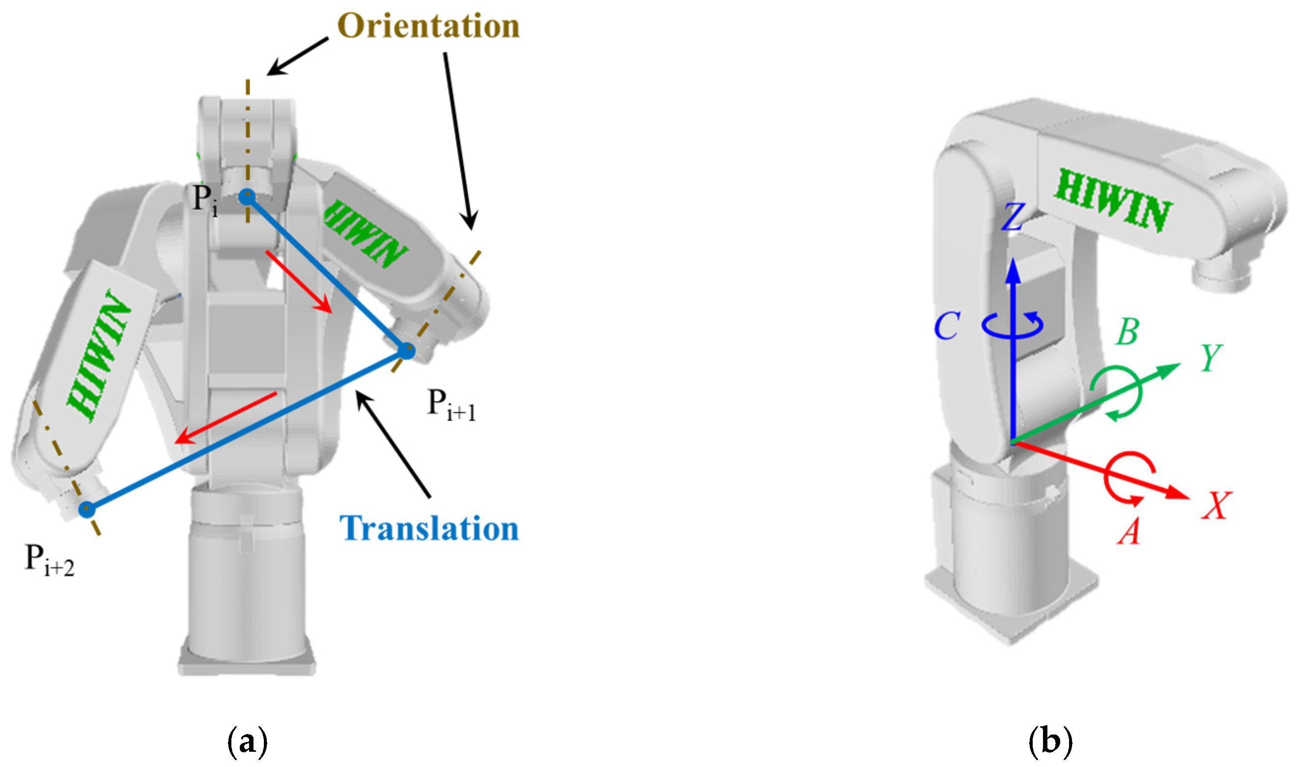
Point-to-point (P2P) and linear motion are the two most common types of robot trajectories. P2P is often used in pick-and-place applications. For P2P motion, only the initial and final positions are set; the trajectory is not specified. Linear motion requires designing an end-effector trajectory in the task space. The interpolated points at the end-effector are transformed into joint commands through inverse kinematics to achieve linear motion. Because velocity profiles designed for linear motion must include both translation and orientation commands, these commands should by synchronized in the interpolator (Figure 1a).

Table 1. Robot manipulator toolpath information.

No.	Type	Position (mm)			Orientation (deg)			Feed Rate (mm/s)
Pi	Linear	X 368.0	Y 0.00	Z 293.5	A 180.0	B 0.0	C 90.0	F 100.0
Pi+1	Linear	X 368.0	Y 200.0	Z 100.0	A 150.0	B 0.0	C 80.0	F 100.0
Pi+2	Linear	X 268.0	Y −200.0	Z −100.0	A −150.0	B −10.0	C 100.0	F 100.0

presents the toolpath information for Figure 1a, namely the position, orientation, and feed rate of the robot manipulator. The orientation is represented by A, B, and C, which indicate rotations around the X-, Y-, and Z-axes, respectively (Figure 1b).

A robot’s orientation is determined by a combination of rotations in the X, Y, and Z directions. Various methods can be used to describe the orientation of a rigid body, such as the Euler angle, roll–pitch–yaw angle, angle–axis representation, unit quaternion, and Cayley–Rodrigues parameter methods. In this study, the equivalent angle–axis representation was adopted; this method is similar to the quaternion method but involves fewer parameters. The rotation matrix in the equivalent angle–axis method can be represented by a unit vector (u) and an angle (ϕ) of revolution about the u vector.

The parameters u and ϕ are used to rotate the orientation of the end-effector from XYZ coordinates to X′Y′Z′ coordinates (Figure 2a). To obtain u and ϕ, rotation matrices for the XYZ and X′Y′Z′ coordinates are defined as R₁ and R₂. The matrices R₁ and R₂ can be obtained from two arbitrary orientation commands (A, B, C) on the toolpath. A general rotation matrix R can be calculated using Equation (1).

$$\begin{array}{l}\mathit{R}={\mathit{R}}_z\left(C\right){\mathit{R}}_y\left(B\right){\mathit{R}}_x\left(A\right)\\ =\left[\begin{array}{ccc}\cos C& -\sin C& 0\\ \sin C& \cos C& 0\\ 0& 0& 1\end{array}\right]\left[\begin{array}{ccc}\cos B& 0& \sin B\\ 0& 1& 0\\ -\sin B& 0& \cos B\end{array}\right]\left[\begin{array}{ccc}1& 0& 0\\ 0& \cos A& -\sin A\\ 0& \sin A& \cos A\end{array}\right]\\ =\left[\begin{array}{ccc}\cos C\cos B& -\sin C\cos A+\cos C\sin B\sin A& \sin C\sin A+\cos C\sin B\cos A\\ \sin C\cos B& \cos C\cos A+\sin C\sin B\sin A& -\cos C\sin A+\sin C\sin B\cos A\\ -\sin B& \cos B\sin A& \cos B\cos A\end{array}\right]\\ =\left[\begin{array}{ccc}{a}_{11}& a_{12}& a_{13}\\ a_{21}& a_{22}& a_{22}\\ a_{31}& a_{32}& a_{33}\end{array}\right]\end{array}$$

(1)

To convert a rotation matrix R back to an orientation command, the rotation matrix can be inverted by using Equations (2)–(4).

$$B=-{\sin }^{-1}\left(a_{31}\right)$$

(2)

$$A=\left\{\begin{array}{ll}\mathrm{atan}2\left(-a_{23},a_{22}\right)\hfill & if\cos B=0\hfill \\ \mathrm{atan}2\left(a_{32}/\cos B,a_{33}/\cos B\right)\hfill & otherwise\hfill \end{array}\right.$$

(3)

$$C=\left\{\begin{array}{ll}0\hfill & if\cos B=0\hfill \\ \mathrm{atan}2\left(a_{21}/\cos B,a_{11}/\cos B\right)\hfill & otherwise\hfill \end{array}\right.$$

(4)

To transform R₁ into R₂, R₁ must be multiplied by a rotation matrix R₁₂. The relationship between R₁ and R₂ can be expressed as follows, where R₁₂ represents the rotation matrix from R₁ to R₂:

$${\mathit{R}}_2={\mathit{R}}_{12}{\mathit{R}}_1$$

(5)

$${\mathit{R}}_{12}={\mathit{R}}_2{\mathit{R}}_1{}^{-1}={\mathit{R}}_{\varphi ,u}$$

(6)

The matrices R₁ and R₂ can be obtained from the orientation commands P_i and P_i+1. Matrix R₁₂ can then be calculated from Equation (6). However, the parameters u and ϕ are still unknown. The equivalent angle–axis representation can be employed to determine matrix R₁₂ by applying R_ϕ,u.

Figure 2. (a) Rotation in and (b) parameters of the equivalent angle–axis representation.

Figure 2. (a) Rotation in and (b) parameters of the equivalent angle–axis representation.

As shown in Figure 2b, the angle between the u vector and the i-k plane is represented by γ, and β represents the angle between the u′ vector and the k-axis. The projection of the u vector onto the i-, j-, and k-axes is represented by u_i, u_j, and u_k, respectively. The following relationships can be determined from Figure 2b:

$$\sin \gamma =u_j$$

(7)

$$\sin \beta =\frac{u_i}{\sqrt{u_i{}^2+u_k{}^2}}$$

(8)

$$\cos \gamma =\sqrt{u_i{}^2+u_k{}^2}$$

(9)

$$\cos \beta =\frac{u_k}{\sqrt{u_i{}^2+u_k{}^2}}$$

(10)

The rotation matrix R_ϕ,u, which describes the rotation ϕ around vector u, can be obtained as follows. First, vector u is rotated by angle γ on the i-axis to vector u′ located on the ik plane; the corresponding rotation matrix is represented by R_γ,i. Vector u′ is then rotated by angle −β on the j-axis to vector u″, which is located on the k-axis. This rotation matrix is represented by R_−β,j. Vector u″ is then rotated by ϕ on the k-axis; the rotation matrix is R_ϕ,k. The reverse sequence of rotations and their respective opposite angles can be expressed as R_β,j and R_−γ,i. After this sequence of rotations, the matrix R_ϕ,u can be represented as

$${\mathit{R}}_{\varphi ,u}={\mathit{R}}_{-\gamma ,i}{\mathit{R}}_{\beta ,j}{\mathit{R}}_{\varphi ,k}{\mathit{R}}_{-\beta ,j}{\mathit{R}}_{\gamma ,i}$$

(11)

$${\mathit{R}}_{\varphi ,u}=\left[\begin{array}{ccc}1& 0& 0\\ 0& c\gamma & s\gamma \\ 0& -s\gamma & c\gamma \end{array}\right]\left[\begin{array}{ccc}c\beta & 0& s\beta \\ 0& 1& 0\\ -s\beta & 0& c\beta \end{array}\right]\left[\begin{array}{ccc}c\varphi & -s\varphi & 0\\ s\varphi & c\varphi & 0\\ 0& 0& 1\end{array}\right]\left[\begin{array}{ccc}c\beta & 0& -s\beta \\ 0& 1& 0\\ s\beta & 0& c\beta \end{array}\right]\left[\begin{array}{ccc}1& 0& 0\\ 0& c\gamma & -s\gamma \\ 0& s\gamma & c\gamma \end{array}\right]$$

(12)

where sγ = sinγ, cγ = cosγ, sβ = sinβ, cβ = cosβ, sϕ = sinϕ, and cϕ = cosϕ.

By substituting Equations (7)–(10) into Equation (12), the following equation can be derived, where the abbreviation $v\varphi =1-\mathit{cos}\varphi$ is used:

$${\mathit{R}}_{\varphi ,u}=\left[\begin{array}{ccc}{u}_x{}^{2}v\varphi +c\varphi & u_x{u}_{\mathrm{y}}v\varphi -u_{\mathrm{z}}s\varphi & u_x{u}_{\mathrm{z}}v\varphi +u_{\mathrm{y}}s\varphi \\ u_x{u}_{\mathrm{y}}v\varphi +u_{\mathrm{z}}s\varphi & u_y{}^{2}v\varphi +c\varphi & u_y{u}_{\mathrm{z}}v\varphi -u_{\mathrm{x}}s\varphi \\ u_x{u}_{\mathrm{z}}v\varphi -u_{\mathrm{y}}s\varphi & u_y{u}_{\mathrm{z}}v\varphi +u_{\mathrm{x}}s\varphi & u_z{}^{2}v\varphi +c\varphi \end{array}\right]=\left[\begin{array}{ccc}{a}_{11}& a_{12}& a_{13}\\ a_{21}& a_{22}& a_{22}\\ a_{31}& a_{32}& a_{33}\end{array}\right]$$

(13)

The rotational angle and the unit vector can be obtained from Equations (14) and (15). After u and ϕ are obtained, ϕ can be used as the variable for interpolation.

$$\varphi =\pm {\cos }^{-1}\left[(a_{11}+a_{22}+a_{33}-1)/2\right]$$

(14)

$$u=\left[\begin{array}{c}{u}_x\\ u_y\\ u_z\end{array}\right]=\frac{1}{2s\varphi }\left[\begin{array}{c}{a}_{32}-a_{23}\\ a_{13}-a_{31}\\ a_{21}-a_{12}\end{array}\right]$$

(15)

As shown in Figure 1, the toolpath can be used to compute the translation distance L and the rotational angle ϕ determined using Equations (1)–(15). The S-shaped design method can be employed to generate a velocity profile for L or ϕ. The velocity profile can be divided into five phases (Figure 3) by Equation (16), where S_i represents the linear motion distance L or rotational angle ϕ of the end-effector.

$$\begin{array}{ll}{S}_1=V_{s}t+J_m{(t-t_0)}^3/6& t_0\le t<t_1\\ S_2=S_1+V_m\left(t-t_1\right)-0.5\cdot J_m\cdot \left[t_2{}^2\left(t-t_1\right)-t_2\left(t^2-t_1{}^2\right)+\left(t^3-t_1{}^3\right)/3\right]& t_1\le t<t_2\\ S_3=S_2+V_m\left(t-t_2\right)& t_2\le t<t_3\\ S_4=S_3+V_m\left(t-t_3\right)-J_m\left(t-t_3\right)/6& t_3\le t<t_4\\ S_5=S_4+V_e\left(t_5-t\right)+0.5\cdot J_m\cdot \left[t_5{}^2\left(t-t_4\right)-t_5\left(t^2-t_4{}^2\right)+\left(t^3-t_4{}^3\right)/3\right]& t_4\le t<t_5\end{array}$$

(16)

where J_m represents the maximum jerk, V_m represents the maximum feed rate, and V_s and V_e represent initial and final velocity (usually 0), respectively.

For example, consider the toolpath from P_i to P_i+1 for the position command for translation from (368, 0, 293.5) to (368, 200, 100) and the orientation command for rotation from (180, 0, 90) to (150, 0, 80). The interpolation should simultaneously plan both the translation and orientation commands.

Table 2. Constraints on interpolation parameters.

Parameter	Unit	Value
Trr	s	0.1
Vlf	mm/s	100
Vof	deg/s	100
Jlm	mm/s3	10,000
Jom	deg/s3	2000

presents the constraints on the interpolation parameters, where V_lf and V_of represent the maximum feed rate for translation and orientation, respectively, and J_lm and J_om represent the maximum jerk for translation and orientation, respectively. The velocity profile for the translation is planned first; Equation (17) is used to determine if the maximum jerk limit J_lm is exceeded. If so, the acceleration time can be adjusted using Equation (18), and the orientation can then be planned in accordance with the translation results. If the angular jerk still does not exceed the limit, planning is complete. However, if the angular jerk exceeds the limit, orientation must be planned first, and translation must be allocated afterwards in the same manner. In this example, the translation distance is 278.28 mm and the rotational angle is 31.58°; the results indicate that translation can be planned first.

$$J_m=V_m/T_{rr}{}^2$$

(17)

$$T_{rr}=\sqrt{V_m/J_m}$$

(18)

$${}_6{}^0\mathit{R}=\left[\begin{array}{cccc}& & & P_x\\ & {\mathit{R}}_{\varphi ,u}{\mathit{R}}_1& & P_y\\ & & & P_z\\ 0& 0& 0& 1\end{array}\right]$$

(19)

Figure 4 reveals that the resulting single program command achieves both translation and orientation. After the interpolation points (P_x, P_y, P_z) and the rotation matrix (R_ϕ,uR₁) for each sampling period are obtained, they can be substituted into Equation (19) to obtain the rotation matrix (${}_6{}^0\mathit{R}$). The joint commands can then be solved through inverse kinematics and used to command the motor drives, achieving synchronized translation and orientation for linear motion.

3. Corner Smoothing

In addition to single-line segment motion in positioning applications, corner interpolation must also be considered for tracking multi-line segment motion in polishing and grinding applications. Corner smoothing techniques can be employed to improve machining efficiency and reduce vibration at junctions. The motion of end-effector translation and orientation should be designed to ensure smoothness and continuity throughout the entire trajectory. Conventional methods for generating a smooth trajectory without excessive ACC/DEC can be categorized as ADBI and ADAI methods [5]. The ADBI method constrains the acceleration and the jerk of the trajectory; this prevents specifying the corner tolerance. However, the ADBI method can cause velocity discontinuities at block junctions, which can result in vibration. As shown in Figure 5, the feed rate (tangential velocity) is distributed across x- and y-axes in accordance with the direction of movement. The axis velocities V_x and V_y at the junction are not continuous.

The ADAI method, in which digital convolution is used eliminate velocity discontinuities on each axis, can resolve this problem (Figure 6). Corner tolerance occurs because the velocities of blocks N₁ and N₂ overlap. Digital convolution is performed using Equation (20), where $N=\tau /T_s$, $T_s$ represents the sample time and $\tau$ represents the time constant of the ACC/DEC. The input signal $x\left(k{T}_s\right)$ represents a velocity command.

$$y\left(k{T}_s\right)=\frac{1}{N}{\displaystyle \sum _{i=0}^{N-1}x\left[\left(k-i\right)T_s\right]}$$

(20)

Although the ADAI method is commonly used for interpolators, its applicability is limited because it can only be applied to the entire trajectory; the tolerance for each corner cannot be specified. To achieve both corner smoothing and a specified tolerance function, this paper proposes a VPO algorithm that calculates the overlapping time of line segments to produce blended S-shaped ACC/DEC profiles. This approach improves cycle times and enables the trajectory to be systematically designed to meet different accuracy requirements.

An example of the overlapping time of line segments is presented in Figure 7, which depicts two identical blocks with velocity blending. First, blocks 1 and 2 are planned using S-shaped ACC/DEC. Block 2 is then blended into block 1, and T_ol is the overlapped area of the two blocks; this represents as overlapping time. To calculate the overlapping time, the OVLP parameter is defined as a percentage. If OVLP is 100%, the overlapping time is 2T_rr, and the junction of the two blocks occurs exactly at half of V_m. Therefore, 2V_c is equal to V_m. The relationship between the OVLP parameter and the velocity can be expressed as follows:

$$OVLP=\frac{2V_c}{V_m}\times 100\%$$

(21)

where V_c is the velocity junction between the two blocks.

The relationship between V_c and the overlapping time (T_ol) can be calculated using the A–T diagram in Figure 7. For an S-shaped velocity profile, A_m = V_m/T_rr, where A_m represents the maximum acceleration and T_rr is equal to the time of acceleration from 0 to A_m within the ACC/DEC period. A_c represents V_c at the junction and can be calculated using Equation (22).

$$A_c=\frac{A_m{T}_{ol}}{2T_{rr}}=\frac{V_m{T}_{ol}}{2T_{rr}^2}$$

(22)

The parameter V_c can be calculated by integrating the area of the A–T diagram and is given as follows:

$$V_c=\frac{A_c{T}_{ol}}{4}$$

(23)

By substituting Equation (22) into Equation (23), V_c can be represented by

$$V_c=\frac{V_m{T}_{ol}{}^2}{8T_{rr}^2}$$

(24)

T_ol can be calculated from OVLP by substituting Equation (21) into Equation (24) as follows:

$$T_{ol}=\sqrt{\frac{8V_c{T}_{rr}{}^2}{V_m}}=2T_{rr}\sqrt{\frac{OVLP}{100}}$$

(25)

Equation (25) indicates that T_ol is a function of OVLP and T_rr. Because T_rr is already known, OVLP can be adjusted to quickly control the smoothing of the corner, improving the cycle time. The velocity profiles on the x- and y-axes for different values of OVLP are shown in Figure 8c,d, in which OVLP is equal to 0% and 80%, respectively. When OVLP is 80%, the starting time for the N₂ block moves forward by T_ol on both the x- and y-axes. The VPO approach ensures that the velocity is continuous at the junction for each axis, and the cycle time decreases from 1.6 to 1.38 s. However, a corner tolerance can occur at the junction if OVLP increases (Figure 8a). The next section describes the derivation of the CTC equation, which can be used to systematically evaluate the corner tolerance on the basis of the overlapping time.

4. CTC Algorithm

A corner tolerance occurs when the velocity profiles of line segments overlap. The maximum corner tolerance occurs at half of the overlapping time (T_ol/2). Figure 9 presents the overlapping area of Figure 7. Figure 9a shows the trajectory of block 1 and block 2 at the corner after overlapping; P₁, P₄, and P₃ and are produced from P₁, P₂, and P₃. Here, the distance from P₂ to P₄ is the maximum corner tolerance. Figure 9b presents the velocity profiles of block 1 and block 2 and the overlapped velocity profile, where V_x1 and V_x2 represent the velocity profiles on the x-axis of block 1 and block 2, respectively, and the blue solid line formed by P₁, P₄, and P₃ represents the velocity profile of the two blocks after overlapping. The maximum corner tolerance occurs at point P₄.

The three-dimensional corner tolerance (ε) can be calculated from the x, y, and z parameters as follows:

$$\epsilon =\sqrt{{\epsilon }_x{}^2+{\epsilon }_y{}^2+{\epsilon }_z{}^2}$$

(26)

In Figure 9a, ε_x1 is the distance from P₁ to P₂ for block 1 in the x direction and can be calculated by integrating the area of BDE in Figure 9b; this area represents the distance from P₅ to P₂ in the X direction. To obtain ε_x1, the S₁ term in Equation (16) can be replaced by Equation (27), where t is substituted with T_ol/2 and J is substituted with J_x1, obtaining Equation (28).

$$S=J{t}^3/6$$

(27)

$${\epsilon }_{x1}=\frac{J_{x1}{T}_{ol}{}^3}{48}$$

(28)

When considering the overlap effect, P₅ should move to a distance projected on the x-axis relative to P₄, represented as ${\epsilon }_{x2}$. The value of ${\epsilon }_{x2}$ represents the area under ACD and is given by Equation (29), where J_x2 represents the jerk of N₂ along the x direction.

$${\epsilon }_{x2}=\frac{J_{x2}{T}_{ol}{}^3}{48}$$

(29)

The distance between P₄ and P₂ on the X-axis is represented by ${\epsilon }_x$ and can be calculated using the following equation.

$${\epsilon }_x={\epsilon }_{x1}-{\epsilon }_{x2}$$

(30)

Here, ${\epsilon }_x$ represents the corner tolerance $\epsilon$ projected on the x-axis. Similarly, the corner tolerance components in the y and z directions can be calculated using Equations (31) and (32).

$${\epsilon }_y={\epsilon }_{y1}-{\epsilon }_{y2}$$

(31)

$${\epsilon }_z={\epsilon }_{z1}-{\epsilon }_{z2}$$

(32)

where ${\epsilon }_{y1}=J_{y1}{T_{ol}}^3/48$, ${\epsilon }_{y2}=J_{y2}{T_{ol}}^3/48$, ${\epsilon }_{z1}=J_{z1}{T_{ol}}^3/48$, and ${\epsilon }_{z2}=J_{z2}{T_{ol}}^3/48$.

The relationship between T_ol and $\epsilon$ can be obtained by substituting Equations (30)–(32) into (26).

$$\epsilon =\sqrt{{\left(\frac{\left(J_{x1}-J_{x2}\right)T_{ol}{}^3}{48}\right)}^2+{\left(\frac{\left(J_{y1}-J_{y2}\right)T_{ol}{}^3}{48}\right)}^2+{\left(\frac{\left(J_{z1}-J_{z2}\right)T_{ol}{}^3}{48}\right)}^2}$$

(33)

Summing the squares of Equation (33) produces Equation (34), where ${\left(J_{x1}-J_{x2}\right)}^2+{\left(J_{y1}-J_{y2}\right)}^2+{\left(J_{z1}-J_{z2}\right)}^2$ is abbreviated to J_xyz

$${\epsilon }^2=\frac{T_{ol}{}^6{J}_{xyz}}{{48}^2}$$

(34)

After jerk and corner tolerance have been determined, T_ol can be obtained using Equation (35), and the CTC equation can be expressed as follows:

$$T_{ol}=\sqrt[6]{\frac{{48}^2{\epsilon }^2}{J_{xyz}}}$$

(35)

In Section 2, the S-shaped design method was adopted to plan the translation and orientation. In Section 3, the VPO method was applied to plan a line segment, solving the discontinuity problem. By contrast with the conventional ADAI approach, the VPO method can explicitly specify the corner tolerance for each corner. Finally, the designed velocity profile can be integrated to obtain positions and substituted into Equation (19) to generate the command points for each axis, completing the interpolation process.

5. Results of Simulations and Experiments

Experiments were conducted to evaluate the effectiveness of the proposed algorithm for the HIWIN RT605 robot manipulator. The robotic equipment was equipped with a PC-based controller with a real-time operating system enabling multitasking; the sampling time was set to 1 ms. The software included a human–machine interface, a numerical control (NC) interpreter, a kinematics module, an interpolator, and a multiaxis contour trajectory motion system. Figure 10 presents the hardware used in the experiment, which comprised Sanyo Denki servo motors and drivers. The six-axis servo drives were commanded through the EtherCAT protocol to ensure that the robotic equipment moved synchronously.

5.1. Simulation Results for Difference OVLP Parameters

To evaluate the VPO methodology, a simple polygon trajectory comprising six line segments was tested (Figure 11a). The corresponding NC code is listed in

Table 3. NC code for simple polygon.

No.	Position (mm)			Orientation (deg)			Case 1	Case 2	Case 3	Feed Rate (mm/s)
	X	Y	Z	A	B	C	OVLP (%)	OVLP (%)	Corner Tolerance (mm)
O	468	−100	0	180	0	0	-	-	-	-
A	468	0	0	170	10	10	100	90	4.2	150
B	368	0	0	150	20	30	100	80	3.4	150
C	350	100	0	180	0	0	100	0	2.6	150
D	268	0	0	−160	10	−10	100	60	0	150
E	268	−100	0	−170	20	−30	100	70	4.0	150
O	468	−100	0	180	0	0	-	-	-	-

, and the interpolation parameters are provided in

Table 4. Kinematic constraints of robot manipulator.

Parameters	X-Axis (mm)	Y-Axis (mm)	Z-Axis (mm)	Orientation (deg)
Velocity (mm/s, deg/s)	2000	2000	2000	500
Acceleration (mm/s2, deg/s2)	3500	3500	3500	2000
Jerk (mm/s3, deg/s3)	50,000	50,000	50,000	30,000

. The trajectory planning process must satisfy both kinematic constraints and tolerance constraints, and simultaneous translation and orientation were required. The velocity and acceleration profiles of the tool center point (TCP) at a full stop in Case 1 and in Case 2 are shown in Figure 12. In the full stop scenario, movement stops completely at each corner. Although this case has no corner tolerance, it has the longest cycle time of approximately 6.37 s. In Case 1, all of the OVLP parameters were set to 100%, reducing the cycle time from 6.37 to 5.12 s (19.6%). However, the corner tolerance was larger than in other cases. In Case 2, the OVLP parameters were adjusted to control the smoothness of each corner. This method is more flexible than the ADAI method. The corner smoothing results for each case are presented in Figure 11b–f. In the VPO algorithm, the parameter OVLP controlled the level of overlap in the velocity profiles. Higher OVLP values result in smoother corner trajectories and shorter cycle times. However, increasing the OVLP parameter leads to a larger corner tolerance.

5.2. Simulation Results for the CTC Method

To confirm that the VPO algorithm not only satisfies the kinematic constraints but can also be used to specify the tolerance at the corner of the corner, another experiment, Case 3, was performed. The NC code for Case 3 is shown in Table 3. The velocity and acceleration of the TCP for Case 3 are shown in Figure 13a. The feed rate reached 150 mm/s with a maximum acceleration of −1430 mm/s² and a cycle time of 5.45 s. Figure 13b presents the profiles of axial velocity, axial acceleration, and axial jerk. The maximum axial acceleration and jerk occurred on the y-axis and were −1684 mm/s² and 20,000 mm/s³, respectively. For orientation planning, the rotational angles were calculated from Equations (1), (6), (14) and (15), obtaining 17.8°, 33.2°, 49.7°, 25.1°, 22.2°, and 38.6°. The results for the x, y, and z rotations are presented in Figure 14. The maximum velocity was 48.48 deg/s, the maximum acceleration was 509.7 deg/s², and the maximum jerk was 5309 deg/s³. Hence, the position and orientation of the end-effectors of the robot manipulator satisfy the kinematic constraints. Finally, the rotation matrix and position were substituted back into Equation (19), and the joint commands were obtained through inverse kinematics. Figure 15 presents the joint commands, angular velocity, angular acceleration, and angular jerk. The maximum values of velocity, acceleration, and jerk are −69.7 deg/s, −932 deg/s², and −9701 deg/s³, respectively.

To validate the effectiveness of the CTC equation in the VPO algorithm, the results for Case 3 (Table 3) were analyzed. The corner tolerance is the shortest distance from the sharp corner to the ultimate trajectory. By inputting the overlapping time calculated with the CTC equation to the VPO algorithm, the corner tolerance at each corner can be correctly constrained within the specified tolerance. When the corner tolerances of A, B, C, D, and E on the trajectory in Figure 16a were set to 4.2, 3.4, 2.6, 0, and 4.0 mm, respectively, the resulting trajectories at each corner in Figure 16b–f satisfied these constraints with overlapping times of 0.237, 0.226, 0.181, 0, and 0.22 s, respectively. Hence, the simulation results confirm that the proposed VPO algorithm, unlike the conventional ADAI approach, enables separately setting corner tolerances at each corner to satisfy the specified constraints.

5.3. Experimental Comparison of VPO and ADAI

The simulation results discussed in the previous sections clearly indicate that the OVLP parameter affects the cycle time and corner tolerance. In this section, experiments were conducted for the HIWIN robot RT605 using real trajectories; the results are shown in Figure 17. Trajectories were obtained using the VPO method and the conventional interpolation method (ADAI). The feed rate, tolerance, and maximum acceleration of the TCP were the same for both algorithms. For the ADAI method with a time constant of 500 ms and the VPO method with the acceleration time set to 0.25 s and OVLP to 74%, the contour and tracking errors in the x, y, and z directions were almost identical (Figure 17c,d). However, the cycle time of the VPO method was only 8.98 s, 10.6% less than that of the ADAI method. However, if the acceleration time and OVLP parameter in the VPO method were adjusted to 0.35 s and 58% (to maintain a similar cycle time), the contour error [25] at point A decreased from 0.1841 mm to 0.1566 mm, a reduction of approximately 15.22% (Figure 17e,f). This result indicates that the trajectory planning of the VPO algorithm is excellent.

Table 5. Cycle times of the VPO and ADAI trajectories with approximately equal maximum contour and tracking errors.

Case	Feed Rate (mm/s)	VPO	ADAI	Cycle Time
		Acceleration Time (s)/ OVLP (%)	Maximum Acceleration (mm/s)/ Time Constant (ms)	ADAI (s)/ VPO (s)/ Reduced (%)
Case A	100	0.25/74	1200/500	10.05/8.98/10.60
Case B	100	0.35/81	1600/700	10.11/9.18/9.19
Case C	150	0.28/85	1600/600	7.32/6.42/12.30

reveals that the cycle time of the VPO method was 9.19–12.30% lower than that of the ADAI method. For Cases A, B, and C, the cycle times of the VPO method were approximately 8.98, 9.18, and 6.42 s, respectively.

Table 6. Contour error of the VPO and ADAI trajectories with approximately equal cycle times.

Case	Feed Rate (mm/s)	VPO	ADAI	Point A Contour Error
		Acceleration Time (s)/ OVLP (%)	Maximum Acceleration (mm/s)/ Time Constant (ms)	ADAI (mm)/ VPO (mm)/ Reduced (%)
Case D	100	0.35/58	1200/500	0.1841/0.1566/15.22
Case E	100	0.44/81	1600/700	0.1826/0.1693/7.28
Case F	150	0.33/84	1600/600	0.2005/0.1883/6.08

reveals that the contour error in the VPO method was 6–15% lower than that of the ADAI method. For Cases D, E, and F, the maximum contour errors of the VPO method were approximately 0.1566, 0.1693, and 0.1883 mm, respectively. The statistical results presented in Table 5 and Table 6 demonstrate that the VPO method outperforms ADAI in terms of both feasibility and performance.

6. Conclusions

This study proposed a VPO algorithm for designing robotic interpolators that uses the velocity overlap method on each axis to remove the discontinuities caused by projecting the velocity profile of the TCP onto each axis. A superior balance between smoothness and cycle time can be achieved by adjusting the overlapping time. This paper described the derivation of the CTC equation, which enables using the VPO method to individually control the tolerance for each corner. Other interpolation design methods, such as the conventional ADAI approach, do not incorporate these features. The experimental results indicate that the VPO algorithm outperformed the ADAI method by reducing the cycle time by 6.08–15.22% if the parameters of the methods were adjusted to obtain approximately equal contour error. Experiments were also conducted to confirm that the contour errors could be reduced by 9.19–12.30% if the cycle times of both algorithms were adjusted to be approximately equal. The results confirm the effectiveness of the VPO method.

References

1. Zhang, Y.; Rao, P.; Jia, L.; Chen, X. Dim moving infrared target enhancement based on precise trajectory extraction. Infrared Phys. Technol. 2023, 128, 104374. [Google Scholar] [CrossRef]
2. Ni, H.; Zhang, C.; Chen, Q.; Ji, S.; Hu, T.; Liu, Y. A novel time-rounding-up-based feedrate scheduling method based on S-shaped ACC/DEC algorithm. Int. J. Adv. Manuf. Technol. 2019, 104, 2073–2088. [Google Scholar] [CrossRef]
3. Liu, T.; Wang, J.; Yang, B.; Wang, X. NGDNet: Nonuniform Gaussian-label distribution learning for infrared head pose estimation and on-task behavior understanding in the classroom. Neurocomputing 2021, 436, 210–220. [Google Scholar] [CrossRef]
4. Rossi, C.; Savino, S. Robot Trajectory Planning by Assigning Positions and Tangential Velocities. Robot. Comput.-Integr. Manuf. 2013, 29, 139–156. [Google Scholar] [CrossRef]
5. Tsai, M.-S.; Huang, Y.-C. A Novel Integrated Dynamic Acceleration/Deceleration Interpolation Algorithm for a CNC Controller. Int. J. Adv. Manuf. Technol. 2016, 87, 279–292. [Google Scholar] [CrossRef]
6. Fang, S.; Cao, J.; Zhang, Z.; Zhang, Q.; Cheng, W. Study on High-Speed and Smooth Transfer of Robot Motion Trajectory Based on Modified S-Shaped Acceleration/Deceleration Algorithm. IEEE Access 2020, 8, 199747–199758. [Google Scholar] [CrossRef]
7. Wang, W.; Tao, Q.; Cao, Y.; Wang, X.; Zhang, X. Robot Time-Optimal Trajectory Planning Based on Improved Cuckoo Search Algorithm. IEEE Access 2020, 8, 86923–86933. [Google Scholar] [CrossRef]
8. Ahn, J.; Chung, W.; Jung, C. Realization of Orientation Interpolation of 6-Axis Articulated Robot Using Quaternion. J. Cent. South Univ. 2012, 19, 3407–3414. [Google Scholar] [CrossRef]
9. Kong, M.-X.; Ji, C.; Chen, Z.-S.; Li, R. Application of Orientation Interpolation of Robot Using Unit Quaternion. In Proceedings of the 2013 IEEE International Conference on Information and Automation (ICIA), Harbin, China, 26–28 August 2013; pp. 384–389. [Google Scholar]
10. Pu, Y.; Shi, Y.; Lin, X.; Hu, Y.; Li, Z. C2-Continuous Orientation Planning for Robot End-Effector with B-Spline Curve Based on Logarithmic Quaternion. Math. Probl. Eng. 2020, 2020, e2543824. [Google Scholar] [CrossRef]
11. Sencer, B.; Ishizaki, K.; Shamoto, E. High Speed Cornering Strategy with Confined Contour Error and Vibration Suppression for CNC Machine Tools. CIRP Ann. 2015, 64, 369–372. [Google Scholar] [CrossRef]
12. Tajima, S.; Sencer, B. Accurate real-time interpolation of 5-axis tool-paths with local corner smoothing. Int. J. Mach. Tools Manuf. 2019, 142, 1–15. [Google Scholar] [CrossRef]
13. Li, H.; Wu, W.J.; Rastegar, J.; Guo, A. A real-time and look-ahead interpolation algorithm with axial jerk-smooth transition scheme for computer numerical control machining of micro-line segments. Proc. Inst. Mech. Eng. Part B J. Eng. Manuf. 2019, 233, 2007–2019. [Google Scholar] [CrossRef]
14. Bi, Q.; Huang, J.; Lu, Y.; Zhu, L.; Ding, H. A general, fast and robust B-spline fitting scheme for micro-line tool path under chord error constraint. Sci. China Technol. Sci. 2019, 62, 321–332. [Google Scholar] [CrossRef]
15. Song, D.N.; Ma, J.W.; Zhong, Y.G.; Yao, J.J. Global smoothing of short line segment toolpaths by control-point-assigning-based geometric smoothing and FIR filtering-based motion smoothing. Mech. Syst. Signal Process. 2021, 160, 107908. [Google Scholar] [CrossRef]
16. Sun, S.; Lin, H.; Zheng, L.; Yu, J.; Hu, Y. A Real-Time and Look-Ahead Interpolation Methodology with Dynamic B-Spline Transition Scheme for CNC Machining of Short Line Segments. Int. J. Adv. Manuf. Technol. 2016, 84, 1359–1370. [Google Scholar] [CrossRef]
17. Han, J.; Jiang, Y.; Tian, X.; Chen, F.; Lu, C.; Xia, L. A Local Smoothing Interpolation Method for Short Line Segments to Realize Continuous Motion of Tool Axis Acceleration. Int. J. Adv. Manuf. Technol. 2018, 95, 1729–1742. [Google Scholar] [CrossRef]
18. Sun, J.; Han, X.; Zuo, Y.; Tian, S.; Song, J.; Li, S. Trajectory Planning in Joint Space for a Pointing Mechanism Based on a Novel Hybrid Interpolation Algorithm and NSGA-II Algorithm. IEEE Access 2020, 8, 228628–228638. [Google Scholar] [CrossRef]
19. Chen, C.-S.; Chen, S.-K.; Lai, C.-H. Real-Time Coplanar NURBS Curve Fitting and Interpolation for 6-DOF Robot Arm. In Proceedings of the 2015 International Conference on Advanced Robotics and Intelligent Systems (ARIS), Taipei, Taiwan, 29–31 May 2015; pp. 1–6. [Google Scholar]
20. Ni, H.; Yuan, J.; Ji, S.; Zhang, C.; Hu, T. Feedrate scheduling of NURBS interpolation based on a novel jerk-continuous ACC/DEC algorithm. IEEE Access 2018, 6, 66403–66417. [Google Scholar] [CrossRef]
21. Tajima, S.; Sencer, B. Global tool-path smoothing for CNC machine tools with uninterrupted acceleration. Int. J. Mach. Tools Manuf. 2017, 121, 81–95. [Google Scholar] [CrossRef]
22. Tajima, S.; Sencer, B. Online interpolation of 5-axis machining toolpaths with global blending. Int. J. Mach. Tools Manuf. 2022, 175, 103862. [Google Scholar] [CrossRef]
23. Tajima, S.; Sencer, B.; Shamoto, E. Accurate interpolation of machining tool-paths based on FIR filtering. Precis. Eng. 2018, 52, 332–344. [Google Scholar] [CrossRef]
24. Fang, J.; Li, B.; Zhang, H.; Ye, P. Real-time smooth trajectory generation for 3-axis blending tool-paths based on FIR filtering. Int. J. Adv. Manuf. Technol. 2023, 126, 3401–3416. [Google Scholar] [CrossRef]
25. Zhao, H.; Li, X.; Ge, K.; Ding, H. A Contour Error Definition, Estimation Approach and Control Structure for Six-Dimensional Robotic Machining Tasks. Robot. Comput.-Integr. Manuf. 2022, 73, 102235. [Google Scholar] [CrossRef]
Figure 1. Robot manipulator. (a) Translation and orientation of a trajectory. (b) Rotations A, B, and C around the X-, Y-, and Z-axes.
Applsci 13 08789 g001
Figure 3. S-shaped ACC/DEC profile.
Applsci 13 08789 g003
Figure 4. Planning result of a single program command (a) Translation. (b) Orientation.
Applsci 13 08789 g004
Figure 5. ADBI method.
Applsci 13 08789 g005
Figure 6. The ADAI method.
Applsci 13 08789 g006
Figure 7. Diagram of the VPO parameters.
Applsci 13 08789 g007
Figure 8. Comparison of velocity profile with OVLP equal to 80% and without OVLP. (a) Trajectory. (b) Tangential velocity. Velocities on the (c) x-axis and (d) y-axis.
Applsci 13 08789 g008
Figure 9. Schematic of corner tolerance. (a) Trajectory. (b) X-axis velocity profile.
Applsci 13 08789 g009
Figure 10. Hardware and software architecture of the experiment.
Applsci 13 08789 g010
Figure 11. Corner smoothing results with various OVLP parameters for the trajectory. (a) Entire trajectory. (b) Corner A. (c) Corner B. (d) Corner C. (e) Corner D. (f) Corner E.
Applsci 13 08789 g011
Figure 12. Velocity and acceleration profiles of the TCP for a simple polygon.
Applsci 13 08789 g012
Figure 13. Kinematic profile of the TCP and axial direction. (a) Velocity and acceleration. (b) Velocity, acceleration, and jerk.
Applsci 13 08789 g013
Figure 14. Simulation results for the orientation profile. (a) Position. (b) Velocity, acceleration, and jerk.
Applsci 13 08789 g014
Figure 15. Simulation results for the joint profile. (a) Position and angular velocity. (b) Angular acceleration and angular jerk.
Applsci 13 08789 g015
Figure 16. Corner tolerances in the CTC method. (a) Trajectory. (b) Corner A. (c) Corner B. (d) Corner C. (e) Corner D. (f) Corner E.
Applsci 13 08789 g016
Figure 17. Results of the star experiment. (a) Trajectory. (b) Velocity and acceleration profiles for Case A. Cycle times for Case A with the same (c) contour and (d) tracking errors. Comparison of (e) contour and (f) tracking errors for Case D with the same cycle time.
Applsci 13 08789 g017