
Investigation on Intelligent Early Warning of Rock Burst Disasters Using the PCA-PSO-ELM Model

Abstract
:1. Introduction
2. Model Principles and Methods
2.1. PCA
- Standardize the sample data and calculate the correlation matrix.
- Solve the eigenvalues and sort the principal components according to their magnitudes.
- Calculate the variance contribution rate of each principal component and select m (m < n) principal components based on the principle of the cumulative variance contribution rate reaching 85%.
- Calculate the correlation coefficient matrix and list the calculation formula of the principal components so that the dimensionality reduction of the original data can be achieved.
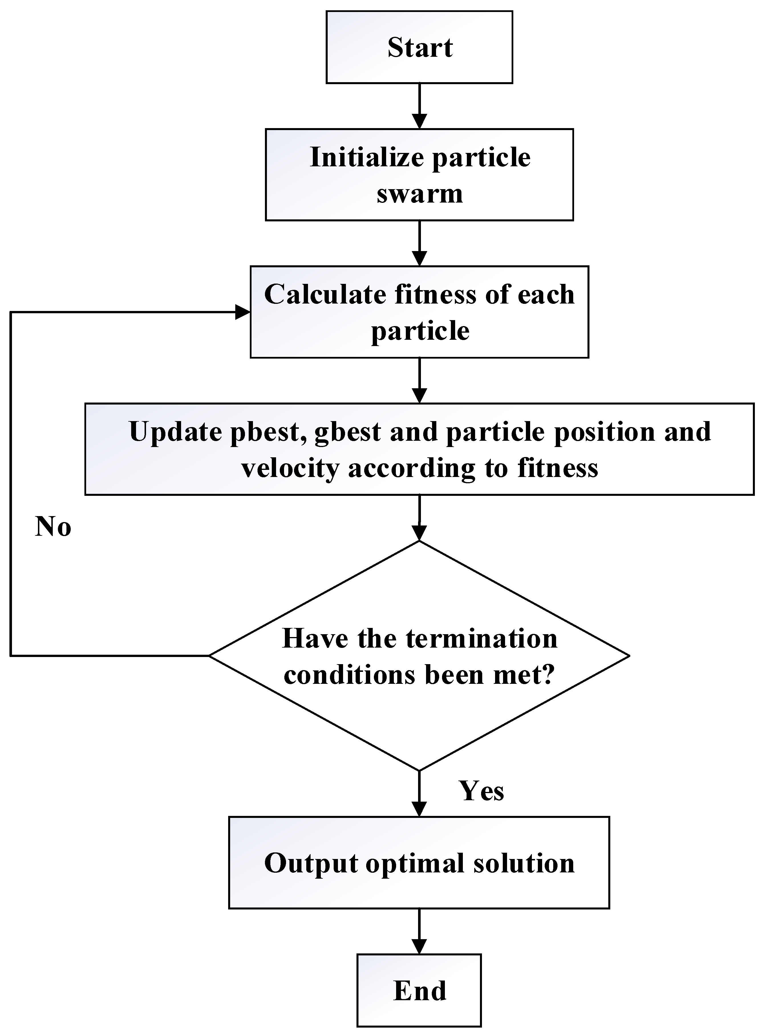
2.2. PSO Method
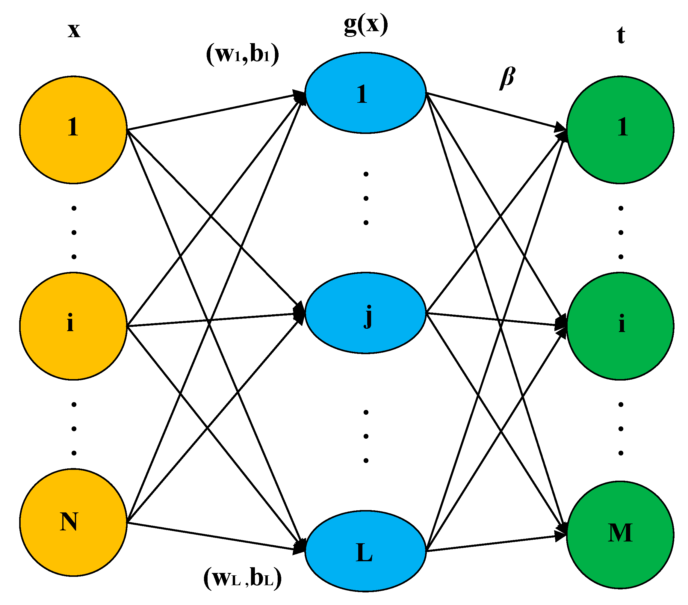
2.3. ELM
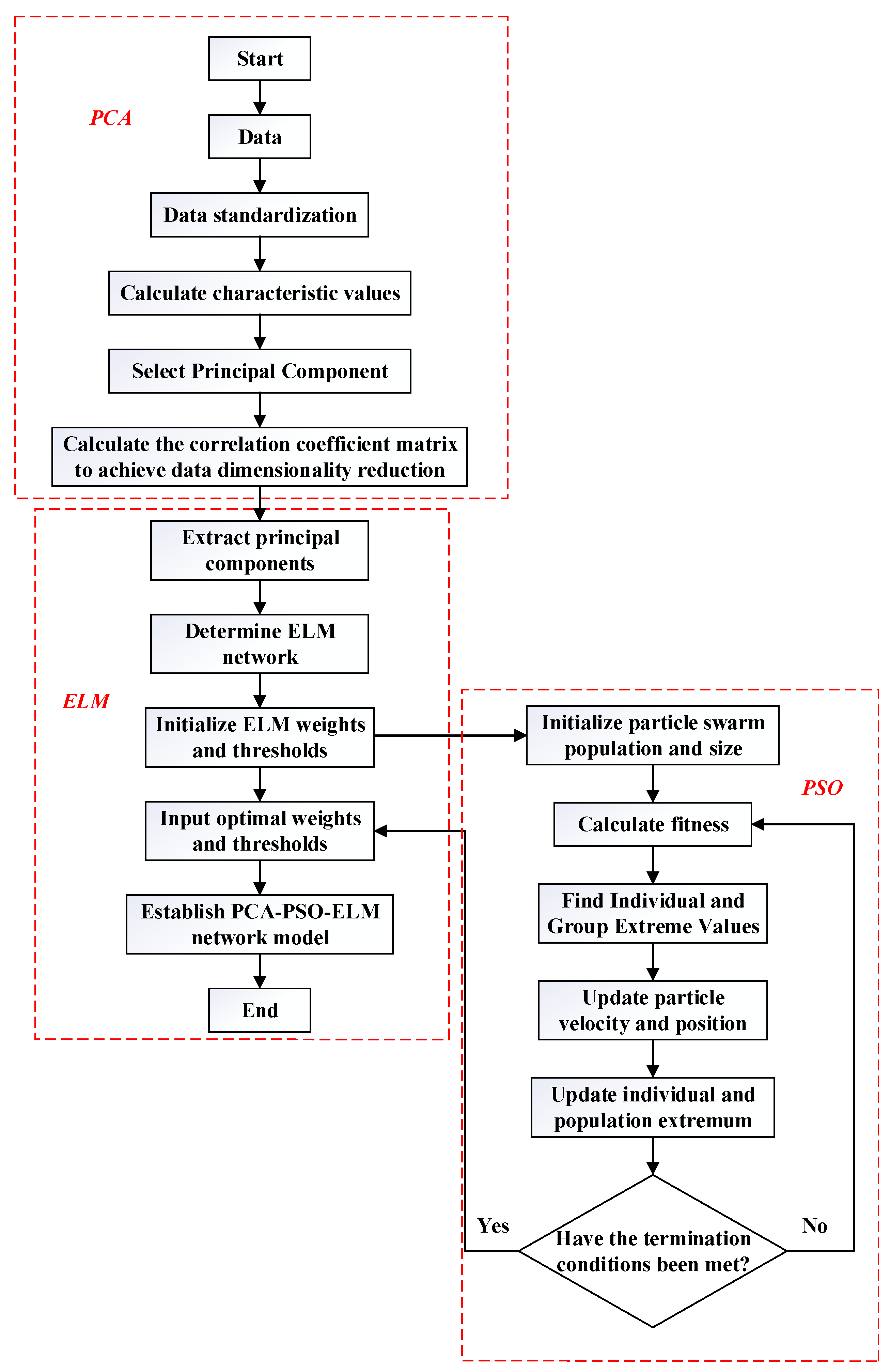
2.4. Combined Early Warning Model of PCA–PSO–ELM
3. Example Analysis
3.1. Early Warning Indicator System for Rock Bursts
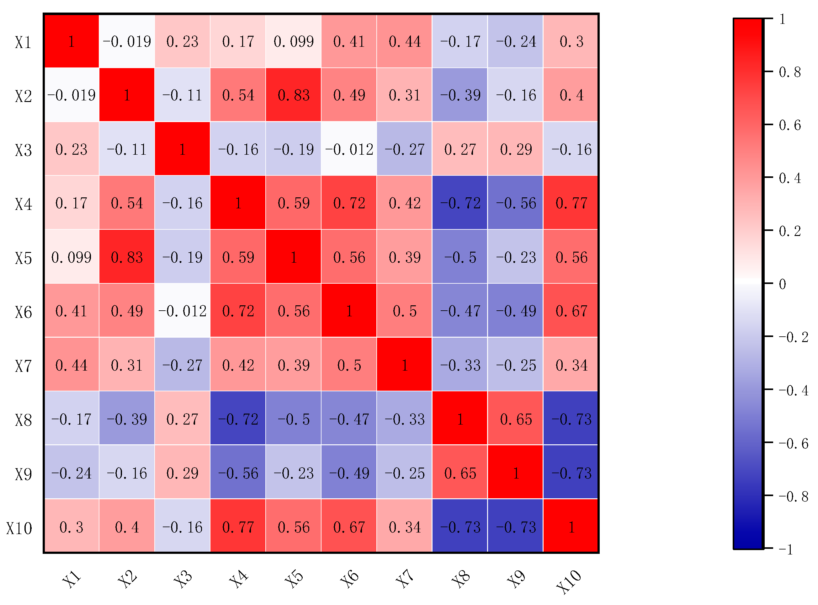
3.2. Principal Component Data Analysis
3.2.1. KMO Inspection and Bartlett Sphericity Test
3.2.2. Principal Component Extraction
3.3. Combined Early Warning Model of PCA–PSO–ELM for Rock Bursts
3.4. Results Analysis
4. Conclusions
- Taking the 10 factors that affected the occurrence of rock bursts in the Yanshitai Coal Mine as the main influencing factors, the PCA method was used to extract the dimension reduction feature information of the evaluation index, from which six principal components were extracted as the input vectors for extreme learning machine, eliminating the interaction between the various factors and simplifying the network structure of the model.
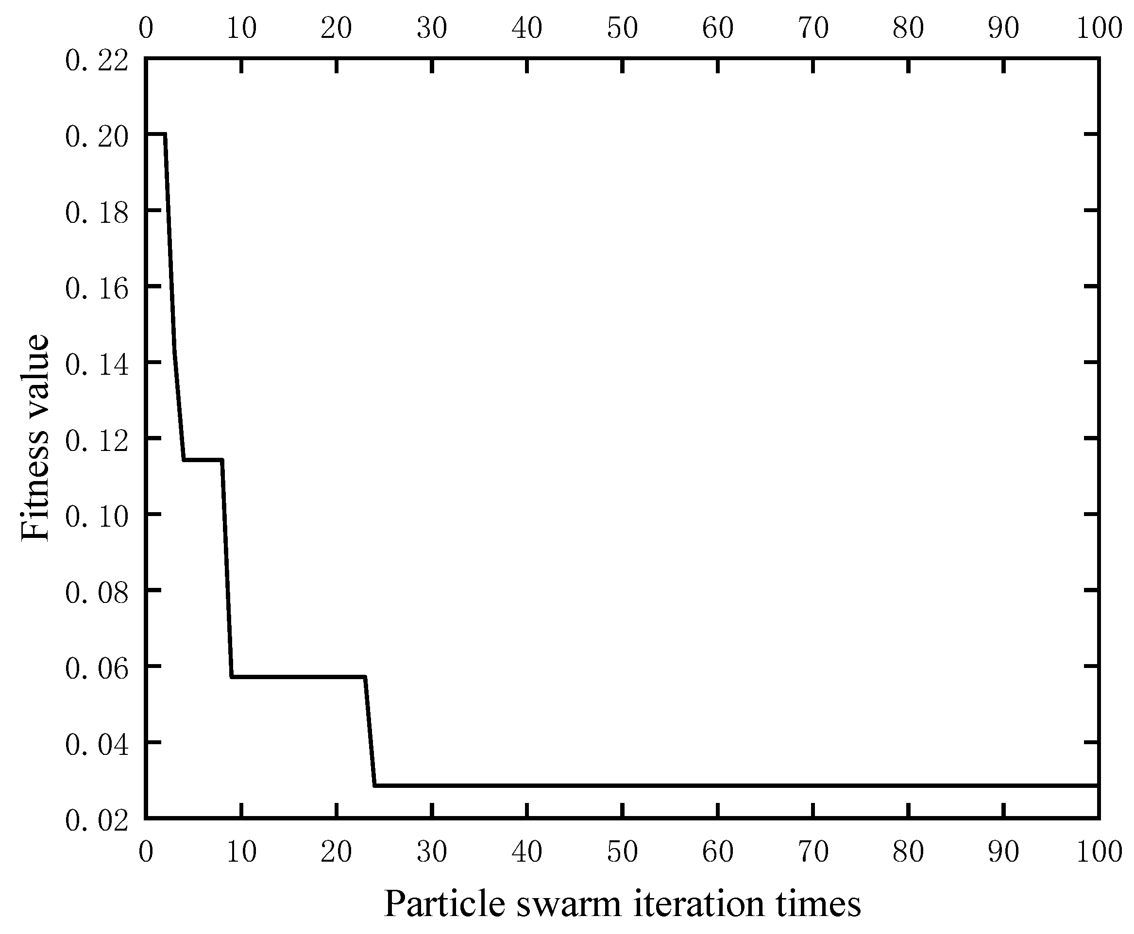
- Using the PSO algorithm, the initial weights and hidden layer neuron thresholds of the ELM were optimized. Therefore, a combined early warning PSO–ELM model for rock bursts was ultimately established, which overcame the disadvantage of randomness of the input weights and hidden layer thresholds of the ELM and enhanced the accuracy of the model prediction.
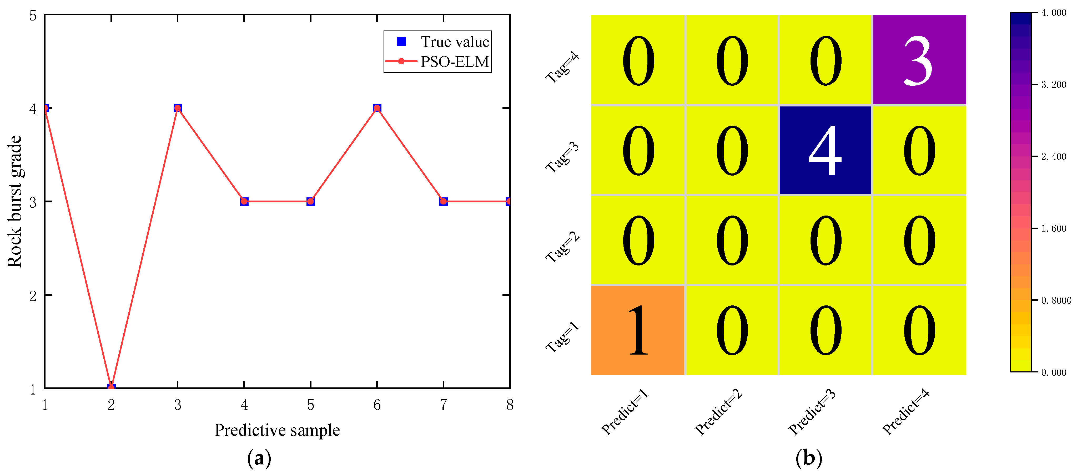
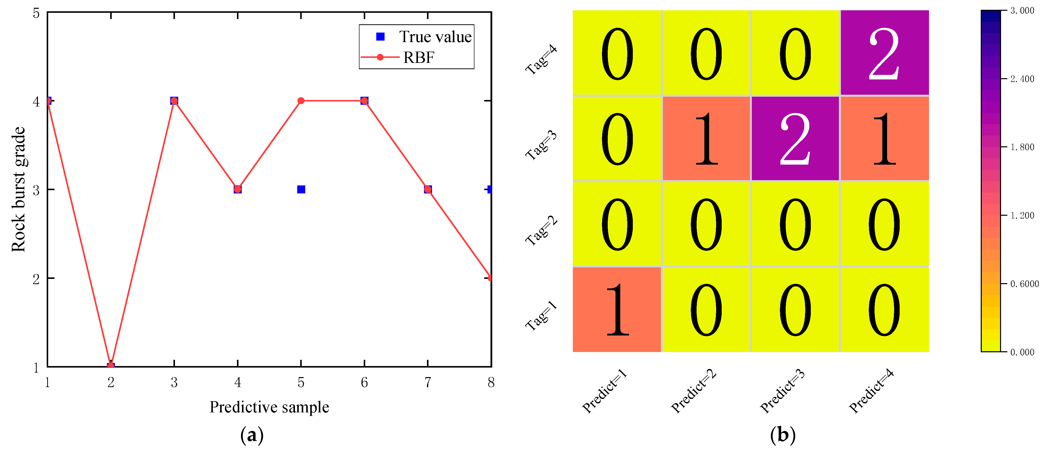
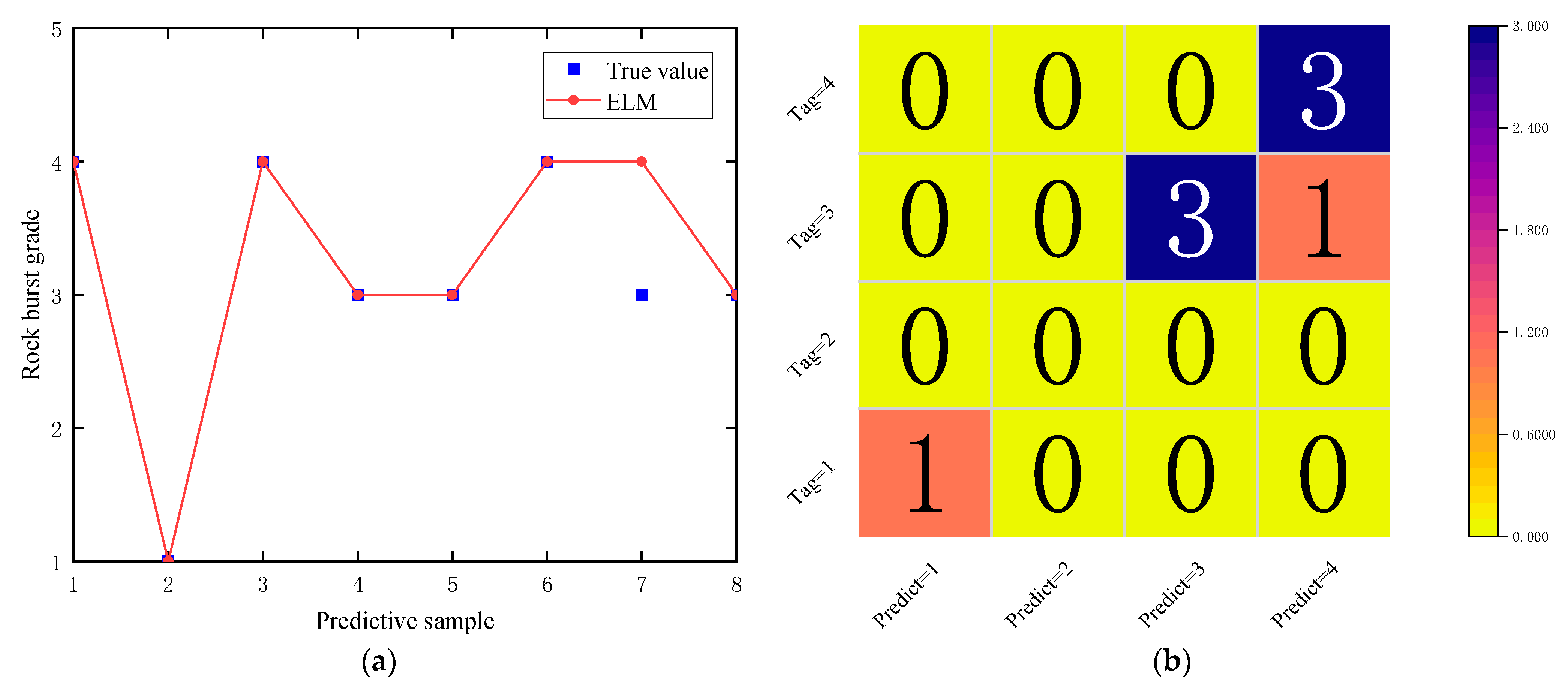
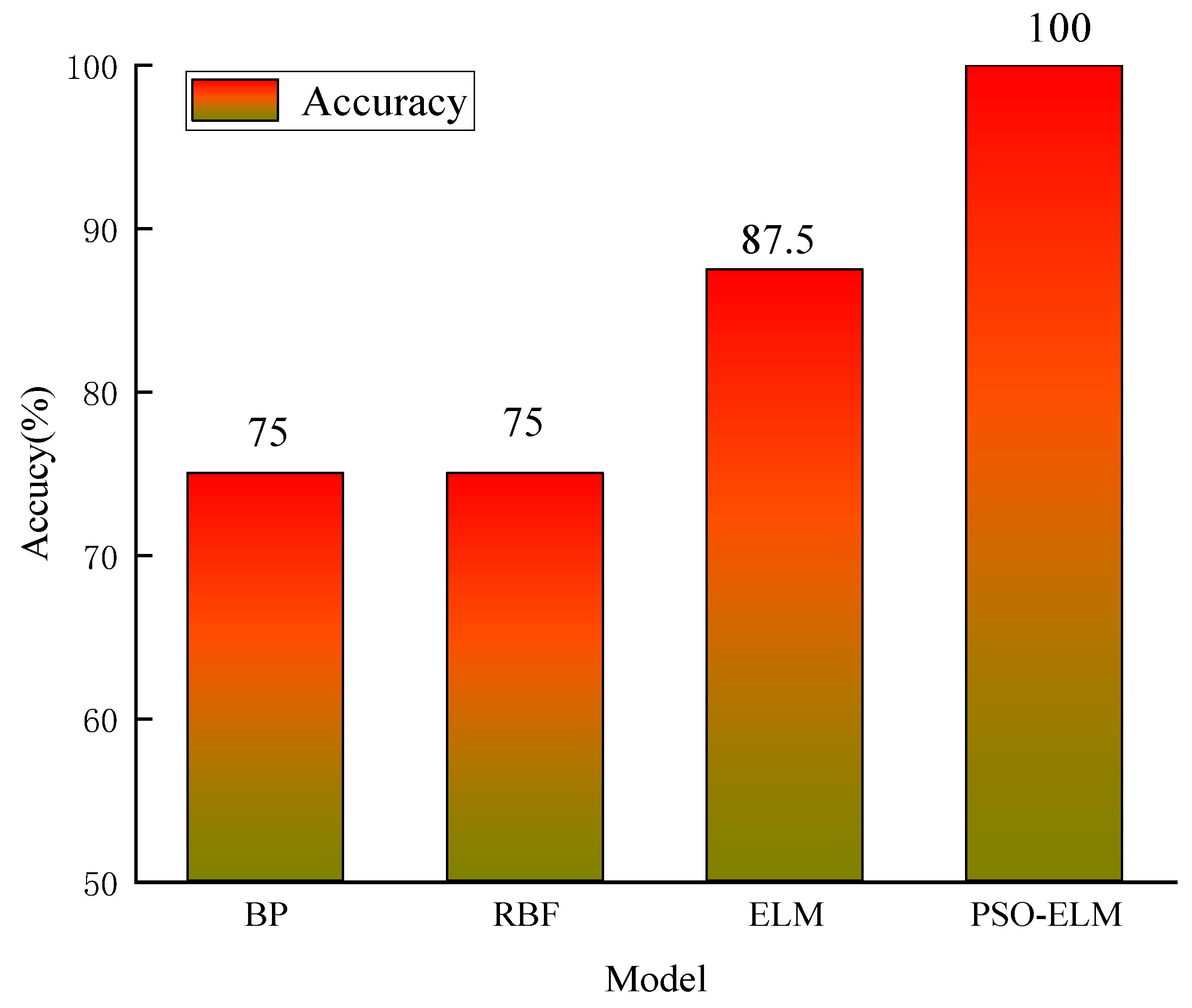
- Through the precision analysis and comparison between the prediction results of the BP neural network, radial basis function, and ELM, the research findings indicated that the prediction accuracy of the PSO–ELM model on the test set was as high as 100%, and the prediction accuracy was far better than the other three models.
- In summary, the rock burst PCA–PSO–ELM prediction model had the advantages for good prediction performance, fast learning speed, firm generalization ability, and satisfied robustness, which provided an idea for the early warning research of rock burst disasters and exhibited favorable engineering significance.
- It is worth noting that rock bursts are not only affected by the conditions of geology and mining technology, but also influenced by the hidden factors of Class II mining technology and so on during the prediction process of rock burst, such as the progress degree of the working face or the expansion and repair of roadway walls, prompting the risk rank assessment of rock bursts to become a difficult subject. Consequently, the investigation on intelligent early warning for rock bursts requires further research and discussion.
Author Contributions
Funding
Institutional Review Board Statement
Informed Consent Statement
Data Availability Statement
Conflicts of Interest
References
- Keneti, A.; Sainsbury, B.-A. Review of published rockburst events and their contributing factors. Eng. Geol. 2018, 246, 361–373. [Google Scholar] [CrossRef]
- Lv, P.; Qiu, L. Study on classification prediction of mine Rock burst based on PSO-LSSVM. Min. Saf. Environ. Prot. 2021, 48, 120–125. [Google Scholar]
- Xu, G.; Li, K.; Li, M.; Qin, Q.; Yue, R. Rockburst Intensity Level Prediction Method Based on FA-SSA-PNN Model. Energies 2022, 15, 5016. [Google Scholar] [CrossRef]
- Wu, M.; Ye, Y.; Wang, Q.; Hu, N. Development of Rockburst Research: A Comprehensive Review. Appl. Sci. 2022, 12, 974. [Google Scholar] [CrossRef]
- Wang, J.; Zhou, Z.; Li, K.; Wang, H.; Li, X. A risk grade evaluation model of Rock burst based on R-factor analysis and probabilistic neural network. Vib. Shock 2019, 38, 192–203. [Google Scholar]
- Waqar, M.F.; Guo, S.; Qi, S. A Comprehensive Review of Mechanisms, Predictive Techniques, and Control Strategies of Rockburst. Appl. Sci. 2023, 13, 3950. [Google Scholar] [CrossRef]
- Pan, Y.; Xu, L. Experimental study on predicting Rock burst with cuttings temperature method. J. Geotech. Eng. 2012, 34, 2228–2232. [Google Scholar]
- Feng, G.-L.; Chen, B.-R.; Xiao, Y.-X.; Jiang, Q.; Li, P.-X.; Zheng, H.; Zhang, W. Microseismic characteristics of rockburst development in deep TBM tunnels with alternating soft-hard strata and application to rockburst warning: A case study of the Neelum-Jhelum hydropower project. Tunn. Undergr. Space Technol. 2022, 122, 104398. [Google Scholar] [CrossRef]
- Feng, G.-L.; Feng, X.-T.; Chen, B.-R.; Xiao, Y.-X.; Yu, Y. A Microseismic Method for Dynamic Warning of Rockburst Development Processes in Tunnels. Rock Mech. Rock Eng. 2015, 48, 2061–2076. [Google Scholar] [CrossRef]
- Zhang, Z.-Z.; Gao, F.; Shang, X.-J. Rock burst proneness prediction by acoustic emission test during rock deformation. J. Cent. South Univ. 2014, 21, 373–380. [Google Scholar] [CrossRef]
- Zhang, H.; Chen, Q.; Wang, X.; Zhao, K.; Zeng, Q. Acoustic Emission Parameter Characterization of Damage Process of the Limestone with Different Rockburst Tendencies. Minerals 2022, 12, 1423. [Google Scholar] [CrossRef]
- Zhao, T.; Yin, Y.; Xiao, F.; Tan, Y.; Zou, J. Rockburst Disaster Prediction of Isolated Coal Pillar by Electromagnetic Radiation Based on Frictional Effect. Sci. World J. 2014, 2014, 814050. [Google Scholar] [CrossRef] [Green Version]
- Mu, H.; Song, D.; He, X.; Li, Z.; Su, D.; Xue, Y. Regional local integrated rockburst monitoring and early warning for multi-seam mining. J. Geophys. Eng. 2021, 18, 725–739. [Google Scholar] [CrossRef]
- Li, B.; Liu, Y. Random forest model and its application for Rock burst hazard grade identification. Technol. Her. 2015, 33, 57–62. [Google Scholar]
- Zhu, W.; Ren, M.; Dai, F.; Zhang, P.; Wang, L.; Liu, H.; Jia, H.; Wang, X. A method for predicting and warning mining disasters by combining on-site monitoring and numerical simulation. Met. Mines 2020, 151–162. [Google Scholar]
- Vacek, J.; Choholousova, J. Rock burst mechanics: Insight from physical and mathematical modelling. Acta Polytech. Czech Tech. Univ. Prague 2008, 48, 38–44. [Google Scholar] [CrossRef] [PubMed]
- Chen, G.; He, M.; Fan, F. Rock burst Analysis Using DDA Numerical Simulation. Int. J. Geomech. 2018, 18, 04018001. [Google Scholar] [CrossRef]
- Wang, H.; Nie, L.; Xu, Y.; Lv, Y.; He, Y.; Du, C.; Zhang, T.; Wang, Y. Comprehensive Prediction and Discriminant Model for Rockburst Intensity Based on Improved Variable Fuzzy Sets Approach. Appl. Sci. 2019, 9, 3173. [Google Scholar] [CrossRef] [Green Version]
- Gu, X.-B.; Wu, Q.-H.; Ma, Y. Risk Assessment of the ockburst Intensity in a Hydraulic Tunnel Using an Intuitionistic Fuzzy Sets-TOPSIS Model. Adv. Mater. Sci. Eng. 2022, 2022, 4774978. [Google Scholar] [CrossRef]
- Xue, Y.; Li, Z.; Li, S.; Qiu, D.; Tao, Y.; Wang, L.; Yang, W.; Zhang, K. Prediction of rock burst in underground caverns based on rough set and extensible comprehensive evaluation. Bull. Eng. Geol. Environ. 2019, 78, 417–429. [Google Scholar] [CrossRef]
- Xue, Y.; Bai, C.; Kong, F.; Qiu, D.; Li, L.; Su, M.; Zhao, Y. A two-step comprehensive evaluation model for rockburst prediction based on multiple empirical criteria. Eng. Geol. 2020, 268, 105515. [Google Scholar] [CrossRef]
- Zhou, K.-P.; Lin, Y.; Deng, H.-W.; Li, J.-L.; Liu, C.-J. Prediction of rock burst classification using cloud model with entropy weight. Trans. Nonferrous Met. Soc. China 2016, 26, 1995–2002. [Google Scholar] [CrossRef]
- Liu, R.; Ye, Y.; Hu, N.; Chen, H.; Wang, X. Classified prediction model of rockburst using rough sets-normal cloud. Neural Comput. Appl. 2019, 31, 8185–8193. [Google Scholar] [CrossRef]
- Ji, M.; Guo, H.-J.; Zhang, Y.-D.; Li, T.; Gao, L.-S. Hierarchic Analysis Method to Evaluate Rock burst Risk. Math. Probl. Eng. 2015, 2015, 184398. [Google Scholar] [CrossRef] [Green Version]
- Zhu, Z.; Zhang, H.; Han, J.; Lv, Y. A Risk Assessment Method for Rockburst Based on Geodynamic Environment. Shock. Vib. 2018, 2018, 2586842. [Google Scholar] [CrossRef]
- Zheng, Y.; Zhong, H.; Fang, Y.; Zhang, W.; Liu, K.; Fang, J. Rockburst Prediction Model Based on Entropy Weight Integrated with Grey Relational BP Neural Network. Adv. Civ. Eng. 2019, 2019, 3453614. [Google Scholar] [CrossRef]
- Zhang, Z.P.; Xu, A.; Liu, G. Set pair analysis and evaluation model of Rock burst risk. J. China Univ. Min. Technol. 2011, 40, 379–384. [Google Scholar]
- Zhou, J.; Li, X.; Mitri, H.S. Evaluation method of rockburst: State-of-the-art literature review. Tunn. Undergr. Space Technol. 2018, 81, 632–659. [Google Scholar] [CrossRef]
- Zhang, K.; Zhu, J.; He, M.; Jiang, Y.; Zhu, C.; Li, D.; Kang, L.; Sun, J.; Chen, Z.; Wang, X.; et al. Research on Intelligent Comprehensive Evaluation of Coal Seam Impact Risk Based on BP Neural Network Model. Energies 2022, 15, 3292. [Google Scholar] [CrossRef]
- Zhou, J.; Shi, X.-z.; Huang, R.-d.; Qiu, X.-y.; Chen, C. Feasibility of stochastic gradient boosting approach for predicting rockburst damage in burst-prone mines. Trans. Nonferrous Met. Soc. China 2016, 26, 1938–1945. [Google Scholar] [CrossRef]
- Zhao, H.; Chen, B. Data-Driven Model for Rockburst Prediction. Math. Probl. Eng. 2020, 2020, 5735496. [Google Scholar] [CrossRef]
- Ma, L.; Cai, J.; Dai, X.; Jia, R. Research on Rockburst Risk Level Prediction Method Based on LightGBM-TCN-RF. Appl. Sci. 2022, 12, 8226. [Google Scholar] [CrossRef]
- Ji, B.; Xie, F.; Wang, X.; He, S.; Song, D. Investigate Contribution of Multi-Microseismic Data to Rockburst Risk Prediction Using Support Vector Machine with Genetic Algorithm. IEEE Access 2020, 8, 58817–58828. [Google Scholar] [CrossRef]
- Yuan, H.; Cao, Z.; Xiong, L.; Li, H.; Wang, Y. A Machine Learning Method for Engineering Risk Identification of Goaf. Water 2022, 14, 4075. [Google Scholar] [CrossRef]
- Wang, D.; Tan, D.; Liu, L. Particle swarm optimization algorithm: An overview. Soft Comput. 2018, 22, 387–408. [Google Scholar] [CrossRef]
- Zhang, Y.; Wang, S.; Ji, G. A Comprehensive Survey on Particle Swarm Optimization Algorithm and Its Applications. Math. Probl. Eng. 2015, 2015, 931256. [Google Scholar] [CrossRef] [Green Version]
- Ding, S.; Zhao, H.; Zhang, Y.; Xu, X.; Nie, R. Extreme learning machine: Algorithm, theory and applications. Artif. Intell. Rev. 2015, 44, 103–115. [Google Scholar] [CrossRef]
- Huang, G.; Huang, G.-B.; Song, S.; You, K. Trends in extreme learning machines: A review. Neural Netw. 2015, 61, 32–48. [Google Scholar] [CrossRef]
- Huang, G.; Song, S.; Gupta, J.N.D.; Wu, C. Semi-Supervised and Unsupervised Extreme Learning Machines. IEEE Trans. Cybern. 2014, 44, 2405–2417. [Google Scholar] [CrossRef]
- Dai, G. Research on Nonlinear Dynamic Characteristics of Rock and Rock Burst. Ph.D. Thesis, Chongqing University, Chongqing, China, 2002. [Google Scholar]


| Assignment | Qualitative Index of Rock Bursts | |||||
|---|---|---|---|---|---|---|
| X4 | X5 | X6 | X8 | X9 | X10 | |
| 0 | Simple | Unchanged | Unchanged | No support or poor support | No pressure relief measures | None |
| 1 | Average | Minor change | Minor change | Average | Average pressure relief effect | Less |
| 2 | Relatively complex | Relatively large changes | Relatively large changes | Relatively good | Relatively good pressure relief effect | Many |
| 3 | Complex | Severe change | Severe change | Good | Good pressure relief effect | |
| Sample | X1 | X2 | X3 | X4 | X5 | X6 | X7 | X8 | X9 | X10 | Impact Level |
|---|---|---|---|---|---|---|---|---|---|---|---|
| 1 | 1.3 | 29 | 530 | 0 | 0 | 0 | 0.07 | 3 | 3 | 0 | Ι |
| 2 | 1.2 | 25 | 542 | 0 | 0 | 0 | 0.24 | 3 | 3 | 0 | Ι |
| 3 | 1.4 | 44 | 560 | 0 | 0 | 0 | 0.09 | 3 | 3 | 0 | Ι |
| 4 | 3 | 24 | 573 | 0 | 0 | 1 | 0.36 | 2 | 3 | 0 | Ι |
| 5 | 0.8 | 34 | 553 | 1 | 0 | 0 | 0.15 | 0 | 2 | 1 | Ⅱ |
| 6 | 1.2 | 40 | 490 | 0 | 0 | 0 | 0.2 | 2 | 0 | 1 | Ⅱ |
| 7 | 1.4 | 35 | 480 | 0 | 0 | 1 | 0.36 | 2 | 0 | 1 | Ⅱ |
| 8 | 1.2 | 27 | 490 | 0 | 0 | 0 | 0.64 | 2 | 2 | 1 | Ⅱ |
| 9 | 2.6 | 48 | 752 | 2 | 0 | 2 | 0.48 | 1 | 1 | 1 | Ⅲ |
| 10 | 2.8 | 52 | 733 | 0 | 1 | 1 | 0.54 | 2 | 2 | 1 | Ⅲ |
| 11 | 3 | 78 | 560 | 1 | 3 | 2 | 1.14 | 2 | 3 | 1 | Ⅲ |
| 12 | 6 | 30 | 465 | 1 | 1 | 3 | 1.3 | 1 | 0 | 2 | Ⅲ |
| 13 | 1.5 | 65 | 570 | 1 | 3 | 1 | 0.28 | 1 | 2 | 2 | Ⅲ |
| 14 | 3 | 35 | 612 | 2 | 0 | 2 | 0.56 | 2 | 0 | 2 | Ⅲ |
| 15 | 2 | 35 | 614 | 1 | 0 | 2 | 0.56 | 1 | 0 | 2 | Ⅲ |
| 16 | 3 | 55 | 855 | 3 | 2 | 3 | 0.075 | 1 | 1 | 2 | Ⅳ |
| 17 | 4 | 52 | 675 | 3 | 2 | 3 | 1.88 | 0 | 0 | 2 | Ⅳ |
| 18 | 1.3 | 73 | 486 | 3 | 3 | 3 | 0.43 | 1 | 0 | 2 | Ⅳ |
| 19 | 2.1 | 67 | 498 | 3 | 3 | 3 | 1.89 | 0 | 0 | 2 | Ⅳ |
| 20 | 2.5 | 65 | 450 | 3 | 2 | 3 | 0.67 | 1 | 1 | 2 | Ⅳ |
| 21 | 1.7 | 60 | 314 | 3 | 3 | 1 | 1.3 | 0 | 0 | 2 | Ⅳ |
| 22 | 1.1 | 47 | 485 | 3 | 3 | 3 | 0.43 | 1 | 0 | 2 | Ⅳ |
| 23 | 1.8 | 54 | 238 | 3 | 1 | 3 | 1 | 0 | 0 | 2 | Ⅳ |
| 24 | 1.6 | 35 | 583 | 2 | 0 | 3 | 1.5 | 3 | 3 | 1 | Ⅱ |
| 25 | 1.5 | 35 | 530 | 0 | 0 | 0 | 0.56 | 3 | 3 | 0 | Ⅰ |
| 26 | 1.6 | 62 | 307 | 3 | 2 | 2 | 1 | 0 | 0 | 2 | Ⅳ |
| 27 | 1.9 | 59 | 542 | 1 | 2 | 3 | 0.25 | 0 | 0 | 1 | Ⅲ |
| Sample | X1 | X2 | X3 | X4 | X5 | X6 | X7 | X8 | X9 | X10 | Impact Level |
|---|---|---|---|---|---|---|---|---|---|---|---|
| 1 | 1.8 | 62 | 283 | 3 | 2 | 3 | 1 | 0 | 0 | 2 | Ⅳ |
| 2 | 1.3 | 44 | 570 | 0 | 0 | 0 | 0.66 | 3 | 3 | 0 | Ι |
| 3 | 2.2 | 54 | 290 | 3 | 2 | 2 | 1 | 0 | 0 | 2 | Ⅳ |
| 4 | 3 | 34 | 475 | 2 | 2 | 1 | 0.42 | 0 | 0 | 2 | Ⅲ |
| 5 | 3.2 | 42 | 574 | 3 | 0 | 0 | 0.29 | 0 | 0 | 2 | Ⅲ |
| 6 | 1.8 | 62 | 283 | 3 | 2 | 3 | 1 | 0 | 0 | 2 | Ⅳ |
| 7 | 1.3 | 44 | 656 | 2 | 1 | 3 | 0.24 | 1 | 1 | 2 | Ⅲ |
| 8 | 1.2 | 40 | 553 | 2 | 2 | 2 | 0.49 | 1 | 2 | 2 | Ⅲ |
| Fitness Quantity of KMO Sampling | 0.753 | |
|---|---|---|
| Approximate chi square | 302.168 | |
| Bartlett sphericity test | Degree of freedom | 45 |
| Significance | 0.000 |
| Sample | Principal Component | Impact Level | |||||
|---|---|---|---|---|---|---|---|
| Y1 | Y2 | Y3 | Y4 | Y5 | Y6 | ||
| 1 | −4.13 | −0.52 | 0.22 | 0.38 | 0.23 | 0.13 | Ⅰ |
| 2 | −4.15 | −0.38 | 0.17 | 0.55 | 0.38 | −0.09 | Ⅰ |
| 3 | −3.84 | −0.73 | 0.80 | 0.24 | 0.05 | 0.23 | Ⅰ |
| 4 | −3.22 | 0.99 | 0.37 | 0.73 | −0.23 | −0.2 | Ⅰ |
| 5 | −1.85 | −0.83 | −1.1 | −0.77 | −0.59 | −1.5 | Ⅱ |
| 6 | −2.12 | −0.56 | −1.35 | −0.17 | −0.30 | 0.7 | Ⅱ |
| 7 | −1.79 | −0.13 | −1.32 | 0.11 | 0.2 | 0.83 | Ⅱ |
| 8 | −2.67 | −0.29 | −0.79 | 0.71 | 0 | −0.35 | Ⅱ |
| 9 | −0.49 | 1.15 | 0.43 | −1.07 | 0.33 | −0.63 | Ⅲ |
| 10 | −1.63 | 0.74 | 1.42 | −0.3 | −0.68 | 0.17 | Ⅲ |
| 11 | 0.31 | −0.61 | 3.04 | 1.19 | −0.63 | 0.38 | Ⅲ |
| 12 | 1.39 | 3.2 | −0.65 | 1.65 | −0.81 | 0.99 | Ⅲ |
| 13 | 0.27 | −1.48 | 1.15 | −0.82 | −1.12 | 0.24 | Ⅲ |
| 14 | −0.06 | 1.57 | −0.78 | −0.53 | 0.64 | 0.56 | Ⅲ |
| 15 | −0.17 | 0.94 | −1.15 | −0.74 | 0.35 | 0.08 | Ⅲ |
| 16 | 1.17 | 1.16 | 1.43 | −2.5 | 0.17 | 0.03 | Ⅳ |
| 17 | 2.96 | 1.96 | 0.66 | 0.65 | −0.06 | −1.04 | Ⅳ |
| 18 | 2.34 | −1.54 | 0.55 | −0.89 | 0.44 | 0.86 | Ⅳ |
| 19 | 3.44 | −0.4 | 0.62 | 1.04 | 0.26 | −0.73 | Ⅳ |
| 20 | 1.96 | −0.5 | 0.51 | −0.05 | 0.36 | 0.47 | Ⅳ |
| 21 | 2.48 | −1.62 | −0.7 | 1.06 | −0.70 | −0.52 | Ⅳ |
| 22 | 1.80 | −1.02 | −0.29 | −0.84 | 0.80 | 0.55 | Ⅳ |
| 23 | 2.34 | −0.94 | −1.54 | 0.95 | 0.67 | 0.02 | Ⅳ |
| 24 | −1.14 | 0.75 | 1.15 | 1.42 | 2.49 | −0.62 | Ⅱ |
| 25 | −3.74 | −0.37 | 0.56 | 1.06 | 0.25 | −0.14 | Ⅰ |
| 26 | 2.39 | −1.44 | −0.92 | 0.62 | −0.05 | −0.18 | Ⅳ |
| 27 | 0.87 | −0.54 | 0.03 | −0.78 | −0.37 | 0.54 | Ⅲ |
| Sample | Principal Component | Impact Level | |||||
|---|---|---|---|---|---|---|---|
| Y1 | Y2 | Y3 | Y4 | Y5 | Y6 | ||
| 1 | 2.74 | −1.24 | −0.83 | 0.73 | 0.34 | 0.16 | Ⅳ |
| 2 | −3.57 | −0.55 | 0.98 | 0.95 | 0.28 | −0.25 | Ⅰ |
| 3 | 2.33 | −0.94 | −1.16 | 0.83 | −0.22 | −0.1 | Ⅳ |
| 4 | 0.94 | 0.31 | −1.36 | −0.38 | −1.24 | −0.08 | Ⅲ |
| 5 | 0.42 | 0.81 | −1.59 | −1.1 | −1.11 | −0.9 | Ⅲ |
| 6 | 2.74 | −1.24 | −0.83 | 0.73 | 0.34 | 0.16 | Ⅳ |
| 7 | 0.37 | 0.09 | −0.03 | −1.56 | 0.96 | 0.01 | Ⅲ |
| 8 | 0.21 | −0.64 | 0.15 | −0.61 | 0.37 | −0.4 | Ⅲ |
| Test Sample | Actual Grade | BP | RBF | ELM | PSO–ELM |
|---|---|---|---|---|---|
| 1 | Ⅳ | Ⅳ | Ⅳ | Ⅳ | Ⅳ |
| 2 | Ⅰ | Ⅰ | Ⅰ | Ⅰ | Ⅰ |
| 3 | Ⅳ | Ⅳ | Ⅳ | Ⅳ | Ⅳ |
| 4 | Ⅲ | Ⅲ | Ⅲ | Ⅲ | Ⅲ |
| 5 | Ⅲ | Ⅳ | Ⅳ | Ⅲ | Ⅲ |
| 6 | Ⅳ | Ⅳ | Ⅳ | Ⅳ | Ⅳ |
| 7 | Ⅲ | Ⅲ | Ⅲ | Ⅳ | Ⅲ |
| 8 | Ⅲ | Ⅳ | Ⅱ | Ⅲ | Ⅲ |
Disclaimer/Publisher’s Note: The statements, opinions and data contained in all publications are solely those of the individual author(s) and contributor(s) and not of MDPI and/or the editor(s). MDPI and/or the editor(s) disclaim responsibility for any injury to people or property resulting from any ideas, methods, instructions or products referred to in the content. |
© 2023 by the authors. Licensee MDPI, Basel, Switzerland. This article is an open access article distributed under the terms and conditions of the Creative Commons Attribution (CC BY) license (https://creativecommons.org/licenses/by/4.0/).
Share and Cite
Yuan, H.; Ji, S.; Liu, G.; Xiong, L.; Li, H.; Cao, Z.; Xia, Z. Investigation on Intelligent Early Warning of Rock Burst Disasters Using the PCA-PSO-ELM Model. Appl. Sci. 2023, 13, 8796. https://doi.org/10.3390/app13158796
Yuan H, Ji S, Liu G, Xiong L, Li H, Cao Z, Xia Z. Investigation on Intelligent Early Warning of Rock Burst Disasters Using the PCA-PSO-ELM Model. Applied Sciences. 2023; 13(15):8796. https://doi.org/10.3390/app13158796
Chicago/Turabian StyleYuan, Haiping, Shuaijie Ji, Gaoliang Liu, Lijun Xiong, Hengzhe Li, Zhanhua Cao, and Zijin Xia. 2023. "Investigation on Intelligent Early Warning of Rock Burst Disasters Using the PCA-PSO-ELM Model" Applied Sciences 13, no. 15: 8796. https://doi.org/10.3390/app13158796