An Explanation of the LSTM Model Used for DDoS Attacks Classification

Abstract

With the rise of DDoS attacks, several machine learning-based attack detection models have been used to mitigate malicious behavioral attacks. Understanding how machine learning models work is not trivial. This is particularly true for complex and nonlinear models, such as deep learning models that have high accuracy. The struggle to explain these models creates a tension between accuracy and explanation. Recently, different methods have been used to explain deep learning models and address ambiguity issues. In this paper, we utilize the LSTM model to classify DDoS attacks. We then investigate the explanation of LSTM using LIME, SHAP, Anchor, and LORE methods. Predictions of 17 DDoS attacks are explained by these methods, where common explanations are obtained for each class. We also use the output of the explanation methods to extract intrinsic features needed to differentiate DDoS attacks. Our results demonstrate 51 intrinsic features to classify attacks. We finally compare the explanation methods and evaluate them using descriptive accuracy (DA) and descriptive sparsity (DS) metrics. The comparison and evaluation show that the explanation methods can explain the classification of DDoS attacks by capturing either the dominant contribution of input features in the prediction of the classifier or a set of features with high relevance.

1. Introduction

Recently, the risk of cyberattacks has increased because of vulnerabilities in some internet-connected devices that often make them easy targets [1]. DDoS attacks are particularly challenging to combat compared to other types of malicious cyberattacks. It has proven difficult to detect these types of attacks because of their ability to mask themselves as legitimate traffic.

Denial of Service (DoS) attacks are among the most popular and threatening attacks on network security [2]. This threat is represented in violating the availability of network services by denying authorized users from accessing the targeted services. Unlike DoS attacks that are launched from a single source, DDoS attacks are launched in a distributed manner from several sources. Attackers perform a DDoS attack in order to overwhelm the target with a relentless flood of traffic, which results in consuming the computational power, as well as the network capacity of network links [3].

The first DDoS attack was performed in August 1999 on the University of Minnesota computer network [4]. The attacker was able to shut down the network computers for about two days. In February 2000, famous websites such as eBay, Yahoo, Buy, and Amazon were attacked by a high-profile DDoS attack [4]. After that, DDoS attacks continued growing in frequency, and today they employ IoT devices and adopt new complicated methods to be widespread [2,5,6,7,8]. According to Cloudflare’s DDoS Threat Report Q3 of 2022 [9], DDoS attacks, in general, increased compared to the previous year. Application layer attacks (HTTP DDoS and Ransom DDoS) increased by 111% and 67%, respectively, in 2022 compared to the previous year. Network layer attacks (Layers 3 and 4 DDoS) increased by 97% in 2022 compared to the previous year and 24% in Q3 compared to the same quartile of the previous year.

Since the advent of DDoS attacks, the research community has tackled this threat through several detection techniques, including the following: trace back scheme, traffic filtering autonomous system, signature-based detection, and anomaly-based detection [10]. The tracing scheme relies on finding the locations of attack sources, while an autonomous traffic filtering system utilizes traffic filtering to isolate traffic that is not originating or destined for the network. The signature-based detection scheme builds its own database from known malicious threats and compares the new traffic to that database to identify malicious activities, whereas the anomaly-based detection scheme monitors the network behavior to distinguish malicious activities from the normal traffic based on a training process. Machine learning (ML) techniques belong to the last-mentioned category.

ML can be used to detect intrusions in network traffic as one of the most effective detection techniques [11]. In particular, deep learning (DL) has exhibited excellent performance in recent years. As real data are nonlinear, complex, and highly dimensional, the construction of DL models has several hidden neurons, and each neuron has a nonlinear function. The complex construction of DL models makes them better at understanding certain complex and nonlinear data in the target domain.

Although DL models are a powerful tool for modeling data and improving performance, they, unfortunately, can complicate the model explanation process. Thus, DL models are considered to be complex black-box models. The tradeoff between performance and explanation is the main issue in black-box models. Though DL models exhibit high performance, they are difficult to explain. To overcome this issue, explanation methods have been expanded to interpret DL models and explain their predictions.

The most prominent explanation methods are local, model-agnostic methods that focus on explaining individual outputs of a given black-box model, including LIME [12], SHAP [13], Anchor [14], and LORE [15] explanation methods. These methods assess the contribution of individual features in a specific prediction by generating perturbation samples of a given data instance and monitoring the effect of these perturbation samples on DL model output.

In this paper, we utilize Recurrent Neural Networks (RNNs) for DDoS attack classification. RNNs are strong and robust neural networks that are among the most effective algorithms as they have internal memory. They utilize their internal memory to recall important characteristics of the input they receive. For this reason, RNNs are the preferred models for dealing with sequential data such as time series [16,17,18,19]. The LSTM network is a modified version of the recurrent neural network. LSTM is well suited for processing, classifying, and predicting time series data with unknown time spans.

We then investigate the explanation of the LSTM predictions using LIME, SHAP, Anchor, and LORE explanation methods. We adopt the above explanation methods to interpret LSTM classification model predictions for two main reasons. First, these explanation methods have local interpretability, meaning they concentrate on interpreting individual predictions for a particular black-box classifier. This property is appropriate to interpret a decision taken and why a certain instance is considered an attack. Second, unlike the other explanation approaches that are designed to interpret specific models, the above four explanation methods are model-agnostic approaches that can be utilized by any classification model.

In this paper, we investigate the use of the long short-term memory (LSTM) model in classifying DDoS attacks while focusing on the explanation of the DL model’s predictions using LIME, SHAP, Anchor, and LORE methods. We can summarize our main contributions as follows:

• Assess the LSTM performance in detecting different classes of DDoS attacks by utilizing commonly used and publicly available CIC datasets;
• Investigate the explanation of LSTM predictions on DDoS attacks in CIC datasets using four different explanation methods;
• Utilize the output of explanation methods to demonstrate intrinsic classification features and improve LSTM classification performance, particularly on the CICDDoS2019 dataset;
• Compare and evaluate the explanation methods in the domain of DDoS attack classification using two evaluation metrics.

The remainder of the paper is organized as follows: in Section 2, we present the background of three explanation methods that we implement in this work. Section 3 shows recent work on the classification of DDoS attacks using the DL models and explanation methods that are used to interpret the DL models. Section 4 describes the methodology we adopt to classify the DDoS attacks using LSTM classifier and the explanation methods to interpret the LSTM predictions. This section, in particular, includes dataset preprocessing, classification model design, and the explanation methods used. The classification of the DDoS attacks using the LSTM model, the evaluation of the predictions, and their explanation are presented in Section 5. We show our conclusions and future work in Section 6.

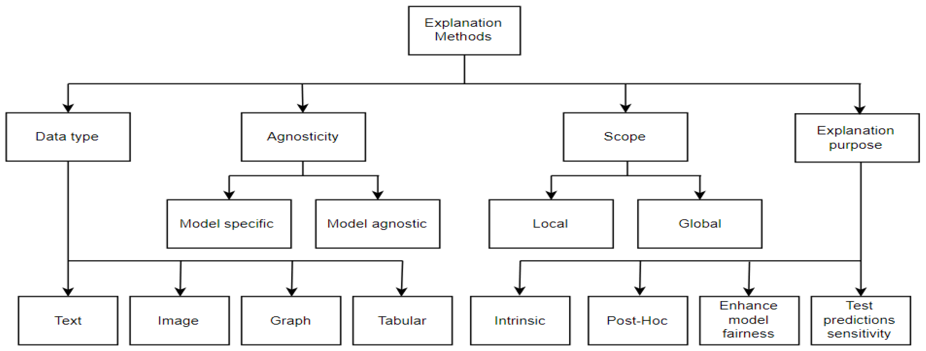
2. Explanation Methods

Linardatos et al. [20] summarized the various aspects through which explanation methods can be categorized. Figure 1 visualizes these aspects: data type, agnosticity, scope, and explanation purpose.

Depending on the data that needs to be explained, explanation methods can be graph-based, image-based, text-based, and tabular-based, while the agnosticity indicates if the explanation method is applicable to explain any type of ML model or if it can explain only a specific type. Some of the explanation methods are local explanations because they are used to explain individual predictions instead of the whole model. The explanation methods can also be classified regarding the purpose of explanation into intrinsic, post hoc, enhanced model fairness, and test predictions sensitivity. Intrinsic-based explanation methods create interpretable models instead of complex models, while post hoc-based methods attempt to interpret complex models instead of using interpretable models. Although fairness is a surprisingly new field of ML explanation [20], the development made in the closing few years was not trivial. Several explanation methods have been produced to improve the fairness of ML models and guarantee the fair allocation of resources.

One of the purposes of the explanation methods is to test the sensitivity of model prediction. Several explanation methods try to evaluate and challenge ML models to support the trustworthiness and reliability of predictions of these models. These methods employ a composition used to analyze the sensitivity, where models are examined in terms of how sensitive their predictions are regarding the fine fluctuations in the corresponding inputs.

The taxonomy in Figure 1 focuses on the purpose for which these methods were created and the approaches they use to accomplish that purpose. In accordance with the taxonomy, four main categories for explanation methods can be distinguished [20]: methods to interpret complex black-box models, methods to generate white-box models, methods to ensure fairness and restrict the existence of discrimination, and, finally, methods to analyze the model prediction sensitivity. According to [20], methods to interpret complex black-box models can be categorized into methods to interpret DL models and methods to interpret any black-box models. Methods to analyze the model prediction sensitivity can also be classified as traditional analysis methods and adversarial example-based analysis methods. The LIME, SHAP, Anchor, and LORE explanation methods, the models we employ in our work, belong to the methods to explain any black-box models.

Ribeiro et al. [12] proposed the LIME explanation framework that can interpret the outputs of any classification model in an explainable and trusted way. This method relies on learning an explainable model in a local manner around the model output. They proposed an extension framework called (SP-LIME) to interpret models globally by providing representative explanations of individual outputs in a non-redundant manner. The proposed frameworks were evaluated with simulated and human subjects by measuring the impact of explanations on trust and associated tasks. The authors also showed how understanding the predictions of a neural network on images helps practitioners know when and why they should not trust a model.

Lundberg and Lee [13] proposed the SHAP method to explain the ML model, where the importance of the input features is measured by the Shapley values. These values are inspired by the field of cooperative game theory, which aims to quantify each player’s contribution to the game. They arise in situations where the number of players (features of input data) collaborates to acquire a reward (prediction of ML model). The proposed approach was evaluated by applying kernel SHAP and Deep SHAP approximations on the CNN’s DL model used to classify digital images from the MNIST dataset.

In another work, Ribeiro et al. [14] introduced a model diagnostic system called Anchor. The Anchor model utilizes a strategy that is based on the perturbation technique to generate local explanations for the ML model outputs. Therefore, instead of the linear regression models implemented by the LIME method, the Anchor explanations are presented as IF–THEN rules that are easy to understand. Anchors adopt the concept of coverage to state exactly which other and possibly unseen instances they apply to. Anchors are determined by methods of an exploration or multi-armed bandit problem, which has its roots in the discipline of reinforcement learning. Several ML models, Logistic Regression (LR), Gradient-Boosted trees (GB), and Multilayer Perceptron (MLP), were explained in this paper to show the flexibility of the Anchor method.

Guidotti et al. [15] proposed an agnostic method called LORE which provides interpretable and faithful explanations of the ML models. Firstly, a genetic algorithm is used to generate a synthetic neighborhood around the intended instance to allow LORE to learn a local explainable predictor. Then, LORE exploits the concept of the local explainable predictor to derive significant explanations, including decision rules that explain the causes behind the decision and counterfactual rules. These rules present the fluctuations in the features of inputs that lead to a different prediction. SVM, RF, and MLP ML models were explained, in this work, using LORE on three datasets (adult, German, and compass).

2.1. LIME

LIME stands for Local Interpretable Model-agnostic Explanations. It was developed by Ribeiro et al. [12]. This method is local and model-agnostic because it can explain local individual prediction for any kind of ML model.

The goal of the explanation is to comprehend why the black-box model made a certain prediction. LIME explains the model prediction locally by investigating what occurs to the prediction when the input data instance is varied (perturbed). To this end, LIME generates new samples that consist of perturbed instances, and the black box is used to find corresponding predictions of these new samples. LIME then trains a simple explainable model, which gains weight by the vicinity of the perturbed instances to the interesting instance. The simple explainable model can be chosen from the explainable model’s space; for instance, this model can be Least Absolute Shrinkage and Selection Operator (LASSO) [21]. LASSO uses $L_1$ regularization to avoid problem of overfitting in ML models and improve the prediction accuracy and interpretability. Mathematically, LIME explanation could be expressed as

$$\mathrm{E}\mathrm{x}\mathrm{p}\mathrm{l}\left(x\right)=\underset{g\in G}{\mathrm{argmin}}\mathcal{L}\left(f,g,{\pi }_x\right)+\mathsf{\Omega }\left(g\right),$$

(1)

where $g$ is the explainable model for instance $x$ that minimizes loss $\mathcal{L}$. $G$ is the group of available explainable models, for instance, all possible linear regression models. $\mathcal{L}$ estimates how the explanation is close to the prediction of the intended black-box model $f$. $\mathsf{\Omega }\left(g\right)$ is a penalty term to measure the complexity of explanation result. The vicinity measure, ${\pi }_x$, determines how the neighborhood we consider for the explanation around instance $x$ is large.

2.2. SHAP

Shapley Additive Explanation (SHAP) method was presented by Lundberg and Lee [13]. SHAP method is based on calculating the Shapley Values [22]. Shapley value represents the contribution of each feature of input instance x in making the prediction of black-box model.

The Shapley values are inspired by the cooperative game theory that aims to quantify the contribution of each player (the feature in our case) in the game where a number of players collaborate to acquire a reward (the prediction in our case). The reward is supposed to be paid equitably between the players based on their contributions; such a contribution is the Shapley value. Simply, a Shapley value is defined as the average marginal contribution of a feature in an instance for all possible coalitions. The marginal contribution of a given feature is the difference between the prediction that is generated when the feature is present with respect to the prediction that is generated when that feature is absent. This is carried out for each of the coalitions. The coalitions are all possible subsets that can be generated where the feature we are looking to calculate has its contribution present. The mean of marginal contribution is the Shapley value. For instance $x$ with $F$ features, the Shapley value $\phi$ of the feature $i$ could be calculated as

$${\phi }_i\left(f,x\right)=\sum _{S\subseteq \left\{1,..,F\right\}\backslash \left\{i\right\}}\frac{\left|S\right|!\left(F-\left|S\right|-1\right)!}{F!}\left[f_x\left(S\cup \left\{i\right\}\right)-f_x\left(S\right)\right],$$

(2)

As a real dataset usually has a large number of features, this causes it to be computationally complicated to figure out the Shapley values for each feature individually in the interested instance. To avoid this, Lundberg and Lee introduced Kernel SHAP to approximate the SHAP method. Kernel SHAP is a method for calculating Shapley values with a smaller number of coalition instances. It relies on a weighted linear regression with the Shapley values as the solution coefficients.

2.3. Anchor

The Anchor method was developed by Ribeiro et al. [14], and they compared it to their previous work on LIME. The Anchor method is also called scoped rules method because it is based on IF–THEN rules, and these rules can be used more than one time since they are scoped. Anchors use the concept of coverage to specify which other, presumably unobserved, situations they apply to. Anchors minimize the number of model calls and combine reinforcement learning techniques [23] with a graph search algorithm [24] or recover from local optimum.

If we suppose that $D$ is the perturbation generated using the LIME method near the interested instance, the Anchor method constrains the perturbation space $D$ with Anchor $A$ that contains set of predicates ($D\left(.|A\right)$). For the input instance $x$, $A\left(x\right)$ returns $1$ if all its rules are true. Therefore, $A$ is an Anchor if $A\left(x\right)=1$, and $A$ represents a sufficient condition for the prediction $f\left(x\right)$, with high probability. This means that for a perturbed instance $x^{\prime }$ from $D\left(\frac{x^{\prime }}{A}\right)$, $f\left(x\right)=f\left(x^{\prime }\right)$. Formally $A$ is an Anchor if

$${\mathbb{E}}_{D\left(x^{\prime }|A\right)}\left[{\mathbb{1}}_{f\left(x\right)=f\left(x^{\prime }\right)}\right]\ge \tau , A\left(x\right)=1,$$

(3)

where $\tau$ is the desired level of precision. As the precision of the Anchor refers to the proportion of true predictions by the Anchor rules, we can use (3) to express the precision of $A$ that achieves $\mathrm{p}\mathrm{r}\mathrm{e}\mathrm{c}\left(A\right)\ge \tau$ as:

$$\mathrm{p}\mathrm{r}\mathrm{e}\mathrm{c}\left(A\right)={\mathbb{E}}_{D\left(x^{\prime }|A\right)}\left[{\mathbb{1}}_{f\left(x\right)=f\left(x^{\prime }\right)}\right],$$

(4)

For an arbitrary $D$ and black-box model $f$, directly computing this precision is impossible. Instead, a probabilistic definition is introduced where Anchors accept the precision constraint with a high probability:

$$P\left(\mathrm{p}\mathrm{r}\mathrm{e}\mathrm{c}\left(A\right)\ge \tau \right)\ge 1-\delta$$

(5)

The Anchor coverage is defined as the proportion of the input instances that are covered by the Anchor. Formally, the coverage of an Anchor can be expressed as the probability that it applies to instances from $D$, i.e., $\mathrm{c}\mathrm{o}\mathrm{v}\left(A\right)={\mathbb{E}}_{D\left(x^{\prime }\right)}\left[A\left(x^{\prime }\right)\right]$. Thus, the searching process for an Anchor $A$ is defined as combinatorial optimization problem:

$$\underset{\mathit{A} \mathrm{s}.\mathrm{t}. \mathit{P}\left(\mathrm{prec}\left(A\right)\ge \tau \right)\ge 1-\mathit{\delta }}{\max }\mathrm{c}\mathrm{o}\mathrm{v}\left(A\right)$$

(6)

The Anchor method utilizes a multi-armed bandit formulation algorithm [25]. This algorithm can randomly build the Anchors with the highest coverage and a particular threshold of precision.

2.4. LORE

LOcal Rule Explanation (LORE) method was introduced by Guidoti et al. [15]. This method is similar to the Anchor method in using rules to explain the decision of ML models. However, it differs from Anchor by generating perturbations of x by implementing a genetic algorithm (instead of linear regression) and training a decision tree (instead of linear regression) using two fitness functions.

LORE first uses a genetic algorithm to produce a local interpretable prediction based on the perturbations. Then, it generates a coherent explanation from the concept of the local explainable predictor, which includes decision rules set and counterfactual rules set. The decision rules set contains the rules that explain why a decision was taken, whereas the counterfactual rules set specifies fluctuations in the instance’s properties that would result in a contrasting conclusion. LORE defines an explanation $e$ as a joint object:

$$e=⟨r=p \to y, \Phi ⟩$$

(7)

The first part $r=p \to y$ is a decision rule that describes the cause of the decision result $y=c\left(x\right)$, while the second part, $\Phi$, defines the collection of counterfactual rules, i.e., the smallest number of fluctuations in $x$ that could cause the predictor’s select to be reversed.

In LORE, the perturbation $x^{\prime }$ of instance $x$ is composed of two sets: $D_{=}=\left\{x^{\prime }∣f\left(x\right)=f\left(x^{\prime }\right)\right\}$, which represents the decision rules, and $D_{\ne }=\left\{x^{\prime }∣f\left(x\right)\ne f\left(x^{\prime }\right)\right\}$, which represents the counterfactual rules. LORE adopts a genetic algorithm to generate $x^{\prime }\in D_{=}\cup D_{\ne }$ when maximizing the fitness functions below:

$${fitness}_{=}^x\left(x^{\prime }\right)=I_{f\left(x\right)=f\left(x^{\prime }\right)}+\left(1-d\left(x,x^{\prime }\right)\right)-I_{x=x^{\prime }}$$

(8)

$${fitness}_{\ne }^x\left(x^{\prime }\right)=I_{f\left(x\right)\ne f\left(x^{\prime }\right)}+\left(1-d\left(x,x^{\prime }\right)\right)-I_{x=x^{\prime }},$$

(9)

where $I_{true}=1$, and $I_{false}=0$. The first function seeks to $x^{\prime }$ similar to x (term $1-d\left(x,x^{\prime }\right)$), but not identical (term $I_{x=x^{\prime }}$) for which the used learning model $f$ produces the similar outcome as $x$ (term $I_{f\left(x\right)=f\left(x^{\prime }\right)}$). The second fitness function leads to generating $x^{\prime }$ similar to x, but identical, so that $f$ returns a contrasting decision.

The important term in the listed above fitness functions is the distance $d\left(x, x^{\prime }\right)$. For the various types of features, the sum of a simple matching coefficient is weighted to be appropriate for the categorical features, while the normalized Euclidean distance is used for the continuous features.

3. Related Work

In recent years, research on DDoS attack detection using ML, especially DL, has increased. The nature of DL networks makes them black-box models, which constrains their implementation in some fields [26]. Due to the huge potential of DL, such as high accuracy, explaining neural networks has recently attracted much research attention. In the following two subsections, we review several recent research concerning the detection of DDoS attacks using DL models and the interpretation of these models using recent explanation methods.

3.1. DDoS Detection Using DL Models

Elsayed et al. [27] leveraged and proposed a DL framework using RNN-autoencoder that aims to detect DDoS attacks in Software Defined Networks (SDN). They exploited the combination of RNN-autoencoder and the SoftMax regression model at the output layer of their framework to differentiate malicious network traffic from normal traffic. Their proposed framework was held in two phases: the unsupervised pre-training phase and the fine-tuning phase. The first phase was utilized to obtain the valuable features that represent the inputs. The RNN-autoencoder was trained in an unsupervised mode to obtain the compressed representation of the inputs. The second phase was implemented to further optimize the whole network, where the supervised mode was exploited to train the output layer of the framework by the labeled instances. The authors, in this work, evaluate their approach by performing only binary classification on the CICDDoS2019 dataset, which includes a wide variety of DDoS attacks.

Kim [28] leveraged two machine learning models: a basic neural network (BNN) and a long short-term memory recurrent neural network (LSTM) to analyze DDoS attacks. The author investigated the effect of combining both preprocessing methods and hyperparameters on the model performance in detecting DDoS attacks. In addition, he investigated the suboptimal values of hyperparameters that enable quick and accurate detection. Kim also studied the effect of learning the former on learning sequential traffic and learning one dataset on another dataset in a DDoS attack. In Kim’s work, the well-known methods Box–Cox transformation (BCT) and min-max transformation (MMT) were utilized to preprocess two datasets, CAIDA and DARPA, and then the detection approach was used to perform binary classification.

Hawing et al. [29] proposed an LSTM-based DL framework to conduct packet-level classification in Intrusion Detection Systems (IDSs). Instead of analyzing the entire flow, such as a document, the proposed method considered every packet (as a paragraph). The approach then constructed the key sentence from every considered packet. After that, it applied word embedding to obtain semantics and syntax features from the sentence. The knowledge of the sentence was chosen instead of using the entire paragraph as long as the paragraph content can be obtained from the key sentence. Their work utilized ISCX2012 and USTC-TFC2016 datasets, which include DDoS attacks, to evaluate the binary classification using the proposed approach.

Yuan et al. [30] proposed an approach called DeepDefense that leveraged different neural network models, CNN, RNN, LSTM, and GRU, to distinguish DDoS attacks from normal network traffic. The DeepDefense approach identifies DDoS attacks depending on Recurrent Neural Networks, such as LSTM and GRU, by utilizing a sequence of continuous network packets. Feeding historical information into the RNN model is helpful in figuring out the repeated patterns representing DDoS attacks and setting them in a long-term traffic series. DeepDefense also adopts the CNN model to obtain the local correlations of network traffic fields. In this work, DeepDefense compared four combinations of models (LSTM, CNNLSTM, GRU, and 3LSTM) to detect DDoS attacks. These components were evaluated on the binary classification of the ISCX2012 dataset.

Cui et al. [31] performed a systematic comparison of the DL models based on IDSs to provide fundamental guidance for DL network selection. They compared the performance of basic CNN, inception architecture CNN, LSTM, and GRU models on binary and multiclass classification tasks. The comparison carried out on the ISCX2012 dataset shows that CNNs are suitable for binary classification, while the RNNs provide better performance of some complicated attacks in multiclassification detection tasks.

Zhang et al. [32] presented a deep hierarchical network that combines the LeNet-5 model and the LSTM model. This network consists of two layers: the first layer is established on the inhancedLeNet-5 network to obtain the spatial features from the flow, while the second layer utilizes the LSTM to obtain the temporal features. Both layers are concurrently trained to allow the network to figure out the spatial and temporal features. The extracted features from the flow do not ask for prior knowledge; hence there is no need to manual extracting of the flow features with certain meanings. The proposed approach was used to detect intrusions, including DDoS attacks, in CICIDS2017 and the CTU dataset.

Azizjon et al. [33] proposed a DL framework to develop an effective and flexible IDS by exploiting 1DCNN. They established an ML model based on the 1D-CNN by sending the TCP/IP packets in series over a time range to mimic invasion traffic for the IDS. Using the proposed approach, normal and abnormal network traffic were classified. The authors also performed a comparison between the performance of their framework and two traditional ML models (Random Forests and SVM). The proposed detection model is evaluated by performing a binary classification of the UNSWNB15 dataset that includes DDoS attacks.

3.2. Explanation Methods

Batchu and Seetha [34] developed an approach to address several issues that make the detection of DDoS attacks in the CICDDoS2019 dataset using ML models less efficient. These issues include the existence of irrelevant dataset features, class imbalance, and lack of transparency in the detection model. The authors first preprocessed CICDDoS2019 and used the adaptive synthetic oversampling technique to address the imbalance issue. They then conducted a selection mechanism for the dataset features through embedding SHAP importance to eliminate recursive features with GB, DT, XGBM, RF, and LGBM models. After that, LIME and SHAP explanation methods are performed on the dataset with selected features to ensure model transparency. Finally, binary classification is performed by feeding the selected features to KNORA-E and KNORA-U dynamic ensemble selection techniques. The classification experiment is performed on balanced and imbalanced datasets. The finding shows that the balanced dataset performance outperformed the imbalanced datasets. The obtained accuracy was 99.9878% and 99.9886% when using KNORA-E and KNORA-U, respectively.

Barli et al. [35] proposed two approaches, LLC-VAE and LBD-VAE, to mitigate DoS using the structure of the Variational Autoencoder (VAE). The goal of Latent Layer Classification (LLC-VAE) is to differentiate various types of network traffic using the representations from the latent layer of the VAE, while Loss Based Detection algorithm (LBD-VAE) attempts to discover the patterns of benign and malicious traffic using the VAE loss function. Their approaches were designed to show deep learning algorithms (VAE) able to detect certain types of DoS attacks from network traffic and test how to generalize the model to detect other types of attacks. Authors in this work used CICIDS2017 and CSECICIDS2018 datasets to evaluate their framework. As a further adjustment, they utilized the LIME explanation method to test how the LLC-VAE can be enhanced and to define whether it could be used as a method for constructing a mitigation framework. The result from this work demonstrates that deep learning-based frameworks could be efficient against DoS attacks, and LBD-VAE does not currently conduct enough to be applied as a mitigation framework. The superior findings were obtained using the LLC-VAE for its ability to identify benign and malicious traffic at an accuracy of 97% and 93%, respectively. In this work, the LLC-VAE has shown its capability to compete with the traditional mitigation frameworks, but it needs more settings to achieve better performance.

Han et al. [36] developed an approach to explain and enhance anomaly detection based on DL in security fields called DeepAID. DeepAID was developed by utilizing two techniques, Interpreter and Distiller, to provide interpretation for unsupervised DL models that meet demands in security domains and to solve several problems such as decision understanding, model diagnosing and adjusting, and decreasing false positives (FPs). The Interpreter produces interpretations of certain anomalies to help understand why anomalies happen, while a model-based extension Distiller uses the interpretations from the Interpreter to improve security systems. The authors, in this work, divided the detection methods into three types based on the structure of source data: tabular, time-series, and graph data. They then provided prototype applications of DeepAID Interpreter through three representative frameworks (Kitsune, DeepLog, and GLGV) and Distiller over tabular data-based systems (Kitsune). The results showed that DeepAID could introduce explanations for unsupervised DL models well while meeting the specific demands of security fields and can guide the security administrators to realize the model decisions, analyze system failures, pass feedback to the framework, and minimize false positives.

Le et al. [37] proposed ensemble tree models approach, Decision Tree (DR) and Random Forest (RF), to improve IoT-IDSs performance that evaluated on three IoT-based IDS datasets (IoTID20, NF-BoT-IoT-v2, and NF-ToN-IoT-v2). The authors claim that their proposed approaches provide 100% performance in terms of accuracy and F1 score compared to other methods of the same used datasets, while they demonstrate lower AUC compared to previous DFF and RF methods using the NF-ToN-IoT-v2 dataset. The authors, in this work, also exploited the SHAP method in both global and local explanations. The global explanation was used to interpret the model’s general characteristics by analyzing all its predictions by the heatmap plot technique. On the other hand, the local explanation was used to interpret the prediction results of each input (instance) of the model using the decision plot technique. The object of this work is to provide experts in cyber security networks with more trust and well-optimized decisions when they deal with vast IoT-IDS datasets.

Keshk et al. [19] proposed the SPIP (S: Shapley Additive exPlanations, P: Permutation Feature Importance, I: Individual Conditional Expectation, P: Partial Dependence Plot) framework to assess explainable DL models for IDS in IoT domains. They implemented Long Short-Term Memory (LSTM) model to conduct binary and multiclassification in three datasets: NSL-KDD, UNSW-NB15, and ToN_IoT. The predictions of the LSTM model were interpreted locally and globally using SHAP, PFI, ICE, and PDP explanation methods. The proposed approach extracted a customized set of input features that were able to outperform the original set of features in the three datasets and enhanced the utilization of AI-based IDS in the cyber security system. The results of this work showed that the explanations of the proposed method depend on the performance of IDS models. This indicates that the performance of the framework is affected negatively in the presence of poorly built IDS, which causes the proposed framework to be unable to detect the exploited vulnerability by the attack.

Neupane et al. [38] proposed a taxonomy to address some issues in the systematic review of recent state-of-the-art studies on explanation methods. These issues include the absence of consensus about the definition of explainability, the lack of forming explainability from the user’s perspective, and the absence of measurement indices to evaluate explanations. This work focused on the importance and applicability of the explanation models in the domain of intrusion detection. Two distinct approaches, white and black boxes, were presented in detail in the literature of this survey which addresses the concern of explainability in the IDS field. While the white-box explanation models can provide more detailed explanations to guide decisions, the performance of their prediction is, in general, exceeded by the performance of black-box explanation models. The authors also proposed architecture with three layers for an explanation-based IDS according to the DARPA-recommended architecture for the design of explanation models. They claim that their architecture is generic enough to back a wide set of scenarios and applications that are not limited to a certain specification or technological solution. This work provided research recommendations that state that the domain of IDS needs a high degree of precision to stop attack threats and evade false positives and recommend using black-box models when evolving an explanation-based IDS.

Zhang et al. [39] proposed a survey of state-of-the-art research that uses XAI in cyber security domains. They conducted the basic principles and taxonomies of state-of-the-art explanation models with fundamental tools, including general frameworks and available datasets. Also, the most advanced explanation methods based on cyber security systems from various application scenarios were investigated. These scenarios included explanation methods applications to defend against different types of cyberattacks, including malware, spam, fraud, DoS, DGAs, phishing, network intrusion, and botnet, explanation methods in distinct industrial applications, and cyber threats that target explanation models and corresponding defensive models. The implementation of the explanation models in several smart industrial areas (such as healthcare, financial systems, agriculture, cities, and transportation) and Human–Computer Interaction was presented in this work.

Capuano et al. [40] reviewed the published studies in the past five years that proposed methods that aim to support the relationship between humans and machines through explainability. They performed a careful analysis of explanation methods and the fields of cyber security most affected by the use of AI. The main goal of this work was to explore how each proposed method introduces its explanation for various application fields and illuminate the absence of general formalism and the need to move toward a standard. The final conclusion of this work stated that there is a need for considerable effort to guarantee that ad hoc frameworks and models are constructed for safety and not for the application of general models for post hoc explanation.

Warnecke et al. [41] introduced a standard to compare and assess the explanation methods in the computer security domain. They classified the investigated explanation methods into black-box methods and white-box methods. In this work, six explanation methods (LIME, SHAP, LEMNA, Gradients, IG, and LRP) were investigated and evaluated. The evaluation metrics of completeness, stability, efficiency, and robustness were implemented in this work. The authors applied the DL model RNN to four selected security systems (Drebin+, Mimicus+, DAMD, and VulDeePecker) to provide a diverse view of security. They construct general recommendations to select and utilize explanation methods in network security from their observations of significant differences between the methods.

Fan et al. [42] proposed principled instructions to evaluate the quality of the explanation methods. Five explanation approaches (LIME, Anchor, LORE, SHAP, and LEMNA) were investigated. These approaches were applied to detect Android malware and identify its family. The authors designed three quantitative metrics to estimate stability, effectiveness, and robustness. These metrics are principal properties that an explanation approach should fulfill for crucial security tasks. Their results show that the evaluation metrics are able to evaluate different explanation strategies and enable users to learn about malicious behaviors for accurate analysis of malware.

The aforementioned works included recent research that exploited the DL models to detect the DDoS attack in network traffic and explanation methods that are used to interpret the DL model’s decisions in security applications. Unlike these works, we can distinguish our work as follows:

• Investigate and evaluate four explanation methods (LIME, SHAP, Anchor, and LORE) to explain the use of the LSTM model for DDoS attacks detection;
• Perform multiclassification as well as binary classification on DDoS attacks extracted from three CIC datasets (CICIDS2017, CSECICIDS2018, and CICDDoS2019);
• Explain 18 network traffic classes (17 DDoS attacks plus a benign) and find the common features between explanations for each class;
• Find the intrinsic features extracted by the explanation methods to classify DDoS attacks in CIC datasets.

4. Methodology

In this section, we present the methodology to classify DDoS attacks using the LSTM model, explain the LSTM predictions using LINE, SHAP, Anchor, and LORE methods, and evaluate the classification and explanation models. Figure 2 illustrates the architecture of our methodology, which consists of four main parts: dataset preprocessing, LSTM classification model, explanation model, and evaluation of classification and explanation models.

4.1. Dataset Preprocessing

In this paper, we exploit three different datasets, CICIDOS2017, CSECICIDS2018, and CICDDoS2019, which are provided by the Canadian Institute for Cybersecurity (CIC) [43]. The raw traces of these datasets were analyzed using CICFlowMeter, to produce labeled flows as Comma Separated Value (CSV) format.

Table 1. Index representation of CIC dataset features.

0–11	12–23	24–35	36–47	48–59	60–71	72–83
Flow ID	Fwd Packet Length Max	Flow IAT Max	Fwd PSH Flags	Packet Length Variance	Avg Bwd Segment Size	Init_Win_bytes_ forward
Source IP	Fwd Packet Length Min	Flow IAT Min	Bwd PSH Flags	FIN Flag Count	Fwd Header Length	Init_Win_bytes_ backward
Destination IP	Fwd Packet Length Mean	Fwd IAT Total	Fwd URG Flags	PSH Flag Count	Fwd Avg Bytes/ Bulk	act_data_pkt_fwd
Time stamp	Fwd Packet Length Std	Fwd IAT Mean	Bwd URG Flags	SYN Flag Count	Fwd Avg Packets/ Bulk	min_seg_size_ forward
Source Port	Bwd Packet Length Max	Fwd IAT Std	Fwd Header Length	ECE Flag Count	Fwd Avg Bulk Rate	Active Mean
Destination Port	Bwd Packet Length Min	Fwd IAT Max	Bwd Header Length	RST Flag Count	Bwd Avg Bytes/ Bulk	Active Std
Protocol	Bwd Packet Length Mean	Fwd IAT Min	Fwd Packets/s	ACK Flag Count	Bwd Avg Packets/ Bulk	Active Max
Flow Duration	Bwd Packet Length Std	Bwd IAT Total	Bwd Packets/s	URG Flag Count	Bwd Avg Bulk Rate	Active Min
Total Fwd Packets	Flow Bytes/s	Bwd IAT Mean	Min Packet Length	CWE Flag Count	Subflow Fwd Packets	Idle Mean
Total Backward Packets	Flow Packets/s	Bwd IAT Std	Max Packet Length	Down/Up Ratio	Subflow Fwd Bytes	Idle Std
Total Length of Fwd Packets	Flow IAT Mean	Bwd IAT Max	Packet Length Mean	Average Packet Size	Subflow Bwd Packets	Idle Max
Total Length of Bwd Packets	Flow IAT Std	Bwd IAT Min	Packet Length Std	Avg Fwd Segment Size	Subflow Bwd Bytes	Idle Min

lists 84 network features extracted from CIC datasets. We give these features index representation from 0 to 83 to easily utilize them in this paper. Therefore, from now on, we will refer only to the feature index instead of its name. Furthermore, and for easy representation purposes, we use the grouping of CIC dataset features illustrated in

Table 2. Grouping of CIC datasets features. # refers to the number of features.

Feature Set (# Features)	List of Features
Forward packet (25)	8, 10, 12, 13, 14, 15, 26, 27, 28, 29, 30, 36, 38, 40, 42, 59, 61, 62, 63, 64, 68, 69, 72, 74, 75
Backward packet (22)	9, 11, 18, 17, 18, 19, 31, 32, 33, 34, 35, 37, 39, 41, 43, 60, 65, 66, 67, 70, 71, 73
Flow-based (15)	7, 20, 21, 22, 23, 24, 25, 76, 77, 78, 79, 80, 81, 82, 83
Time-based (21)	7, 20, 22, 23, 24, 25, 31, 32, 33, 34, 35, 42, 43, 76, 77, 78, 79, 80, 81, 82, 83
Packet header-based (18)	4, 5, 6, 36, 37, 38, 39, 41, 49, 50, 51, 52, 53, 54, 55, 56, 57, 61
Packet payload-based (16)	10, 11, 12, 13, 14, 15, 16, 17, 18, 19, 44, 45, 46, 47, 48, 58
Socket features (4)	0, 1, 2, 3

[2]. We can see from this table seven groups of features: forward packet, backward packet, flow-based, time-based, packet header-based, packet payload-based, and socket features.

CIC datasets contain benign flows and the most up-to-date common DDoS attacks that resemble real-world data. CICIDS2017 has several DDoS attacks, including GoldenEye, Hulk, Slowhttptest, and Slowloris. In 2018, the Communications Security Establishment (CSE) released an updated version of CICIDS2017. The updated version (CSECICIDS2018) is structurally similar to CICIDS2017, but it has additional DDoS attacks such as HOIC and LOIC_HTTP.

The need to recognize new attacks and identify new taxonomies motivated the CIC group to analyze new attacks that can be conducted using TCP/UDP-based protocols at the application layer and propose a new taxonomy. Consequently, CICDDoS2019 was released and classified into two main categories, Reflection-based DDoS and Exploitation-based DDoS. The attacks in reflection-based DDoS are subcategorized into TCP (MSSQL, SSDP), UDP (NTP, TFTP), or TCP/UDP (DNS, LDAP, NetBIOS, SNMP, WebDDoS). The concept of exploitation-based DDoS is similar to reflection-based DDoS, except that its attacks can be launched in the application layer using transport-layer protocols. The DDoS attacks included in this category are subcategorized into TCP (SYN-Flood) or UDP (UDP Flood, UDP-Lag).

Table 3. DDoS attacks in CIC datasets.

CICIDS2017	CSECICIDS2018	CICDDoS2019
		TCP	UDP	TCP/UDP
GoldenEye	GoldenEye	MSSQL	NTP	DNS
Hulk	Hulk	SSDP	TFTP	LDAP
Slowhttp	Slowhttp	SYN	UDP	NetBIOS
Slowloris	Slowloris	-	UDP-Lag	SNMP
-	HOIC	-	-	WebDDoS
-	LOIChttp	-	-	-

lists the DDoS attacks that are contained in CIC datasets.

The input of our methodology is CIC data in CSV format. The array of the input instances in Figure 2 denotes these data. This array has $m$ rows (instances), each with $n$ columns (features), and a label column with $m$ values that corresponds to the input instances.

As CIC datasets are unbalanced and include missing values that distort the learning process and bias the decision-making of a classification algorithm, we need to prepare the data to be appropriate to train the model by cleaning and balancing it. We remove the socket features group in Table 2 since they vary from network to network. These features are 0, 1, 2, and 3, which correspond to flow ID, source IP, destination IP, and timestamp, respectively. We confine to the characteristics feature groups to train our DL model, as the socket information can result in an overfitting issue because the model decision is biased to this information.

During the analysis of CIC datasets, we found that 13 features contain zero value over all instances. These features are redundant as their value is constant for all traffic classes and are not useful to differentiate these classes.

We also found that these datasets include a few missing (NaN) and infinity values. Missing and infinity values affect the ML model performance and predictive capacity [44]. Therefore, we clean the data by removing the instances that include missing or infinity values. The feature values in the CIC datasets include various numerical values, and training the model without scaling these values can result in classification errors and also causes the model to take more training time. We address this issue by implementing MinMaxScaler [45], a scaling techniques used in Python. This technique can normalize the data so that the minimum value of the feature becomes zero and the maximum becomes one.

In

Table 4. Unbalanced instances of benign and DDoS attacks in CICDDoS2019 dataset.

Binary		Multiclass
Class	Instances	Class	Instances
Attacks	50,006,249	TFTP	20,082,580
		DrDoS_SNMP	5,159,870
		DrDoS_DNS	5,071,011
		DrDoS_MSSQL	4,522,492
		DrDoS_NetBIOS	4,093,279
		DrDoS_UDP	3,134,645
		DrDoS_SSDP	2,610,611
		DrDoS_LDAP	2,179,930
		SYN	1,582,289
		DrDoS_NTP	1,202,642
		UDP-lag	366,461
		WebDDoS	439
Benign	56,863	Benign	56,863

, we present the distribution of attacks in CICDDoS2019 as an example of unbalanced CIC datasets. As can be seen, there is an extreme unbalancing between the different classes. The TFTP represents the largest number of instances, while the WebDDoS has a much smaller number of instances than the other types of attacks. Therefore, we drop the WebDDoS before resampling the dataset [46].

Bolodurina et al. [47] investigated the issue of improving classification performance on the imbalanced CICDDoS2019 dataset. They first carried out their classification experiment on the original imbalanced dataset. The result of this experiment returned low performance in the classification process. They then attempted to improve the performance by applying resampling techniques to balance the CICDDosS2019 dataset. The final results of this work showed improvement, though not significant, in the classification performance. Several studies, such as [46,48,49], referred to difficulty obtaining high performance from the classification of the imbalanced CICDDoS2019 dataset, and they addressed this issue by balancing the data and then using additional strategies to improve the performance. Furthermore, Pedro et al. [46] formalized the concept of imbalance through the Pielou index J as a metric of balancing. The values of J are located between 0 and 1, where 0 indicates the largest unbalance, and 1 represents the largest balance. The value of J for the imbalanced CICDDoS2019 dataset was 0.765.

One approach to address the issue of class unbalance in the used dataset is to randomly resample the training dataset using undersampling or oversampling methods [50]. Undersampling works by removing the instances from the majority class, while oversampling works by duplicating the instances from the minority class. Due to hardware limitations and to efficiently allocate the data in the available memory, we apply the resampling process by undersampling all attack classes in the CIC datasets. We conduct the undersampling process by employing the built-in Python module ‘RandomUnderSampler’ [51], which involves randomly selecting examples from the majority class to delete from the training dataset. The instances of CIC datasets after performing the preprocessing become 5499, 10,990, and 55,765 for each class in CICIDS2017, CSECICIDS2018, and CICDDoS2019, respectively. Each of these instances is a vector with 67 features ready to be classified.

In this paper, we adopt both binary and multiclass classification. To conduct the binary classification, we merge the DDoS classes in each dataset, CICIDS2017/CSECICIDS2018/CICDDoS2019, separately into one class and relabel them as an attack class against the benign class. On the other hand, we perform multiclassification on each dataset, CICIDS2017/CSECICIDS2018/CICDDoS2019, separately. CICIDS2017 includes 4 DDoS attacks plus benign, CSECICIDS2018 includes 6 DDoS attacks plus benign, and CICDDoS2019 includes 11 DDoS attacks plus benign. These DDoS classes are illustrated in Table 3. In total, we classify 17 distinct DDoS attacks extracted from CIC datasets in addition to the benign class.

4.2. LSTM Classification Model

In this paper, we use the LSTM network with two layers (LSTM-1 and LSTM-2) of neurons for temporal feature extraction, as shown in Figure 3. Each layer of LSTM includes 64 hidden neurons. The neuron activation function in each layer is represented by the RELU function to perform the nonlinear operations, while the last layer of the LSTM network is a fully connected (dense) layer. The dense layer is tailed by the Softmax layer to compute the probability for each class during the classification process. The learning rate of the Adam optimizer in the LSTM network is 0.003, and the loss functions are the binary cross-entropy and categorical cross-entropy for binary and multiclassification, respectively.

The classification model receives the input as extracted features from the preprocessing part to perform the classification. Since we seek to classify the time-series data, we use an LSTM classifier that yields classification with significant performance for this type of data. The classification model uses the training dataset in the learning phase by fitting the input features vector $x$ with its label $y$. We use the validation dataset to give an estimate of model performance while tuning the model’s hyperparameters. The output of the classification model $f$ will be either benign or attack class in the case of binary classification or several classes that include DDoS attacks and benign. We then evaluate the predictions of the classification model using the common performance metrics: accuracy (ACC), precision (PR), recall (RE), and F1-score.

4.3. Explanation Models

The explanation methods are used to interpret classification model predictions. In this paper, LIME, SHAP, Anchor, and LORE are used to interpret the predictions of the LSTM model. These methods are model agnostic and work under the assumption that no information is available about the classification model or its parameters. Technically, these methods depend on an approximation of the classification function, which leads them to figure out how the input instances contribute to a classification prediction. The explanation model utilizes the relevance between the input instances and the prediction of the classification model to identify important features and highlight the top features that contribute to the predicted accuracy of the classification model.

To provide the reader with an example of the outputs of explanation methods, in

Table 5. Top 10 explanations of a sample of the GoldenEye attack using the explanation methods.

	LIME Explanations	SHAP Explanations
F * (weight)	54 (0.114), 19 (0.097), 26 (−0.093), 50 (0.072), 16 (0.068), 58 (−0.054), 47 (0.046), 46 (−0.044), 60 (0.036), 45 (0.032).	50 (0.195), 19 (0.152), 16 (0.143), 26 (0.130), 58 (−0.114), 46 (−0.102), 28 (0.073), 47 (0.071), 45 (0.069), 60 (0.068).
	Anchor Explanations	LORE Explanations
F AND F	58 AND 15 AND 74 AND 45 AND 12 AND 53 AND 60 AND 18 AND 72 AND 68.	50 AND 46 AND 51 AND 58 AND19 AND 47 AND 60 AND 43 AND 20 AND 14.

* Feature.

, we present explanations of the GoldenEye attack for an arbitrary instance selected from the CICIDS2017 dataset. We display only the top 10 important explanations for each explanation model. The numbers beside the features in LIME and SHAP represent the weight of the feature.

We exploit the explanation methods to interpret the prediction of DDoS attacks and benign classes within CIC datasets. Algorithm 1 shows the procedures we follow to implement the classification and the explanation of each class in the CIC datasets. The input of Algorithm 1 is the test instances $X,$ and the output is the explanation vector $V_c$. Each instance $x$ from $X$ is fed to the LSTM model, which is trained on 18 classes of the train set, to predict $c^{\prime }$.

Algorithm 1: procedures of explaining each class in CIC datasets.

$\mathit{X}$ : all instances, $\mathit{x}$ : single instance, $\mathit{c}$ : true class, ${\mathit{c}}^{\mathit{\prime }}$ : predicted class, ${\mathit{x}}^{\mathit{\prime }}$ : explanation, ${\mathit{V}}_{\mathit{c}}:$ distinct explanation of class $\mathit{c}$. Input: $\mathit{X}$ Output: ${\mathit{V}}_{\mathit{c}}$

$\mathit{S}=\left[\right]$, $\mathit{F}\mathit{o}\mathit{r}\in \left[\mathit{X}\right]$:    ${\mathit{c}}^{\mathit{\prime }}=\mathbf{L}\mathbf{S}\mathbf{T}\mathbf{M}.\mathbf{p}\mathbf{r}\mathbf{e}\mathbf{d}\left(\mathit{x}\right)$    $\mathit{I}\mathit{f} {\mathit{c}}^{\mathit{\prime }}==\mathit{c}$:      $\mathit{S}\leftarrow \mathit{x}$, $\mathit{V}=\left[\right]$, $\mathit{F}\mathit{o}\mathit{r} {\mathit{x}}_{\mathit{i}}\in \mathit{S}$:   ${\mathit{x}}^{\mathit{\prime }}=\mathit{E}\mathit{x}\mathit{p}\mathit{l}\left({\mathit{x}}_{\mathit{i}}\right)$, where $\mathit{E}\mathit{x}\mathit{p}\mathit{l}$ is an explanation,   $\mathit{V}\leftarrow {\mathit{x}}^{\mathit{\prime }}$, ${\mathit{V}}_{\mathit{c}}=\mathbf{u}\mathbf{n}\mathbf{i}\mathbf{q}\mathbf{u}\mathbf{e}\left[\mathit{V}\right]$,

We then select only the input instances that are correctly classified (e.g., $c^{\prime }=c$) and add them to vector $S$. We then use LIME, SHAP, Anchor, and LORE explanation methods to explain each instance $x_i$ in $S$. The output of an explanation method $x^{\prime }$ is added to vector $V$. We finally extract the distinct features in each explanation $V_c$ by taking $\mathrm{u}\mathrm{n}\mathrm{i}\mathrm{q}\mathrm{u}\mathrm{e}\left[V\right]$.

The following example illustrates the explanation of the Hulk class using the LIME method:

$$V_c=\left[\begin{array}{l}49, 58, 28, 46, 54, 16, 47, 48, 21, 45, 23, 75, 42, 82, 18, 19, 81, 29, 60, 26, 17,\\ 71, 15, 44, 79, 78, 61, 12, 9, 74, 68, 8, 76, 80, 11, 41, 33, 14, 70, 43, 73, 77, 57\end{array}\right]$$

where $c$ here is Hulk.

4.4. Evaluation of Classification and Explanation Models

We evaluate both binary and multiclassification LSTM models on CIC datasets. The performance metrics are different between binary and multiclass cases. For a binary LSTM classifier, we define one of the labels as positive and the other as negative. Choosing the class “Benign” as negative and “Attack” as positive produces the following nomenclature: True Positive ($TP$) is the number of attack instances that are classified as an attack; True Negative ($TN$) is the number of benign instances that are classified as benign; False Positive ($FP$) is the number of benign instances that are classified as an attack; and False Negative ($FN$) is the number of attack instances that are classified as benign. For a multiclass classifier, ${TP}_i$ is the number of instances correctly classified with the label of $i$. ${FP}_i$ are instances classified as label $i$, but they belong to another class. ${FN}_i$ are the instances of $i$, but mistakenly classified in another class.

Table 6. Classification model metrics.

Metric	Binary Classification	Multiclassification
Accuracy (ACC)	$\frac{TP+TN}{TP+FP+TN+FN}$	$\frac{1}{T}{\displaystyle \sum _{i=1}^C}{TP}_i$
Precision (PR)	$\frac{TP}{TP+FP}$	$\frac{1}{C}{\displaystyle \sum _{i=1}^C}\frac{{TP}_i}{{TP}_i+{FP}_i}$
Recall (RE)	$\frac{TP}{TP+FN}$	$\frac{1}{C}{\displaystyle \sum _{i=1}^C}\frac{{TP}_i}{{TP}_i+{FN}_i}$
F1-score	$\frac{2\times PR\times RC}{PR+RC}$	$\frac{1}{C}{\displaystyle \sum _{i=1}^C}\frac{2\times {PR}_i\times {RE}_i}{{PR}_i+{RE}_i}$

shows the performance metrics: ACC, PR, RE, and F1-score in both binary and multiclassification. $T$ is the number of instances in the test set, and $C$ is the number of classes in the dataset.

As we implement several explanation methods, each with different explanation techniques, the outputs of the implemented methods for certain predictions are expected to differ. Therefore, we need to compare and evaluate the results of the used explanation methods to figure out those that explain the predictions of our classification models effectively. The evaluation of the explanation model introduces two evaluation metrics [41,52]: Descriptive Accuracy (DA) and Descriptive Sparsity (DS).

DA measures the accuracy of the explanation method in capturing the relevant features to the classification model prediction. As shown in

Table 7. Definition of evaluation metrics of explanation methods.

Descriptive Accuracy (DA)	Descriptive Sparsity (DS)
${\mathbf{D}\mathbf{A}}_{\mathit{k}}\left(\mathit{x},\mathit{f}\right)=\mathit{f}{\left(\mathit{x}\right|{\mathit{x}}_1=0,\cdots ,{\mathit{x}}_{\mathit{k}})}_{\mathit{c}}$	$\mathrm{M}\mathrm{A}\mathrm{Z}\left(r\right)={\int }_{-r}^{r}h\left(x\right)dx \mathrm{f}\mathrm{o}\mathrm{r} r\in \left[\mathrm{0,1}\right]$

, DA is obtained by removing the $k$ most relevant features $x_1,\dots , x_k$ from the instance $x$, then finding the new prediction using the classification function $f$ and calculating the score of the prediction class $c$ in the absence of the $k$ features. Removing the relevant features from an instance will decrease accuracy as the classification model has less information to make a correct prediction. The steep decline in the accuracy indicates that the removed features have the dominant contribution to the prediction, while the gradual decline indicates the dependency between the set of removed features in making the prediction.

DS metric is used to assign a high relevance to the features that have an effect on a prediction in good explanations [41]. To calculate this metric, we scale the relevance values to the range [−1, 1], we then compute a normalized histogram $h$ of these values, and finally, we calculate the mass around zero ($\mathrm{M}\mathrm{A}\mathrm{Z}$), as shown in Table 7. The MAZ works as an increasing window that begins from 0 and keeps extending uniformly in opposite directions (positive and negative). The fraction of relevance values located in each window is assessed. Sparse explanations are identified by having a steep rise in MAZ value near 0 and are almost constant around 1 because of the fact that most of the features are not considered relevant. On the other hand, dense explanations are identified by having an outstanding smaller slope near 0, which indicates a significant set of relevant features.

5. Results and Discussion

In this section, we can summarize our experimental results in three steps: (1) the classification of DDoS attacks in CIC datasets using the LSTM model and calculating the classification performance; (2) the explanation of the LSTM predictions using LIME, SHAP, Anchor, and LORE methods; and (3) the evaluation of these explanations using DA and DS matrices.

5.1. DDoS Attacks Classification

We use the LSTM model designed in Section 4.2 to classify the network flows in the CIC dataset, as mentioned in Table 3. In this experiment, we conduct binary and multiclass classification. Figure 4a–c show the confusion matrices of the binary classification on CICIDS2017, CICIDS2018, and CICDDoS2019 test sets, respectively. We can note that almost 100% of the true attack and benign instances are predicted correctly.

Table 8. Binary classification performance on all CIC datasets.

Dataset	Class	Accuracy	Precision	Recall	F1-Score
CICIDS2017	Benign	0.998	0.997	0.997	0.998
	Attack	0.998	0.998	0.997	0.997
CICIDS2018	Benign	0.998	0.998	0.998	0.998
	Attack	0.997	0.997	0.997	0.997
CICDDoS2019	Benign	0.997	0.998	0.998	0.998
	Attack	0.998	0.998	0.997	0.998

presents the outputs of ACC, PR, RE, and F1-score of binary classification on the three CIC datasets. All the performance metrics return values above 0.99 for the binary classification model on the three datasets. We also perform multiclassification on the CIC datasets using the LSTM model. We classify 17 classes of DDoS attacks extracted from CIC 2017, 2108, and 2019 in addition to the benign class.

Table 9. Multiclassification performance on all CIC datasets.

Dataset	Class	Accuracy	Precision	Recall	F1-Score
CICIDS2017	Benign	0.95	0.99	0.95	0.97
	GoldenEye	0.98	0.99	0.98	0.98
	Hulk	0.99	0.96	0.99	0.98
	Slowhttp	0.98	0.97	0.98	0.98
	Slowloris	0.97	0.97	0.97	0.97
CICIDS2018	HOIC	1.00	1.00	1.00	1.00
	LOIChttp	0.98	1.00	0.99	0.99
CICDDoS2019	DNS	0.60	0.56	0.60	0.58
	LDAP	0.34	0.56	0.34	0.42
	MSSQL	0.97	0.95	0.97	0.96
	NTP	0.99	0.99	0.99	0.99
	NetBIOS	0.98	0.95	0.98	0.96
	SNMP	0.84	0.65	0.84	0.73
	SSDP	0.10	0.49	0.10	0.17
	SYN	0.99	0.59	1.00	0.74
	TFTP	0.98	0.99	0.98	0.99
	UDP	0.89	0.48	0.89	0.62
	UDP-Lag	0.20	0.97	0.20	0.33

shows the classification performance of the LSTM model on these classes. We can note from this table that all performance metrics show very high values of all classes from CICIDS107 and CICIDS2018 datasets and MSSQL, NTP, NetBIOS, and TFTP classes from CICDDoS2019, while the DNS, LDAP, SNMP, SSDP, SYN, UDP, and UDP-Lag classes return low values of the performance metrics.

Figure 5 presents the confusion matrix obtained by the CICDDoS2019 dataset classification. This matrix introduces more detailed information on the classes and shows that the LSTM model confuses DNS, LDAP, and SNMP and between UDP, SSDP, SYN, and UDP-Lag classes.

5.2. LSTM Model Explanation

In this subsection, we employ the explanation methods (LIME, SHAP, Anchor, and LORE) to explain the predictions of the LSTM model. We follow the procedures in Algorithm 1 to explain the 18 classes of CIC datasets. Although the explanations of the same class using several explanation methods differ due to the differences in the explanation mechanism of these methods, they can intersect in several features.

Figure 6 shows the heatmaps of intersections between the explanations of each class. The intersection size is in the range [0, 1]. The value 0 refers to no overlap between the explanations, whereas 1 indicates full overlap. We observe a high overlap (0.93–0.95) between the SHAP and Anchor explanations for CICIDS2017 classes and a low overlap (0.30–0.52) between the LIME and LORE explanations for these classes. LORE and Anchor have a 0.72 overlap in the HOIC class and 0.70 for LOIChttp class, while LIME and SHAP have only a 0.40 and 0.52 overlap for these classes, respectively. LIME and LORE explanations present high overlap (0.73–0.86) in DNS, LDAP, SNMP, and TFTP classes, while SHAP and LORE present high overlap (0.70–0.80) in MSSQL, SSDP, UDP-Lag, and NTP classes.

We calculate the common features between explanations for each dataset class.

Table 10. Common features between LIME, SHAP, Anchor, and LORE explanations for each class. # refers to the number of features.

Class (# Features)	Features (LIME ∩ SHAP ∩ Anchor ∩ LORE)
Benign (23)	8, 12, 14, 15, 17, 18, 23, 24, 26, 28, 29, 34, 35, 36, 40, 41, 44, 45, 46, 51, 55, 59, 60
GoldenEye (13)	7, 15, 18, 19, 22, 27, 32, 33, 47, 48, 50, 54, 60
Hulk (17)	14, 15, 18, 19, 21, 23, 28, 33, 42, 43, 46, 47, 48, 49, 54, 58, 60
Slowhttp (22)	7, 13, 14, 15, 20, 23, 27, 28, 32, 33, 36, 42, 43, 46, 47, 48, 50, 51, 54, 55, 58, 59
Slowloris (17)	13, 14, 15, 21, 22, 23, 27, 28, 32, 33, 36, 42, 43, 48, 50, 51, 55
HOIC (14)	6, 13, 15, 16, 18, 19, 25, 33, 42, 43, 45, 46, 47, 48
LOIChttp (20)	6, 12, 13, 14, 15, 17, 22, 24, 25, 26, 27, 28, 29, 30, 42, 44, 45, 46, 50, 54
DNS (33)	6, 10, 12, 13, 14, 15, 16, 17, 18, 19, 20, 21, 22, 23, 27, 28, 29, 31, 33, 34, 35, 36, 42, 43, 44, 45, 46, 47, 48, 53, 54, 56, 58
LDAP (18)	10, 16, 17, 18, 21, 22, 23, 24, 28, 29, 31, 32, 33, 34, 35, 36, 42, 43
MSSQL (22)	10, 12, 16, 19, 20, 21, 22, 23, 24, 27, 28, 29, 32, 33, 34, 35, 42, 44, 45, 58, 59, 76
NTP (25)	6, 11, 12, 14, 16, 17, 18, 19, 21, 31, 32, 33, 34, 35, 36, 42, 43, 45, 48, 53, 55, 56, 57, 59, 60
NetBIOS (25)	10, 12, 15, 16, 17, 18, 21, 22, 23, 24, 26, 27, 29, 31, 34, 35, 36, 43, 45, 47, 48, 53, 54, 56, 60
SNMP (28)	10, 12, 13, 16, 17, 19, 20, 21, 22, 23, 24, 26, 27, 28, 29, 33, 40, 42, 43, 44, 45, 46, 48, 53, 54, 56, 58, 59
SSDP (10)	6, 12, 16, 17, 21, 31, 36, 42, 56, 60
SYN (20)	6, 10, 15, 16, 17, 18, 19, 21, 28, 33, 35, 42, 45, 47, 48, 54, 55, 56, 57, 60
TFTP (23)	10, 12, 13, 14, 15, 16, 18, 21, 22, 23, 24, 26, 27, 29, 31, 42, 43, 45, 46, 47, 48, 53, 57
UDP (21)	6, 10, 12, 15, 16, 17, 18, 21, 31, 32, 33, 34, 35, 36, 42, 43, 45, 55, 56, 57, 60
UDP-Lag (22)	6, 10, 15, 16, 17, 18, 21, 22, 24, 26, 27, 29, 31, 33, 34, 35, 42, 47, 54, 55, 57, 60
Intrinsic features (51)	6, 7, 8, 10, 11, 12, 13, 14, 15, 16, 17, 18, 19, 20, 21, 22, 23, 24, 25, 26, 27, 28, 29, 30, 31, 32, 33, 34, 35, 36, 40, 41, 42, 43, 44, 45, 46, 47, 48, 49, 50, 51, 53, 54, 55, 56, 57, 58, 59, 60, 76

shows the common features of all dataset classes resulting from the intersection between their explanations. The number beside each class in the first column indicates a number of the common features per class. The last row lists 51 distinct features that are extracted from the union between the common features of all classes. These features are the intrinsic features we need to classify the 17 DDoS classes in Table 3.

From the confusion matrix in Figure 5, we note that the model exhibits confusion between DNS, LDAP, and SNMP and between UDP, SSDP, SYN, and UDP-Lag classes. The similarity in the nature of some DDoS attacks can be reflected in the feature values of the captured dataset, thereby confusing the model and resulting in a decrease in the performance detection of these classes. Chartuni et al. [49] presented three scenarios to improve the classification CICDDoS2019 approach. One of these scenarios is unifying the DDoS attacks with significant similarities in the feature space. The similarity between the features of these classes was calculated by statistical metrics (ACV, AFR0, and ASAH). ACV indicates features with a constant value, AFR0 summarizes the features with frequent zeros greater than 98%, and ASAH refers to the features having a significant bias with homogeneity in their values greater than or equal to 96%.

In our work, we exploit the overlap between the common features in Table 10 of each class to explain the low performance of the LSTM and show the similarity between the confused classes.

Table 11. Percentage of common features between pair classes.

	C1	C2	C3	C4	C5	C6	C7	C8	C9	C10	C11	C12	C13	C14	C15	C16	C17	C18
C1	1	0.39	0.21	0.25	0.21	0.21	0.34	0.33	0.28	0.29	0.30	0.37	0.31	0.14	0.23	0.28	0.29	0.29
C2	0.39	1	0.36	0.35	0.30	0.29	0.18	0.24	0.15	0.17	0.19	0.27	0.17	0.05	0.32	0.20	0.17	0.30
C3	0.21	0.36	1	0.44	0.36	0.41	0.19	0.43	0.25	0.22	0.27	0.27	0.32	0.13	0.42	0.33	0.23	0.26
C4	0.25	0.35	0.44	1	0.63	0.29	0.27	0.41	0.21	0.26	0.23	0.21	0.35	0.07	0.24	0.29	0.19	0.19
C5	0.21	0.30	0.36	0.63	1	0.24	0.28	0.35	0.35	0.26	0.27	0.33	0.29	0.13	0.23	0.33	0.27	0.22
C6	0.21	0.29	0.41	0.29	0.24	1	0.26	0.38	0.19	0.17	0.30	0.22	0.27	0.14	0.42	0.37	0.30	0.24
C7	0.34	0.18	0.19	0.27	0.28	0.26	1	0.21	0.16	0.15	0.23	0.20	0.26	0.12	0.30	0.32	0.23	0.22
C8	0.33	0.24	0.43	0.41	0.35	0.38	0.21	1	0.46	0.49	0.49	0.61	0.65	0.26	0.47	0.56	0.46	0.45
C9	0.28	0.15	0.25	0.21	0.35	0.19	0.16	0.46	1	0.48	0.39	0.48	0.35	0.27	0.31	0.37	0.50	0.48
C10	0.29	0.17	0.22	0.26	0.26	0.17	0.15	0.49	0.48	1	0.31	0.34	0.56	0.14	0.27	0.32	0.30	0.33
C11	0.30	0.19	0.27	0.23	0.27	0.3	0.23	0.49	0.39	0.31	1	0.43	0.33	0.40	0.50	0.33	0.70	0.38
C12	0.37	0.27	0.27	0.21	0.33	0.22	0.2	0.61	0.48	0.34	0.43	1	0.47	0.30	0.41	0.60	0.48	0.57
C13	0.31	0.17	0.32	0.35	0.29	0.27	0.26	0.65	0.35	0.56	0.33	0.47	1	0.19	0.33	0.50	0.26	0.32
C14	0.14	0.05	0.13	0.07	0.13	0.14	0.12	0.26	0.27	0.14	0.40	0.30	0.19	1	0.30	0.18	0.48	0.28
C15	0.23	0.32	0.42	0.24	0.23	0.42	0.3	0.47	0.31	0.27	0.50	0.41	0.33	0.3	1	0.30	0.58	0.56
C16	0.28	0.2	0.33	0.29	0.33	0.37	0.32	0.56	0.37	0.32	0.33	0.60	0.50	0.18	0.3	1	0.33	0.45
C17	0.29	0.17	0.23	0.19	0.27	0.3	0.23	0.46	0.50	0.30	0.70	0.48	0.26	0.48	0.58	0.33	1	0.54
C18	0.29	0.3	0.26	0.19	0.22	0.24	0.22	0.45	0.48	0.33	0.38	0.57	0.32	0.28	0.56	0.45	0.54	1

shows the percentage of similarity between the pair of common features of CIC classes in Table 10.

For easy representation, we map the name of CIC classes into sequence numbers of the letter “C”, as shown in

Table 12. Mapping of CIC classes.

Benign	C1	Slowhttp	C4	LOIChttp	C7	MSSQL	C10	SNMP	C13	TFTP	C16
GoldenEye	C2	Slowloris	C5	DNS	C8	NTP	C11	SSDP	C14	UDP	C17
Hulk	C3	HOIC	C6	LDAP	C9	NetBIOS	C12	SYN	C15	UDP-Lag	C18

. We note from Table 11 that almost all the feature similarity that is over or equal to 50%, with bold black, is between CICDDoS2019 classes from C₈ to C₁₈. This similarity could confuse the model and result in a decrease in the performance detection of some of the CICDDoS2019 classes.

To address the confusion issue, we unify the classes with similar features greater than 50%. From Table 11, we note that the DNS class has similar features with SNMP, NetBIOS, and TFTP with percentages of 65%, 61%, and 56%, respectively. We unify these classes together and call them Group 1. We also note that the UDP class has similar features with NTP, SYN, and UDP-Lag with percentages of 70%, 58%, and 54%, respectively. These classes are unified in Group 2.

Figure 7 shows the confusion matrix on the test part of the CICDDoS2019 dataset after retraining the LSTM classifier with a new grouping of classes. We noticed that there is still confusion between Group 1 and the LDAP class and between Group 2 and the SSDP class. As the LDAP exhibits 46% similarity with DNS and the SSDP exhibits 48% similarity with UDP, we relax the unifying percentage from 50 to 45% to add LDAP to Group 1 and call it Group 1.A and SSDP to Group 2 and call it Group 2.A.

Figure 8 shows the confusion matrix after the new unification. Group 1.A contains DNS, SNMP, NetBIOS, TFTP, and LDAP, while Group 2.A contains NTP, SYN, UDP, UDP-Lag, and SSDP. We note that the performance of the classifier is enhanced, the confusion is eliminated, and all the performance metrics in

Table 13. Multiclass classification performance on CICDDoS2019.

Class	Accuracy	Precision	Recall	F1-Score
Benign	0.999	1.00	1.00	1.00
Group 1	0.994	0.98	0.99	0.99
Group 2	0.978	0.99	0.98	0.98
MSSQL	0.976	0.98	0.98	0.98

return high values.

5.3. Evaluation of the Explanation Methods

We evaluate the used explanation methods using the DA and DS metrics defined in Table 7 to compare them. We first implement DA by successively removing the most relevant features from the samples of the datasets and then observe the decrease in the classification accuracy. We remove the features in descending order according to their importance scores.

Figure 9 shows the results of this experiment. The horizontal axis represents the number of features we remove, while the vertical axis is the average of LSTM accuracy (ADA) on the test instances of the intended class. We can note that the ADA curves vary significantly among the explanation methods. However, the LIME exhibits steep declines in ADA curves for 10 dataset classes compared to other methods. These classes are Benign, GoldenEye, Hulk, Slowhttp, Slowloris, LOIChttp, DNS, MSSQL, NTP, and SYN classes. The LORE method shows steep declines of the ADA in HOIC, LDAP, NTP, SNMP, and UDP-Lag classes.

We can also note that the decline of the LIME curves of these classes is close to the LORE curves, practically of HOIC and SNMP classes. The SHAP shows steep declines of the ADA in SSDP and UDP classes, and we also note the closeness in SHAP and LIME curves. The Anchor shows a steep decline of ADA in only TFTP class.

The steep decline in the ADA curve indicates that the corresponding explanation method captures the features with a dominant contribution to predictions. On the other hand, the gradual decline in the ADA curve indicates a dependency between the features of the corresponding explanation method. We note from Figure 9 that the most gradual declines of ADA curves are provided by Anchor and SHAP explanation methods. The Anchor shows a slow decline of ADA in eight classes, which are Benign, GoldenEye, Slowloris, LDAP, NTP, SYN, UDP, and UDP-Lag. The SHAP shows a slow decline of ADA in six classes, which are Hulk, HOIC, LOIChttp, DNS, SNMP, and TFTP. While the LORE shows a slow decline on Slowhttp, MSSQL, and SSDP, the LIME exhibits a slow decline only on NetBIOS.

To compare the ADA of the explanations and clearly figure out the explanation method that exhibits a decline in ADA for each dataset class, we calculate the area under the ADA curve and call it AUDA. AUDA columns in

Table 14. Area under the DA (AUDA) and area under the MAZ (AUMAZ) of all classes of CIC datasets. The colored values are encoded to (Bold Blue: lowest AUDA), (Bold Orange: largest AUDA), and (Bold Red: largest AUMAZ).

Class	LIME		SHAP		Anchor		LORE
	AUDA	AUMAZ	AUDA	AUMAZ	AUDA	AUMAZ	AUDA	AUMAZ
Benign	0.6870	0.1034	0.9270	0.0878	0.9480	0.0853	0.9120	0.0883
GoldenEye	0.1030	0.1833	0.4610	0.1630	0.4780	0.1672	0.4350	0.0836
Hulk	0.0640	0.2703	0.5570	0.1926	0.4030	0.1915	0.5270	0.0846
Slowhttp	0.0420	0.1766	0.4710	0.1271	0.2480	0.1321	0.5420	0.0819
Slowloris	0.0140	0.1535	0.1790	0.1171	0.5480	0.1295	0.4660	0.0840
HOIC	0.0070	0.1375	0.8440	0.1021	0.6850	0.1304	0.0003	0.1132
LOIChttp	0.0125	0.1746	0.3926	0.1479	0.2673	0.1341	0.3354	0.1487
DNS	0.0465	0.1638	0.3498	0.1586	0.2766	0.1459	0.1692	0.1556
LDAP	0.0391	0.1638	0.1854	0.1620	0.3833	0.0891	0.0162	0.1733
MSSQL	0.0001	0.1944	0.0029	0.1570	0.0092	0.1209	0.2702	0.1573
NTP	0.0849	0.1402	0.3324	0.1636	0.6911	0.1601	0.5037	0.1556
NetBIOS	0.2721	0.0974	0.1259	0.1636	0.1053	0.1511	0.0449	0.1647
SNMP	0.0378	0.1620	0.4033	0.1694	0.3029	0.1634	0.0316	0.1573
SSDP	0.0066	0.1392	0.0001	0.1619	0.0077	0.1830	0.0237	0.1689
SYN	0.0202	0.0980	0.6977	0.1570	0.7653	0.1944	0.1313	0.1710
TFTP	0.0737	0.1492	0.2338	0.1604	0.0030	0.1885	0.0303	0.1711
UDP	0.0215	0.1002	0.0034	0.1619	0.3604	0.1714	0.3164	0.1647
UDP-Lag	0.0568	0.1035	0.1180	0.1636	0.1748	0.1074	0.0304	0.1689

list the value of the area under the ADA curve of the explanation methods for each dataset class.

The explanations that exhibit a steep decline in ADA curves provide lower values of AUDA. The bold blue values in Table 14 are the lowest AUDA. We can note that LIME exhibits the lowest values of AUDA in 10 classes, and values of AUDA are close to the lowest in the rest of the classes. The explanations that exhibit a slow decline in ADA curves provide larger values of AUDA. The bold orange values in Table 14 are the largest AUDA. We note that the Anchor and SHAP methods show the largest values of AUDA.

Table 15. Strong contribution features for each class of the CIC datasets.

Class	Method	Dominant Contribution Features
Benign	LIME	5, 31, 26, 83, 72, 55, 51, 36, 18, 35
GoldenEye	LIME	54, 19, 30, 16, 27, 31, 45, 47, 22, 7
Hulk	LIME	49, 58, 28, 46, 54
Slowhttp	LIME	33, 55, 50, 58, 51
Slowloris	LIME	50, 34, 51, 36
HOIC	LORE	72, 22
LOIChttp	LIME	54, 19
DNS	LIME	44, 58, 20, 57, 59, 6, 35, 72, 46
LDAP	LORE	12, 13, 59, 44, 14
MSSQL	LIME	4, 20
NTP	LIME	15, 47, 55, 6, 42
NetBIOS	LORE	45, 44, 59, 13, 14
SNMP	LORE	58, 13, 78, 44, 29
SSDP	SHAP	4, 42
SYN	LIME	54, 5, 4, 55, 7
TFTP	Anchor	59, 4
UDP	SHAP	4, 12, 47, 43, 33
UDP-Lag	LORE	54, 55, 12, 23, 21

presents the strong dominant contribution features of the CIC data classes. Removing these features from the input instance results in the steep decline of ADA for each class according to the explanation method that is listed in the second column of Table 15. We can extract 42 unique features from this table. We note that the features that have a strong contribution to the prediction in most classes are captured using the LIME explanation method based on the lowest value of AUDA.

We also note from Table 15 that LIME is good for capturing dominating features for classes that have less confusion with other classes. We also need to assign the relevance of features that impact a prediction to obtain a good explanation. Thus, we use the MAZ score defined in Table 7 to evaluate the explanation methods by investigating the sparsity of the generated explanations. Sparse explanations have a steep slope in MAZ near 0 and are constant around 1, as most of the features are not marked as relevant, while the denes explanations have a slow slope in MAZ near 0.

Figure 10 shows the result of the MAZ calculation for all dataset classes and explanation methods. The horizontal axis represents the interval size of the MAZ window around zero, while the vertical axis is the MAZ output value. We observe that LIME shows steep slopes of the MAZ curve for nine dataset classes. These classes are Benign, GoldenEye, Hulk, Slowhttp, Slowloris, HOIC, LOIChttp, DNS, and MSSQL. The Anchor exhibits steep slopes of the MAZ curve for SSDP, SYN, TFTP, and UDP. The MAZ curves of LDAP and NetBIOS classes show steep slopes with the LORE method. The SHAP exhibits steep slopes of the MAZ curve on NTP and SNMP classes.

The steep slope of the MAZ curve around zero indicates that the explanations of the corresponding method are sparse. We note that the explanation methods, particularly the LIME, that captured the dominant contribution features in Figure 9 show sparsity between these features, as shown from the steep slopes of the MAZ curves in Figure 10. This observation can be clear by finding the area under the MAZ in Table 14.

AUMAZ columns in Table 14 list the value of the area under the MAZ curve of the explanation methods for each dataset class. The MAZ curve that has a steep slope around zero returns a larger AUMAZ value that indicates a sparse explanation. The bold red values in the table are the largest AUMAZ. We also observe that the explanation methods, particularly the Anchor and SHAP, that capture the dense features in Figure 9 do not show the largest values of AUMAZ (bold red values) in Table 14, except for three classes. These classes are SNMP, SSDP, and UDP.

6. Conclusions

In this paper, we investigate the explanation of predictions of the DL model on the CIC datasets. In particular, we employ LIME, SHAP, Anchor, and LORE explanation methods to explain the LSTM that is used to classify DDoS attacks in CICIDS2017, CSECICIDS2018, and CICDDoS2019 datasets. We conduct binary and multiclass classification. The result of binary classification on all three datasets demonstrates high values of the performance metrics, while the result of multiclass classification shows good performance only on the CICIDS2017 and CSECICIDS2018 datasets and some classes of CICDDoS2019. The LSTM model has confusion in distinguishing between some attacks in CICDDoS2019, which results in low classification performance.

LIME, SHAP, Anchor, and LORE explanation methods are used to interpret the predictions of the LSTM model. We employ these methods to explain the multiclass classification of 17 DDoS attacks that are extracted from the three CIC datasets. We find the intersection between the four explanations of each class to extract 51 features that represent the intrinsic classification features of DDoS attacks in CIC datasets. We also employ the similarity between the class explanations to unify the DDoS attacks and improve the LSTM classification performance. An explanation of classes in the CICDDoS2019 is used to improve LSTM performance.

We finally compare and evaluate the explanation methods using DA and DS metrics. The DA is used to determine the explanation methods that can capture the dominant contribution features to the prediction of a classification model. Removing these features from the input instance can cause a steep dropping in the prediction. Our results show that the LIME method can capture such features, and it is good to capture dominating features for classes that have less confusion with other classes. The features that are captured using Anchor and SHAP methods in most DDoS classes show a gradual decline in accuracy (DA) after removing them. These methods can capture the dependent features. Our results on the DS metrics show that the dominant contribution features captured by the LIME have less dependency between them, and the features captured by Anchor and SHAP are more dependent. In future work, we will focus on more explanation methods to interpret the recent black-box models that are used to detect the wide spectrum of attacks that threaten network security.

References

- Almaiah, M.A. Almaiah, M.A. A New Scheme for Detecting Malicious Attacks in Wireless Sensor Networks Based on Blockchain Technology. In Artificial Intelligence and Blockchain for Future Cybersecurity Applications; Springer: Berlin/Heidelberg, Germany, 2021; pp. 217–234. [Google Scholar]
- Zargar, S.T.; Joshi, J.; Tipper, D. A Survey of Defense Mechanisms Against Distributed Denial of Service (DDoS) Flooding Attacks. IEEE Commun. Surv. Tutor. 2013, 15, 2046–2069. [Google Scholar]
- Hou, J.; Fu, P.; Cao, Z.; Xu, A. Machine Learning Based DDos Detection Through NetFlow Analysis. In Proceedings of the IEEE Military Communications Conference MILCOM, Los Angeles, CA, USA, 29 October 2018. [Google Scholar]
- DDoS Attacks History. Radware. Available online: https://www.radware.com/security/ddos-knowledge-center/ddos-chronicles/ddos-attacks-history/ (accessed on 17 July 2023).
- Choi, H.; Lee, H. Identifying Botnets by Capturing Group Activities in DNS Traffic. Comput. Netw. 2012, 56, 20–33. [Google Scholar]
- Suresh, S.; Ram, N. A Review on Various DPM Traceback Schemes to Detect DDoS Attacks. Indian J. Sci. Technol. 2016, 9, 1–8. [Google Scholar] [CrossRef] [Green Version]
- Argyraki, K.; Cheriton, D. Active Internet Traffic Filtering: Real-Time Response to Denial of Service Attacks. arXiv 2003, arXiv:cs/0309054. [Google Scholar]
- Anjum, F.; Subhadrabandhu, D.; Sarkar, S. Signature Based Intrusion Detection for Wireless Ad-Hoc Networks: A Comparative Study of Various Routing Protocols. In Proceedings of the IEEE 58th Vehicular Technology Conference, Orlando, FL, USA, 6 October 2003. [Google Scholar]
- Cloudflare DDoS Threat Report 2022 Q3. Cloudflare. Available online: https://blog.cloudflare.com/cloudflare-ddos-threat-report-2022-q3/ (accessed on 17 July 2023).
- Hoque, N.; Kashyap, H.; Bhattacharyya, D.K. Real-Time DDoS Attack Detection Using FPGA. Comput. Commun. 2017, 110, 48–58. [Google Scholar] [CrossRef]
- Swami, R.; Dave, M.; Ranga, V. Software-Defined Networking-Based DDoS Defense Mechanisms. ACM Comput. Surv. 2019, 52, 36. [Google Scholar]
- Ribeiro, M.; Singh, S.; Guestrin, C. “Why Should I Trust You?”: Explaining the Predictions of Any Classifier. In Proceedings of the Conference of the North American Chapter of the Association for Computational Linguistics, San Diego, CA, USA, 12 June 2016. [Google Scholar]
- Lundberg, S.M.; Lee, S. A Unified Approach to Interpreting Model Predictions. In Proceedings of the 31st International Conference on Neural Information Processing Systems, Montréal, QC, Canada, 3 December 2017. [Google Scholar]
- Ribeiro, M.T.; Singh, S.; Guestrin, C. Anchors: High-Precision Model-Agnostic Explanations. In Proceedings of the AAAI conference on artificial intelligence, New Orleans, LA, USA, 2–7 February 2018; Volume 32. [Google Scholar]
- Guidotti, R.; Monreale, A.; Ruggieri, S.; Pedreschi, D.; Turini, F.; Giannotti, F. Local Rule-Based Explanations of Black Box Decision Systems. arXiv 2018, arXiv:1805.10820. [Google Scholar]
- Ugwu, C.C.; Obe, O.O.; Popoọla, O.S.; Adetunmbi, A.O. A Distributed Denial of Service Attack Detection System Using Long Short Term Memory with Singular Value Decomposition. In Proceedings of the IEEE 2nd International Conference on Cyberspac (CYBER NIGERIA), Abuja, Nigeria, 23 February 2021. [Google Scholar]
- Gadze, J.D.; Bamfo-Asante, A.A.; Agyemang, J.O.; Nunoo-Mensah, H.; Opare, K.A.-B. An Investigation into the Application of Deep Learning in the Detection and Mitigation of DDOS Attack on SDN Controllers. Technologies 2021, 9, 14. [Google Scholar]
- Prakash, K.B.; Kanagachidambaresan, G.R. (Eds.) Programming with TensorFlow: Solution for Edge Computing Applications; Springer International Publishing: Cham, Switzerland, 2021; pp. 53–61. [Google Scholar]
- Keshk, M.; Koroniotis, N.; Pham, N.; Moustafa, N.; Turnbull, B.; Zomaya, A.Y. An Explainable Deep Learning-Enabled Intrusion Detection Framework in IoT Networks. Inf. Sci. 2023, 639, 119000. [Google Scholar]
- Linardatos, P.; Papastefanopoulos, V.; Kotsiantis, S. Explainable AI: A Review of Machine Learning Interpretability Methods. Entropy 2020, 23, 18. [Google Scholar] [CrossRef]
- Turlach, B. Least Angle Regression. Ann. Stat. 2004, 32, 481–490. [Google Scholar]
- Shapley, L.S. A Value for N-Person Games, Contributions to the Theory of Games; Princeton University Press: Princeton, NJ, USA, 1953; Volume 2, pp. 307–317. [Google Scholar]
- Kaelbling, L.P.; Littman, M.L.; Moore, A.W. Reinforcement Learning: A Survey. J. Artif. Intell. Res. 1996, 4, 237–285. [Google Scholar] [CrossRef] [Green Version]
- Even, S. Graph Algorithms, 2nd ed.; Guy Even, T.-A.U., Ed.; Cambridge University Press: Cambridge, UK, 2011. [Google Scholar]
- Kaufmann, E. Information Complexity in Bandit Subset Selection. J. Mach. Learn. Res. 2013, 30, 228–251. [Google Scholar]
- Fan, F.; Xiong, J.; Li, M.; Wang, G. On Interpretability of Artificial Neural Networks: A Survey. IEEE Trans. Radiat. Plasma Med. Sci. 2021, 5, 741–760. [Google Scholar] [CrossRef] [PubMed]
- Elsayed, M.; LeKhac, N.; Dev, S.; Jurcut, A. DDoSNet: A Deep-Learning Model for Detecting Network Attacks. In Proceedings of the 2020 IEEE 21st International Symposium on “A World of Wireless, Mobile and Multimedia Networks” (WoWMoM), Cork, Ireland, 31 August 2020. [Google Scholar]
- Kim, M. Supervised Learning-based DDoS Attacks Detection: Tuning Hyperparameters. ETRI J. 2019, 41, 560–573. [Google Scholar] [CrossRef]
- Hwang, R.; Peng, M.; Nguyen, V.; Chang, Y. An LSTM-Based Deep Learning Approach for Classifying Malicious Traffic at the Packet Level. Appl. Sci. 2019, 9, 3414. [Google Scholar] [CrossRef] [Green Version]
- Yuan, X.; Li, C.; Li, X. DeepDefense: Identifying DDoS Attack via Deep Learning. In Proceedings of the 2017 IEEE International Conference on Smart Computing (SMARTCOMP), Hong Kong, China, 29 May 2017. [Google Scholar]
- Cui, J.; Long, J.; Min, E.; Liu, Q.; Li, Q. Comparative Study of CNN and RNN for Deep Learning Based Intrusion Detection System; Springer: Berlin/Heidelberg, Germany, 2018; pp. 159–170. [Google Scholar]
- Zhang, Y.; Xu, C.; Jin, L.; Wang, X.; Guo, D. Network Intrusion Detection: Based on Deep Hierarchical Network and Original Flow Data. IEEE Access 2019, 7, 37004–37016. [Google Scholar]
- Azizjon, M.; Jumabek, A.; Wooseong, K. 1D CNN Based Network Intrusion Detection with Normalization on Imbalanced Data. In Proceedings of the 2020 International Conference on Artificial Intelligence in Information and Communication (ICAIIC), Fukuoka, Japan, 19 February 2020. [Google Scholar]
- Batchu, R.K.; Seetha, H. An Integrated Approach Explaining the Detection of Distributed Denial of Service Attacks. Comput. Netw. 2022, 216, 109269. [Google Scholar]
- Bårli, E.M.; Yazidi, A.; Viedma, E.H.; Haugerud, H. DoS and DDoS Mitigation Using Variational Autoencoders. Comput. Netw. 2021, 199, 108399. [Google Scholar] [CrossRef]
- Han, D.; Wang, Z.; Chen, W.; Zhong, Y.; Wang, S.; Zhang, H.; Yang, J.; Shi, X.; Yin, X. DeepAID: Interpreting and Improving Deep Learning-Based Anomaly Detection in Security Applications. In Proceedings of the 2021 ACM SIGSAC Conference on Computer and Communications Security, New York, NY, USA, 15 November 2021. [Google Scholar]
- Le, T.-T.-H.; Kim, H.; Kang, H.; Kim, H. Classification and Explanation for Intrusion Detection System Based on Ensemble Trees and SHAP Method. Sensors 2022, 22, 1154. [Google Scholar]
- Neupane, S.; Ables, J.; Anderson, W.; Mittal, S.; Rahimi, S.; Banicescu, I.; Seale, M. Explainable Intrusion Detection Systems (x-Ids): A Survey of Current Methods, Challenges, and Opportunities. IEEE Access 2022, 10, 112392–112415. [Google Scholar] [CrossRef]
- Zhang, Z.; Al Hamadi, H.; Damiani, E.; Yeun, C.Y.; Taher, F. Explainable Artificial Intelligence Applications in Cyber Security: State-of-the-Art in Research. IEEE Access 2022, 10, 93104–93139. [Google Scholar] [CrossRef]
- Capuano, N.; Fenza, G.; Loia, V.; Stanzione, C. Explainable Artificial Intelligence in CyberSecurity: A Survey. IEEE Access 2022, 10, 93575–93600. [Google Scholar] [CrossRef]
- Warnecke, A.; Arp, D.; Wressnegger, C.; Rieck, K. Evaluating Explanation Methods for Deep Learning in Security. In Proceedings of the 2020 IEEE European Symposium on Security and Privacy (EuroS&P), Zoom, Online, 7 September 2020. [Google Scholar]
- Fan, M.; Wei, W.; Xie, X.; Liu, Y.; Guan, X.; Liu, T. Can We Trust Your Explanations? Sanity Checks for Interpreters in Android Malware Analysis. IEEE Trans. Inf. Forensics Secur. 2021, 16, 838–853. [Google Scholar] [CrossRef]
- Datasets. Canadian Institute for Cybersecurity. Available online: https://www.unb.ca/cic/datasets/index.html (accessed on 17 July 2023).
- Hasan, M.K.; Alam, M.A.; Roy, S.; Dutta, A.; Md, J.; Das, S. Missing Value Imputation Affects the Performance of Machine Learning: A Review and Analysis of the Literature (2010–2021). Inform. Med. Unlocked 2021, 27, 100799. [Google Scholar]
- sklearn.preprocessing.MinMaxScaler. Scikit Learn. Available online: https://scikit-learn.org/stable/modules/generated/sklearn.preprocessing.MinMaxScaler.html (accessed on 17 July 2023).
- De Araujo, P.H.H.N.; Silva, A.; Junior, N.F.; Cabrini, F.; Santiago, A.; Guelfi, A.; Kofuji, S. Impact of Feature Selection Methods on the Classification of DDoS Attacks Using XGBoost. J. Commun. Inf. Syst. 2021, 36, 200–214. [Google Scholar] [CrossRef]
- Bolodurina, I.; Shukhman, A.; Parfenov, D.; Zhigalov, A.; Zabrodina, L. Investigation of the Problem of Classifying Unbalanced Datasets in Identifying Distributed Denial of Service Attacks. J. Phys. Conf. Ser. 2020, 1679, 042020. [Google Scholar] [CrossRef]
- Wei, Y.; Jang-Jaccard, J.; Sabrina, F.; Singh, A.; Xu, W.; Camtepe, S. AE-MLP: A Hybrid Deep Learning Approach for DDoS Detection and Classification. IEEE Access 2021, 9, 146810–146821. [Google Scholar] [CrossRef]
- Chartuni, A.; Márquez, J. Multi-Classifier of DDoS Attacks in Computer Networks Built on Neural Networks. Appl. Sci. 2021, 11, 10609. [Google Scholar] [CrossRef]
- Mohammed, R.; Rawashdeh, J.; Abdullah, M. Machine Learning with Oversampling and Undersampling Techniques: Overview Study and Experimental Results. In Proceedings of the 2020 11th International Conference on Information and Communication Systems (ICICS), Irbid, Jordan, 7 April 2020. [Google Scholar]
- RandomUnderSampler. Imbalanced-Learn. Available online: https://imbalanced-learn.org/stable/references/generated/imblearn.under_sampling.RandomUnderSampler.html (accessed on 17 July 2023).
- Arya, V.; Bellamy, R.K.E.; Chen, P.-Y.; Dhurandhar, A.; Hind, M.; Hoffman, S.C.; Houde, S.; Liao, Q.V.; Luss, R.; Mojsilović, A. One Explanation Does Not Fit All: A Toolkit and Taxonomy of Ai Explainability Techniques. arXiv 2019, arXiv:1909.03012. [Google Scholar]