Article

Numerical Analysis Applying the Finite Element Method by Developing a Complex Three-Dimensional Biomodel of the Biological Tissues of the Elbow Joint Using Computerized Axial Tomography

by
Daniel Maya-Anaya
*,
Guillermo Urriolagoitia-Sosa
*,
Beatriz Romero-Ángeles
,
Miguel Martinez-Mondragon
,
Jesús Manuel German-Carcaño
,
Martin Ivan Correa-Corona
,
Alfonso Trejo-Enríquez
,
Arturo Sánchez-Cervantes
,
Alejandro Urriolagoitia-Luna
and
Guillermo Manuel Urriolagoitia-Calderón
Instituto Politécnico Nacional, Escuela Superior de Ingeniería Mecánica y Eléctrica, Sección de Estudios de Posgrado e Investigación, Unidad Profesional Adolfo López Mateos Zacatenco, Lindavista, Ciudad de México 07320, Mexico
*
Authors to whom correspondence should be addressed.
Appl. Sci. 2023, 13(15), 8903; https://doi.org/10.3390/app13158903
Submission received: 3 July 2023 / Revised: 26 July 2023 / Accepted: 30 July 2023 / Published: 2 August 2023
(This article belongs to the Special Issue Advanced Imaging in Orthopedic Biomechanics)

Abstract

:
Numerical analysis computational programs are applied to the research of biological tissues, which have complex forms. Continuous technological advance has facilitated the development of biomodels to evaluate biological tissues of different human body systems using computerized axial tomography to produce complex three-dimensional models that represent the morphological and physiological characteristics of the real tissues. Biomodels are applied to numerical analysis using the Finite Element Method and provide a perspective of the mechanical behavior in the system. In this study, a numerical evaluation was performed by developing a biomodel of the humerus, radius, and ulna (the elbow joint, composed of cortical bone, trabecular bone, and cartilage). Also introduced to the biomodel were the ligaments of the capsule joint, collateral ligaments of the ulna, and collateral ligaments of the radius. The biomodel was imported into a computer program to perform a numerical analysis considering the mechanical properties of cortical and trabecular bone (including elasticity modulus, shear modulus, Poisson relation, and density). The embedding conditions were defined to restrict displacements and rotations in the proximal zone of the humerus, applying a compression load to the other end of the biomodel at the distal area of the radius and ulna. The results are the direct consequence of how boundary conditions and external agents are applied to the structure to be analyzed, and the data obtained show how the behavior of the force applied through the component produces stresses and strains as a whole, as well as for each of the components. These stresses and strains can indicate zones with structural problems and the detection areas causing pain (assisting in a better diagnosis).

1. Introduction

Elbow injuries are very diverse, with varied degrees of severity, and are caused by different factors derived from several activities that a person performs in their daily life. They also occur due to the deterioration of bone structure caused by aging. The symptoms are usually joint or upper arm pain. In activities such as tennis or golf, it is common to suffer elbow injuries. For example, tendonitis is frequently caused by this kind of sports activity, producing inflammation in the tendons. Also, an adequate diagnosis and optimal rehabilitation treatment for elbow injuries are difficult. In this sense, the use of numerical simulations (the Finite Element Method) to assess this type of injury can be a great healing tool. The Finite Element Method makes it possible to produce numerical analyses to develop complex biomodels from computerized axial tomography [1]. The Finite Element Method divides the continuum (structure, body, or biological tissue) and characterizes the physical behavior of the problem to be investigated [2]. The continuum is mathematically characterized by several finite elements (discretization) distinguished by a series of unions through nodes. Each node represents a matrix solution [3]. The results are the data obtained as displacements, strains, stresses, and the vectorial distribution of the load. Currently, the use of computer programs is an effective alternative for the development of research because it is convenient for performing numerical evaluations through the structural model in digital form [4] due to the implementation of different CAD (Computer-Aided Design and Drafting) design methodologies for the representation of geometries, structures, and biological tissues in a three-dimensional space. The human body is considered a structure constituted by bones, which support the body, where each element is linked by connections formed by ligaments, which together form the skeletal system [5,6,7]. Computer programs have advanced considerably, providing the opportunity to develop biomodels with morphological characteristics (almost identical to the real ones) with the assurance of not compromising the patient’s physical integrity. In this research project, a complete biomodel of the elbow joint was carried out, composed of four types of biological tissues (cortical bone, trabecular bone, ligament, and cartilage) [8,9]. We developed a numerical analysis using a computer program that implements a mathematical solution by the Finite Element Method [10,11,12]. These biomodels can be taken as measurement points, which indicate an approximation of how the bone structure’s biological tissues deteriorate, indicate the severity of the injury, help propose recovery treatments, etc. This numerical analysis was performed on a healthy subject but could be applied to an injured patient to generate a biomodel with a malformation, such as blunt trauma to the joint or wear on the ligaments, tendons, and cartilage. This new methodology is an alternative to prosthesis fabrication since the biomodels of any system of the human body that presents some condition can be reproduced in a personalized manner (without compromising the patient’s physical integrity). Even applying this new methodology preceding reconstructive surgical procedures can improve the surgical process and rehabilitation. For example, physiotherapeutic treatments that use resources, such as massage therapy techniques, electrical stimuli, and thermal means, among others, can apply the numerical evaluation to determine the amount of force that could produce an injury.

2. Methodology

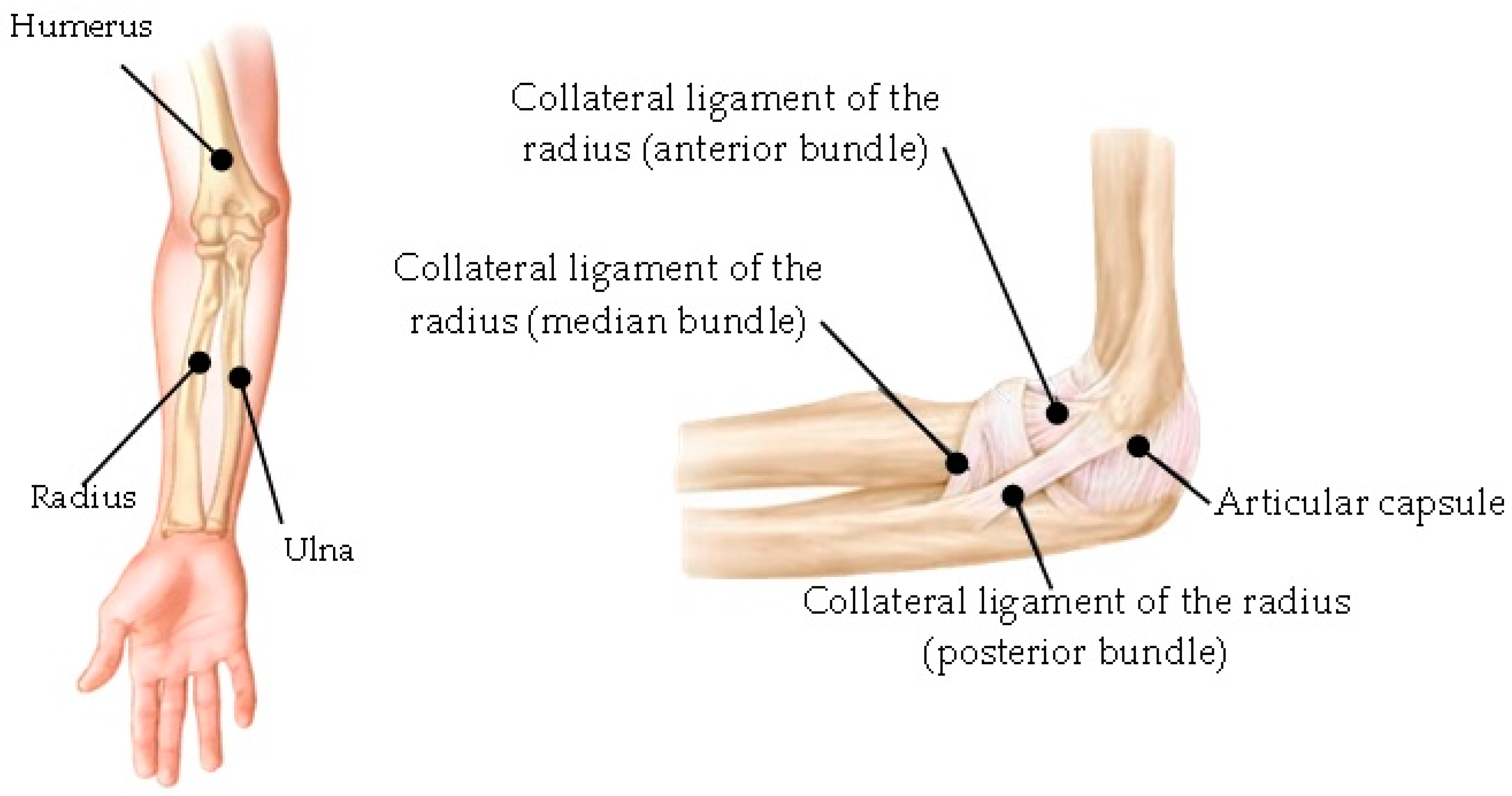
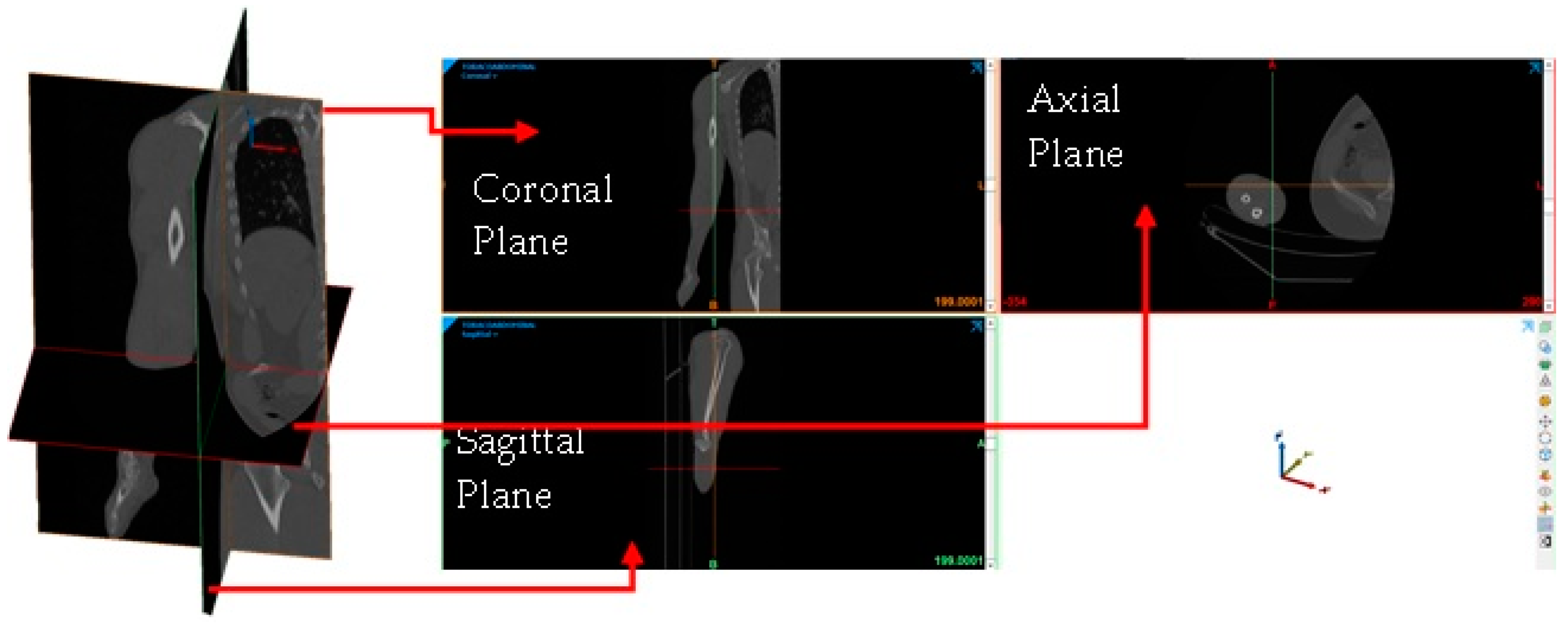
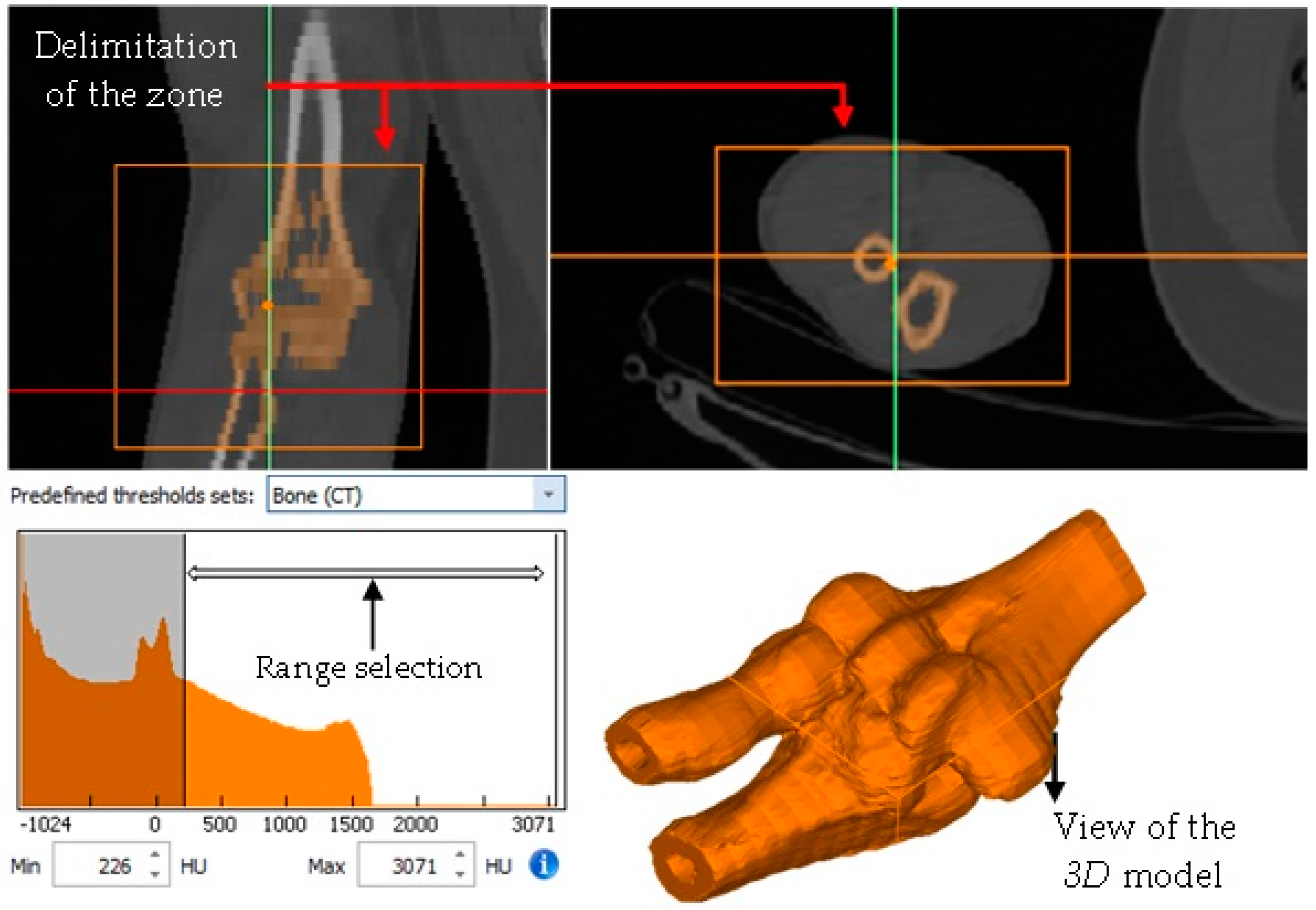
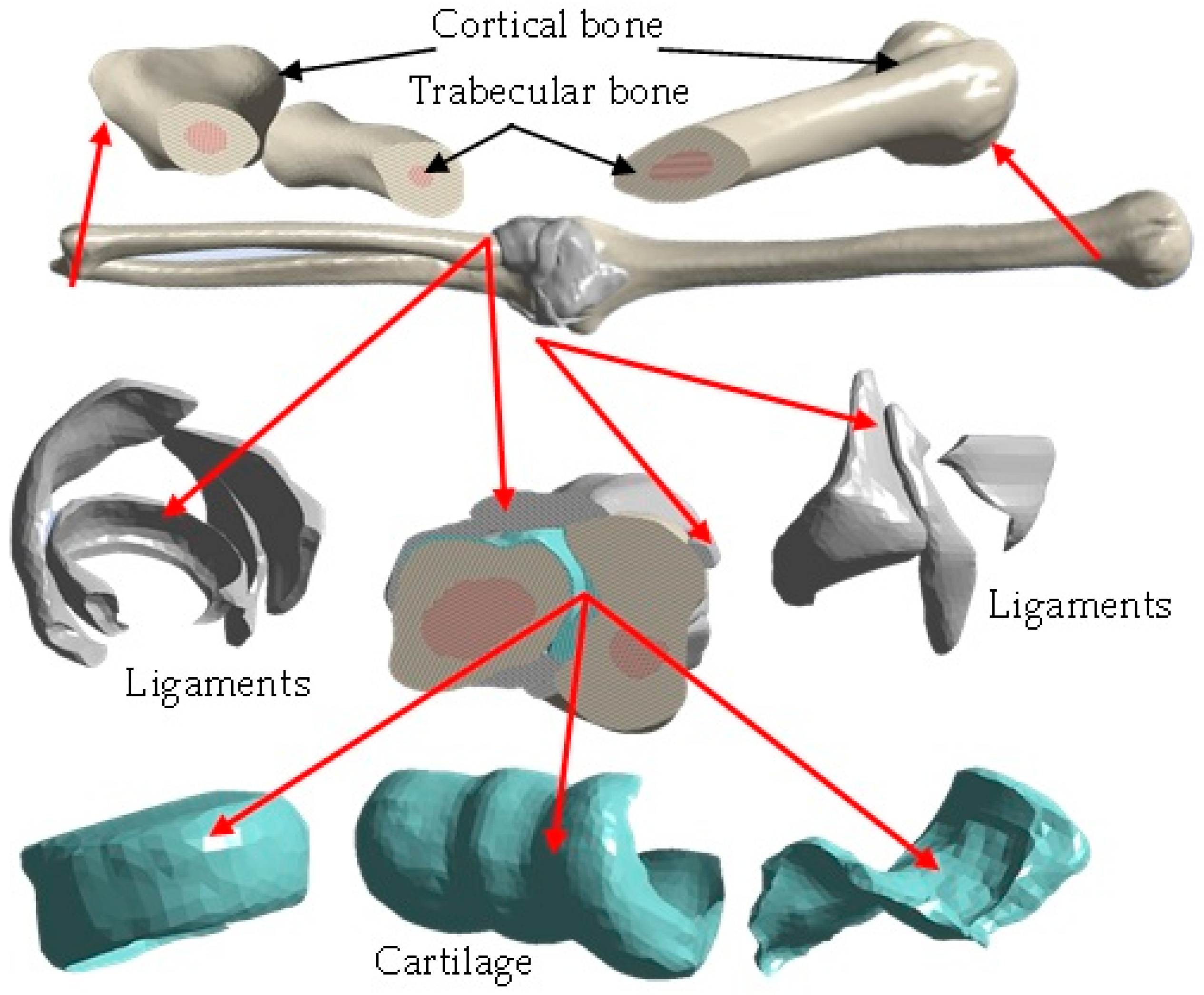
The methodology to develop a biomodel derives from a series of steps that involve computerized tomography in the DICOM format. For this study case, a computerized tomography scan of half of the patient’s torso was performed, where the working area to be characterized was enclosed (Figure 1) and included the elbow bones (humerus–radius–ulna), cartilage, and ligaments (Figure 2) [13]. Initially, the files obtained were imported into a computer program that can read the format. Next, a workspace was opened, consisting of four views (coronal, sagittal, axial, and total visualization of the model) where the slices that make up the tomography could be seen (Figure 3). It is possible to delimit the working area, and the software can automatically differentiate biological tissues. For this biomodel, a density mask range selection had a minimum value of 226 and a maximum value of 3071. The computational program can delimit the contour of the area of interest (Figure 4) without exceeding the established thickness (in this case, the cortical bone of the humerus, radius, and ulna). For trabecular bone, the density mask range was produced by an automatic procedure (cavity fill command), which identifies the cavity in the cortical bone and fills the space with soft material. However, the ligaments cannot be seen in computerized tomography, so ligaments were introduced in the biomodel by filling material in the space where the biological tissue is missing, which must be carried out manually (although the ligaments may present structural contact mismatch due to the complex shape or thickness of the structure) (Figure 5). Biomodel errors or mismatches are modified using reduction and smoothing commands for the component until the desired biological shape is correct. When generating contact between cortical bone and ligament, the most common thing that occurs is elements overlapping, which is resolved by performing a Boolean operation (removing the excess in material) and generating a uniformly smooth contact. Once the process has finished for each of the layers, the biomodel is operational and can be observed in the design window (Figure 6).
After the construction of the model, it was necessary to perform smoothing on the surface of each element. The procedure was completed by importing the model into another design software and producing a solid component (volume). The component elements were generated from discretization procedures of similar sizes and shapes. The model file was saved in an STL format, and the biomodel was exported to the Finite Element Method software and retained the same characteristics developed from the previous program because it was discretized as a solid mesh (which does not interfere with the defining time construction in the FEM discretization). The final biomodel was composed of different geometries—the cortical–trabecular bone, the cartilage (radius–ulna–humerus), and the elbow ligaments (capsule joint–collateral ligament and annular ligament of the radius–collateral ligament of the ulna)—which are assembled (representing the elbow joint) (Figure 6).
The development of the biomodeling of the elbow articulation (arm bones, ligaments, and cartilage) was performed as follows [14,15]:
  • Obtaining of the computerized axial tomography (upper limb).
  • Development of images in DICOM format.
  • Image importation into the Materialise Mimics® computer program.
  • Delimitation of the area of interest for the development of the biomodel (elbow).
  • Application of masks in the work area where the bones (cortical and trabecular) and cartilage will be represented.
  • Development of the capsule joint, implementing the mask around the contour between the bones that make up the elbow joint (humerus, radius, and ulna).
  • Development of ligaments through a mask that fills the gaps between the bones.
  • Application of smoothing to the surface of the biomodel.
  • Export of the biomodel to the 3-Matic Medical® program for the application of a mesh to obtain elements of similar size.
  • Solidification of the biomodel through re-meshing.
  • Exportation of the biomodel to a format with an extension compatible with the Ansys Workbench® program, which implements the Finite Element Method, for the development of numerical analysis.

3. Numerical Analysis

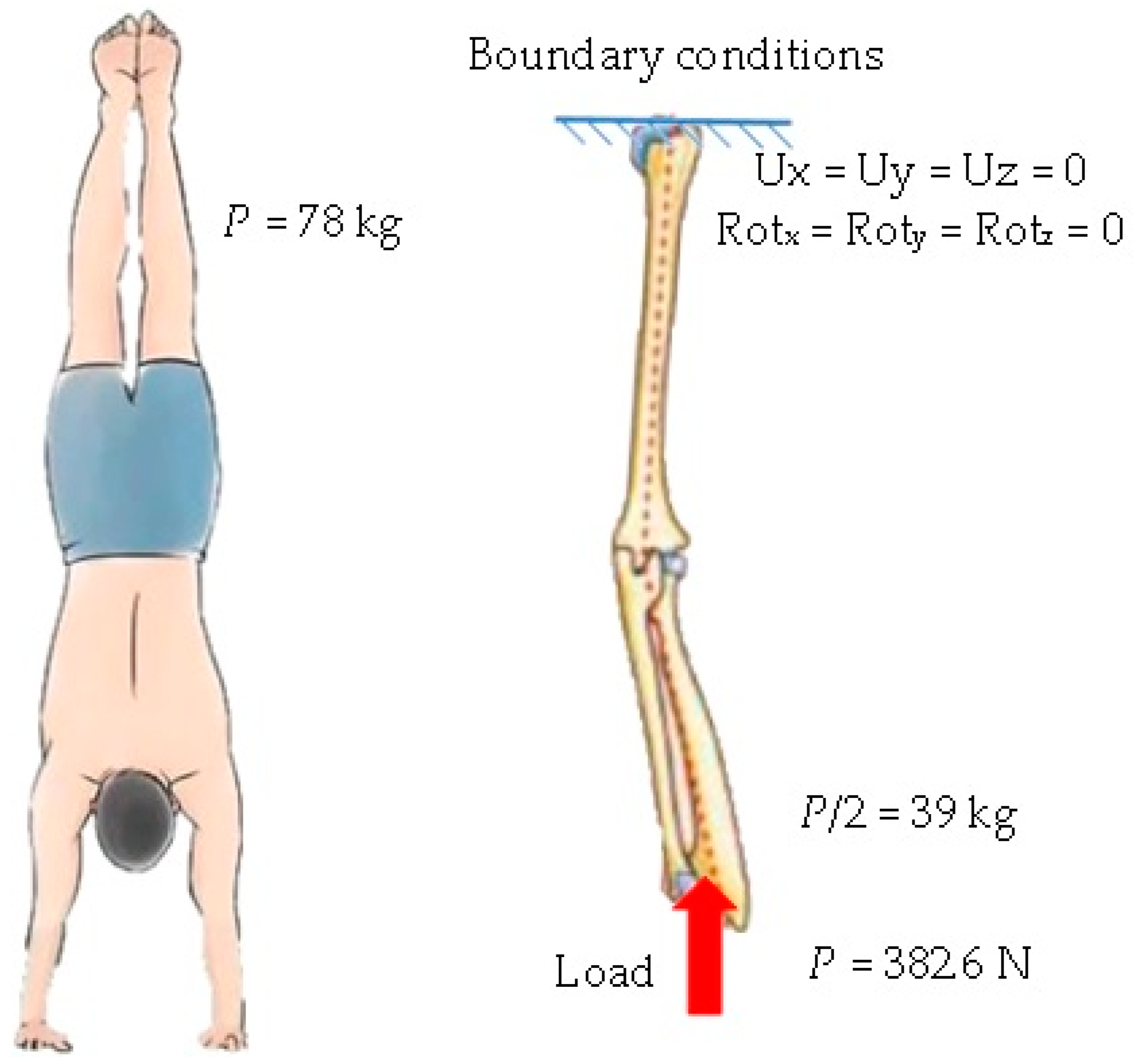
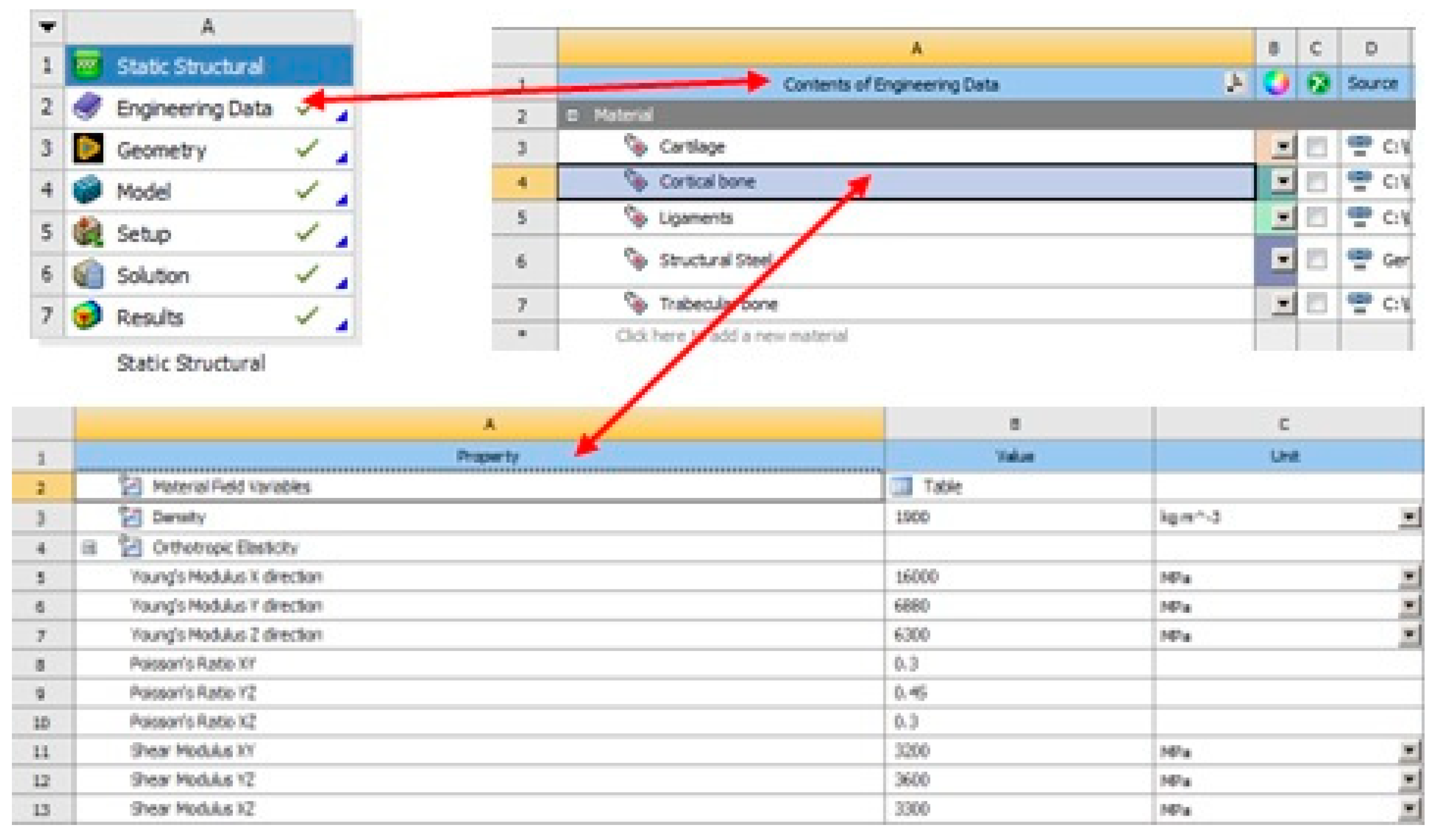
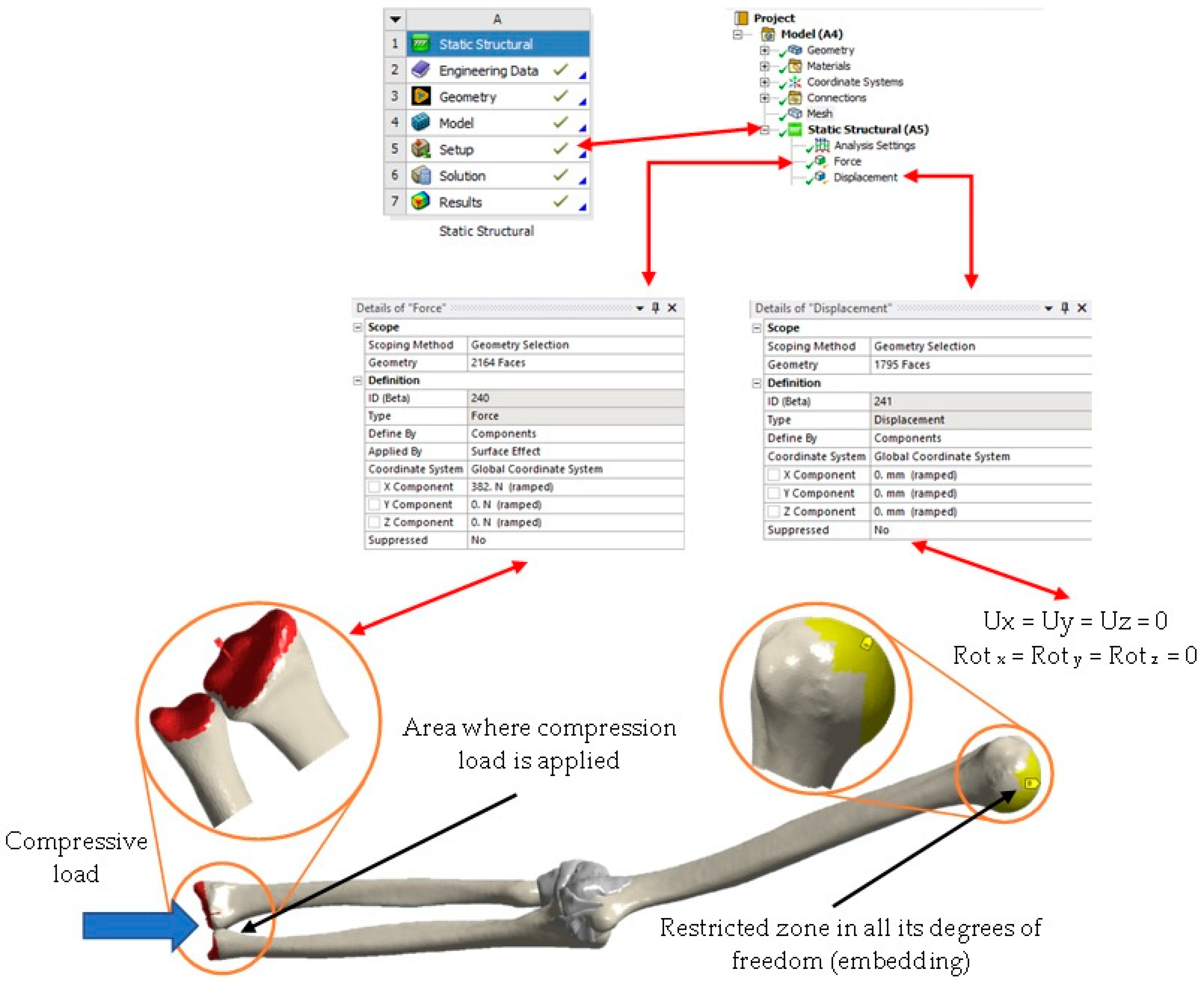
The execution of the numerical analysis was carried out in a computer program, Ansys Workbench® R1 2021, which applied a solution produced by the Finite Element Method using the previous numerical biomodel (representation of the biological tissue assembly). A structural static analysis was performed considering linear elastic behavior and orthotopic mechanical properties. Table 1, Table 2 and Table 3 show the mechanical properties characterizing the biological tissues (cortical bone, trabecular bone, ligaments, and cartilage) [16,17,18]. Figure 7 shows the loading and boundary condition configuration (free body diagram). Figure 8 shows the commands and the windows where the data in the tables are introduced. For discretization, high-order elements were selected, and the total assembly of the biomodel was composed of 17 solids, consisting of 857,746 nodes and 485,731 elements (Figure 9). The boundary conditions were given by the characteristics of an embedding, where the degrees of freedom were limited for the X, Y, and Z axes. Also, we restricted rotations in the XY, YZ, and XZ planes. In the humeral head part (Figure 10, yellow area), the load was applied on the distal part of the radius and ulna (on the longitudinal axis), which corresponds to the X axis (Figure 10, red area), as if the human being were standing on their hands. An individual weighing 78 kg was selected, and the weight was divided between the two arms on which the individual stood (conversion to Newtons was performed). The external agent was applied to the individual’s head (in the longitudinal axis), and the axial load applied was approximately 382.6 N.

4. Results

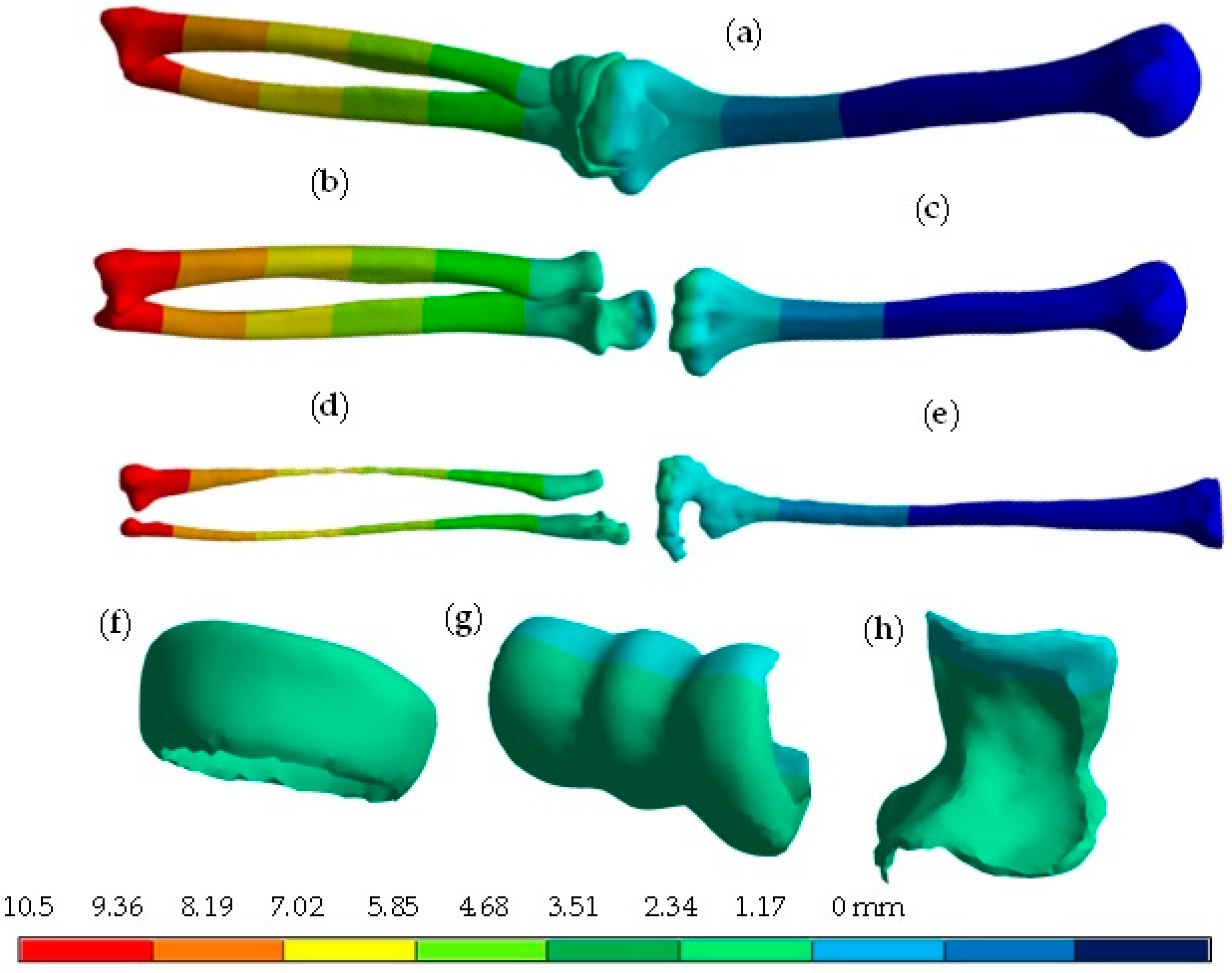
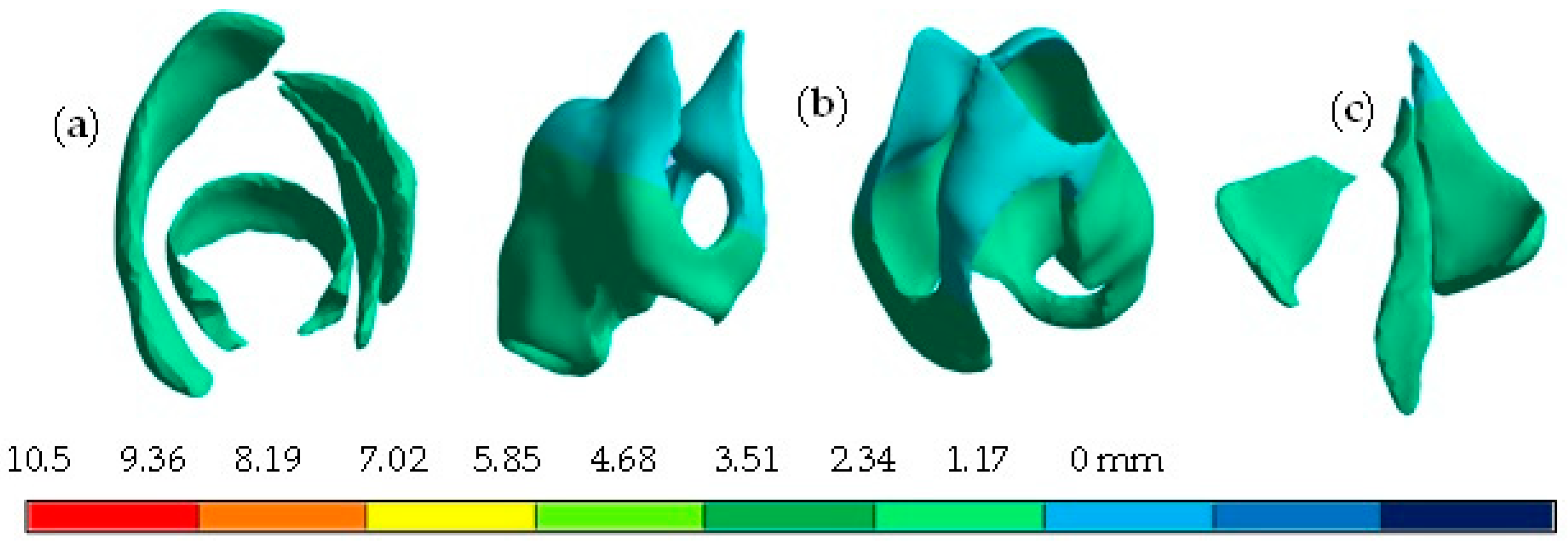
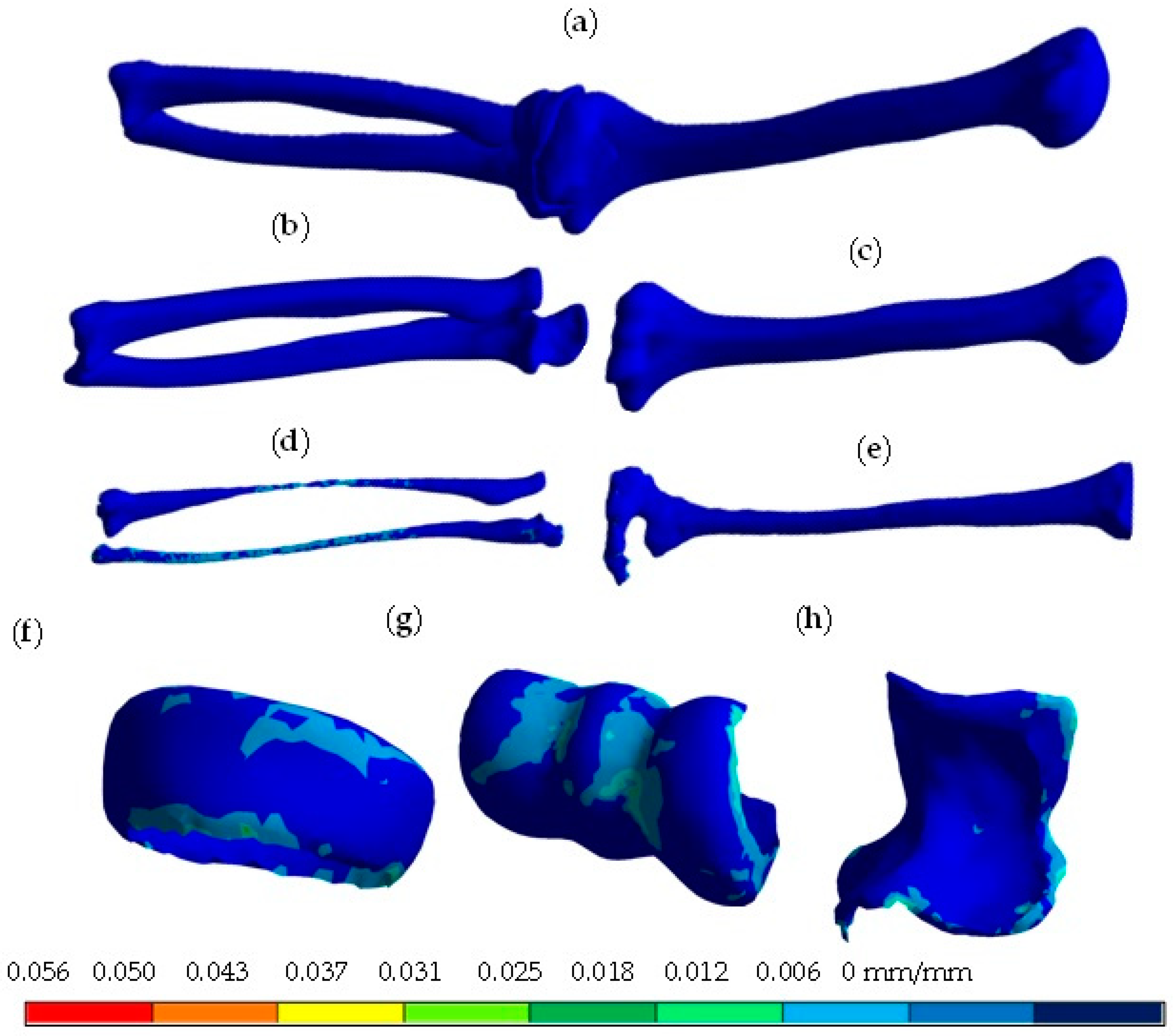
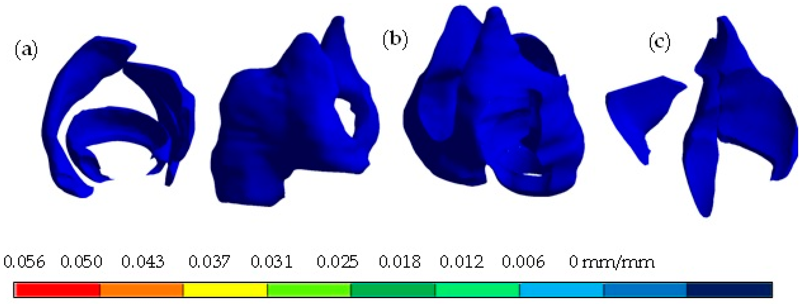
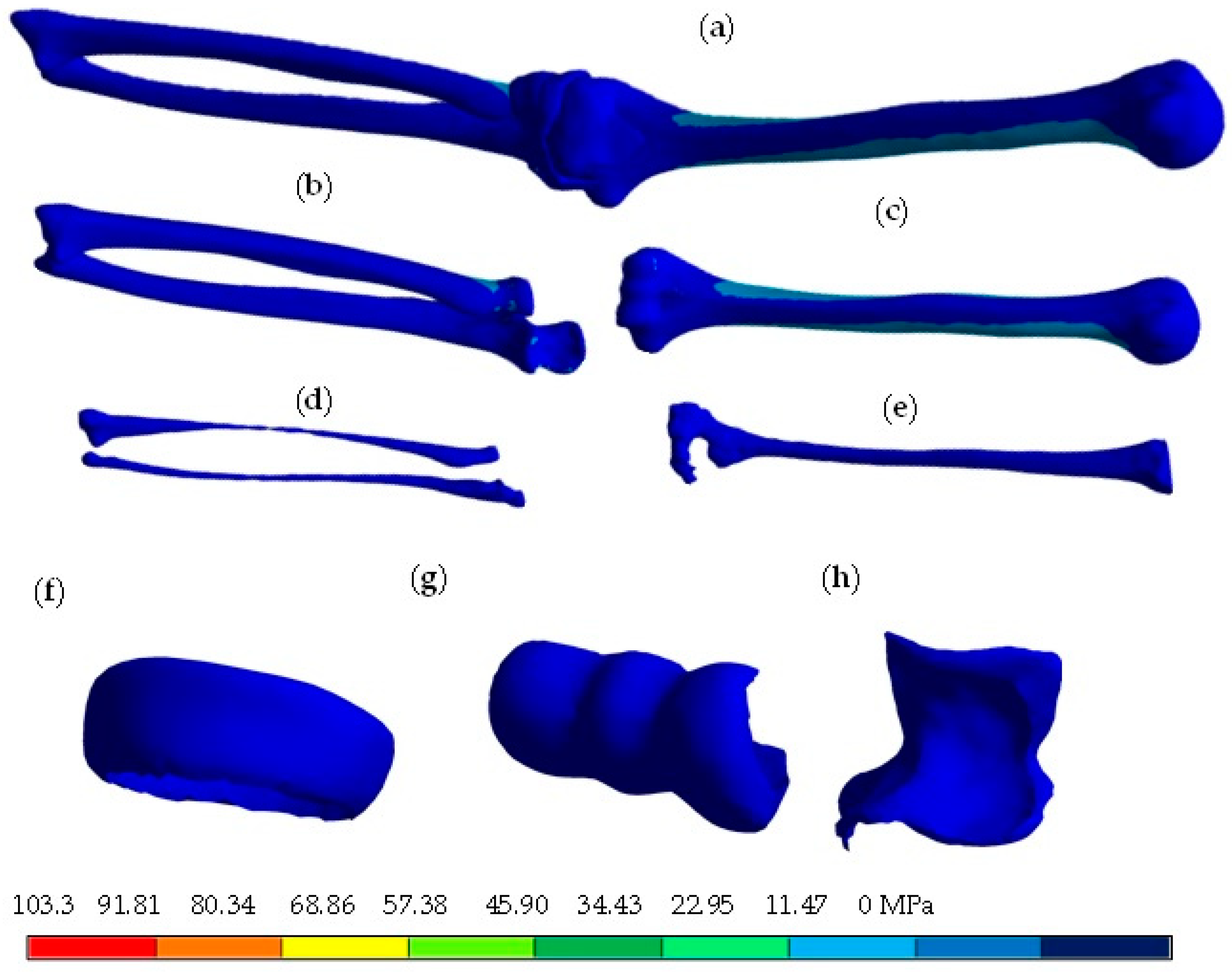
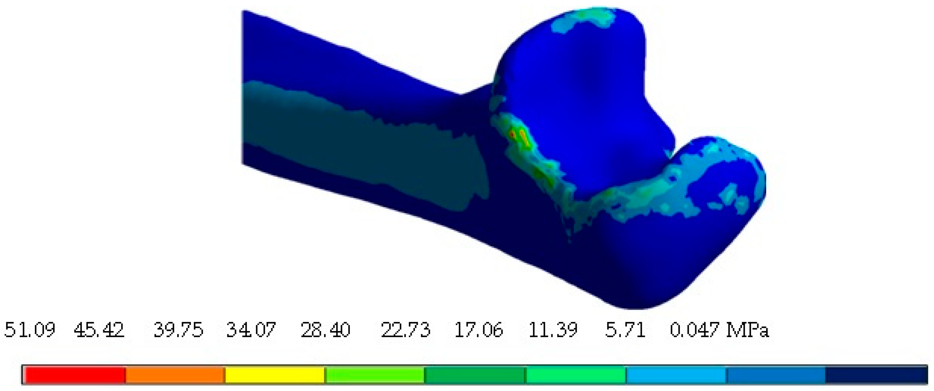
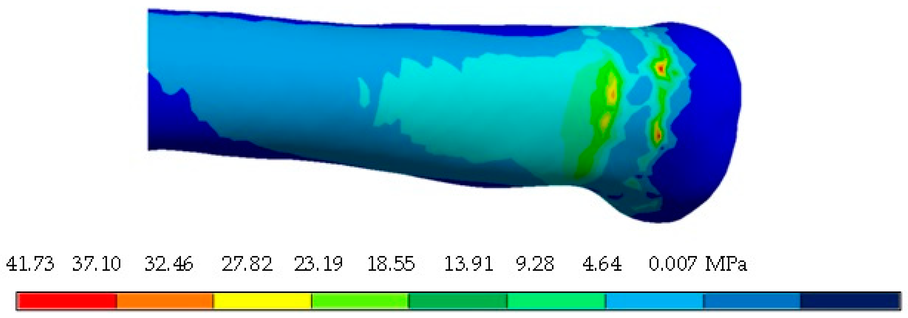
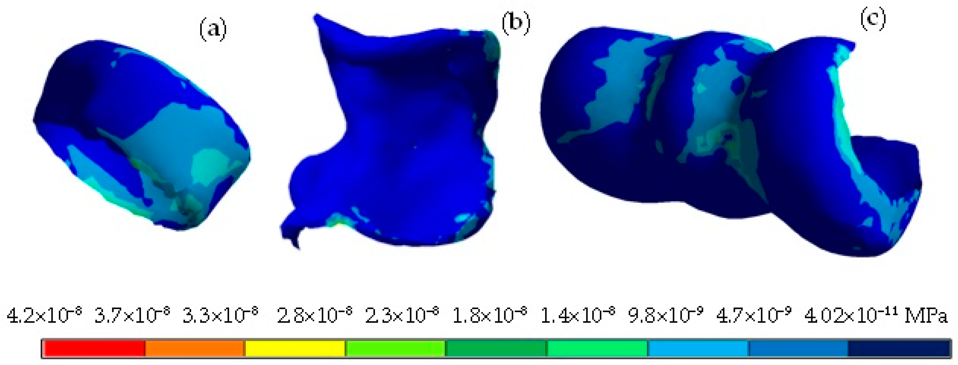
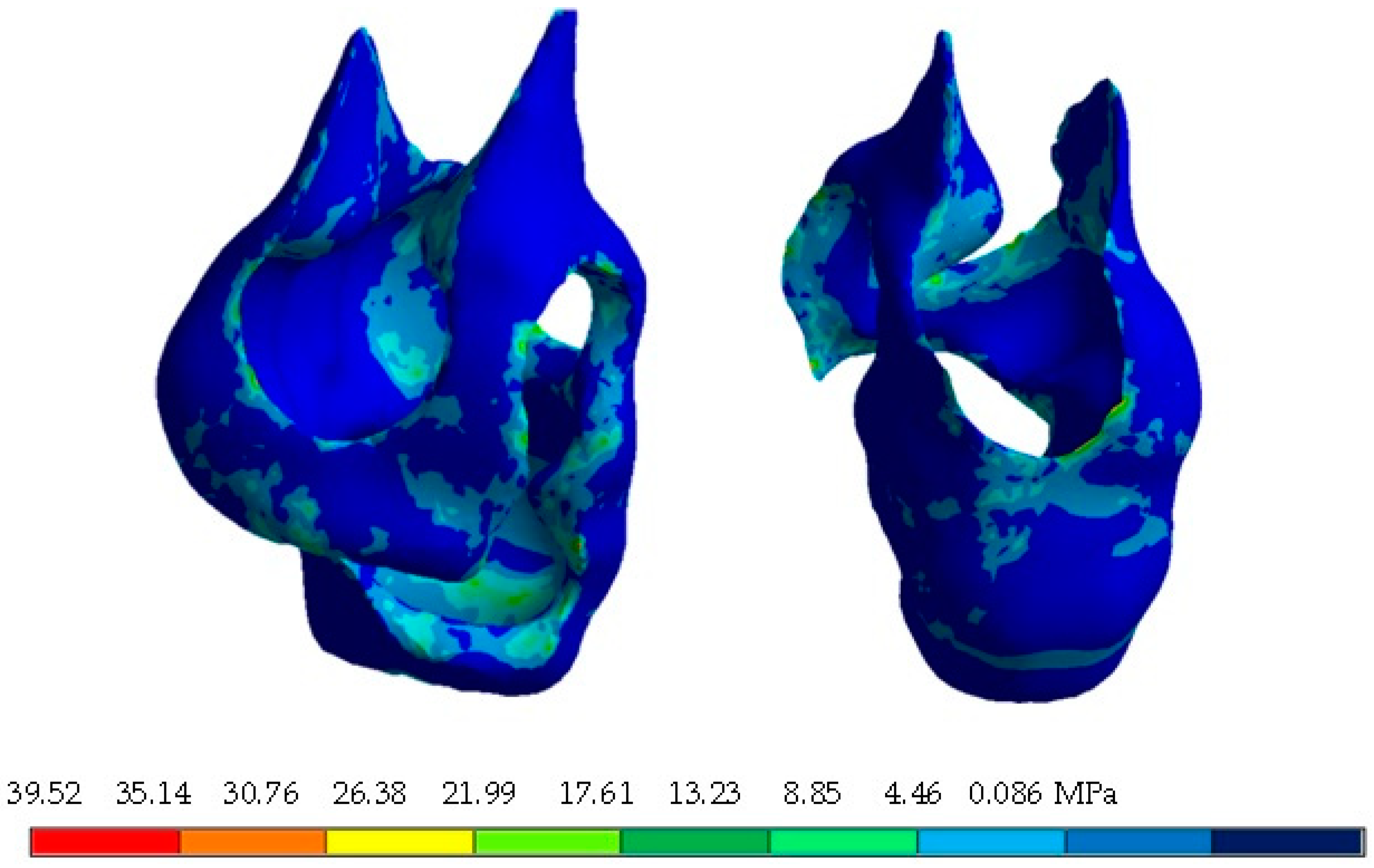
The numerical simulation results concerning the compressive load (along the longitudinal axis of the biomodel) show significant effects represented by the total displacement, general strains, and von Mises stress. Nevertheless, more results could be presented in the form of stresses, strains, and displacements to distinguish different effects, but for this study the above data show the highlighted consequences. Also, the results can be seen as a biomodel assembly conjunction or viewed individually for each element that makes up the biomodel (Figure 11, Figure 12, Figure 13, Figure 14, Figure 15, Figure 16, Figure 17, Figure 18, Figure 19, Figure 20 and Figure 21).

5. Discussion

Although there are currently different types of medical treatments for conditions that affect the human body, they have disadvantages because one cannot establish a diagnosis without compromising the integrity of the patient. Technology could be a supporting tool since the constant evolution in this area allows us to continue researching and providing solutions to different problems of the human body facing adversity. New technologies generate alternatives for surgical procedures, preventive methodologies, and corrective treatments. Numerical analyses are a reliable option for representing biological systems because they can simulate biological tissues in a three-dimensional manner, to which the conditions of its environment are applied. This study develops a methodology to produce a numerical biomodel for the simulation of the elbow joint and implementation of digital tools to perform a numerical evaluation (complemented with physics and structural mechanics knowledge). By developing a structural numerical evaluation of the healthy joint by the Finite Element Method, we obtained results showing how the structure behaves under the effect of compressive loading. The load distribution along the longitudinal axis and isochromatic changes can be distinguished where a maximum and minimum tensile stress is present, where the maximum represents the area prone to injury or even a fracture that could occur in this biological system. A biomodel is generated with characteristics that resemble the human body because it is developed from computerized axial tomography, which represents the bones, cartilage, and ligaments. Although the biofidelity of the biomodel can be questioned, it is clear that the characteristics of the biomodel represent 90% of the human morphology of the bone structure. It is worth mentioning that the internal structure that constitutes the biological tissue is too complex, so computerized tomography can be used to produce similar external dimensions. To quantify the error between the human component and the biomodel, it would be necessary to extract the human bone and obtain the mismatch percentage. The research objective was to produce biomodels and numerical evaluations so that diagnosis can be developed without affecting the integrity of the patient. Regarding the benefits of carrying out this type of research project where a biomodel is used, there is no doubt that it can cover several areas where medical diagnoses are implemented for the development of preventive and corrective treatments for a specific condition that affects the bone and joint structures of the human body. According to the results, the maximum total displacement occurs when the compressive load is applied, causing the bones (radius and ulna) to tend to separate at the interosseous membrane. Also, the strain describes the load tendency effect that affects the cartilage in the trochlea of the humerus zone. These results indicate the areas where the generation of cartilage wear begins. Finally, regarding the general stress distribution data, there is a change in isochromatic colors that is shown at the longitudinal part of the humerus and the section of the proximal part of the radius, initiating the volume reduction of these elements, and these changes tend to generate small lesions or even a crack in the bone. To better highlight the isochromatic changes that demonstrate how the stress is distributed in each component, an individual evaluation was performed. With this evaluation, the critical zones showing the maximum stresses are better appreciated, with smaller stress fields in the ulna, radius, and humerus. It can be stated that the affected area is located at the capsule joint. It can be concluded that at these points the load exceeds the structural resistance of the component. Also, there will be a separation between the capsule joint and the cortical bone, which can generate a joint effusion that causes pain. The authors have carried out projects where different methodologies were used for the development of biomodels applied to rehabilitation work and bone diseases, where it is considered an innovative process in medicine, biology, and dentistry [19,20,21,22,23,24].

6. Conclusions

The numerical evaluation presented has the advantage that the biomodel developed has a biofidelity that allows it to represent the morphological characteristics of the bones that constitute the elbow joint. The biological system is considered a continuous solid that has a defined volume suitable for developing the numerical analysis that applies the Finite Element Method. The results obtained showed the presence of stress concentrators and areas prone to injury or fractures. The von Misses stress results showed that, for the general analysis of the assembly, a slight isochromatic change is present in the proximal part of the humerus. The numerical analysis of individual components shows how the maximum stress is concentrated in the area where the ligaments are related to the bones. On the other hand, it was observed in the analysis that the elastic limit of the biological system was not exceeded. The results obtained and the behavior shown in this case (by the biomodel) can be validated by performing experimental tests. However, this is nearly impossible due to the cost, the risk to the patient, and established hygienic regulations. Numerical analysis can avoid experimental procedures, reduce costs, reduce time, and could be closer to reality. This shows that the application of these technological tools can influence different medical areas. All the results obtained are shown in Appendix A, Table A1, Table A2, Table A3 and Table A4. With this type of model, one can also add and simulate fractures in the bone or injuries that affect the joint, such as injuries to the ligaments or cartilage, because the human body degenerates as it completes its life cycle. Also, characterizing wear on the elbow joint is generated by developing repetitive or overextension movements that are commonly generated by the practice of sport, directly affecting the cartilage. Additionally, in the field of sports, the representation of bones with this method can be used to measure how the biological tissue is degenerating by carrying out a previous study when the joint is healthy or presents a previous injury and implementing a measurement period, so that at the end of this a new model is made to observe how much the biological tissue that is being studied has degenerated. It can also be used when a fracture occurs to determine how it is regenerated during the healing process, with the objective of determining whether there are malformations during this period. Finally, this biomodel can be used to generate a prosthesis design in a personalized manner. It can even develop bone prototypes using 3D printers with the purpose of developing bone models implementing biocompatible materials.

Author Contributions

Conceptualization, D.M.-A., G.U.-S. and B.R.-Á.; methodology, D.M.-A., G.U.-S., B.R.-Á. and G.M.U.-C.; validation, D.M.-A., G.U.-S., B.R.-Á., M.M.-M. and A.T.-E.; formal analysis, D.M.-A., G.U.-S., B.R.-Á. and M.I.C.-C.; investigation, D.M.-A., G.U.-S., B.R.-Á. and G.M.U.-C.; resources, D.M.-A., G.U.-S., B.R.-Á. and J.M.G.-C.; writing—original draft preparation, D.M.-A., G.U.-S., B.R.-Á. and A.S.-C.; writing—review and editing, D.M.-A., G.U.-S., B.R.-Á. and A.U.-L.; visualization, D.M.-A., G.U.-S., B.R.-Á. and M.I.C.-C.; supervision, D.M.-A., G.U.-S. and B.R.-Á.; project administration, D.M.-A., G.U.-S., B.R.-Á. and G.M.U.-C. All authors have read and agreed to the published version of the manuscript.

Funding

This research received no external funding.

Institutional Review Board Statement

Not applicable.

Informed Consent Statement

Not applicable.

Data Availability Statement

Not applicable.

Acknowledgments

The authors gratefully acknowledge the Instituto Politécnico Nacional, Consejo Nacional de Humanidades Ciencias y Tecnologías for supporting this research and Francisco Carrasco Hernández.

Conflicts of Interest

The authors declare no conflict of interest.

Appendix A

Table A1. Summary of general results of numerical evaluation of the humerus.
ConceptCortical BoneTrabecular BoneCartilage
MaximumMinimumMaximumMinimumMaximumMinimum
Total displacement (mm)3.8003.7003.873.32
Directional displacement, X axis (mm)1.16−0.211.02−0.0711.030.02
Directional displacement, Y axis (mm)0.010−1.570.008−1.51−1.42−1.58
Directional displacement, Z axis (mm)0.002−3.460.007−3.28−2.97−3.53
Elastic Strain0.005−1.85 × 10−80.0155.69 × 10−50.0560.0001
Elastic Strain, X axis0.001−0.0020.007−0.0050.018−0.023
Elastic Strain, Y axis0.0008−0.00060.008−0.0060.014−0.005
Elastic Strain, Z axis0.001−0.0020.005−0.0050.025−0.019
Von Mises stress (MPa)33.5011.6504.02 × 10−83.68 × 10⁻¹¹
Nominal X-axis stress (MPa)25.46−36.6211.28−8.861.35 × 10−81.69 × 10⁻⁸
Nominal Y-axis stress (MPa)10.99−6.802.47−2.351.14 × 10−8−4.67 × 10⁻⁹
Nominal Z-axis stress (MPa)15.68−15.854.22−4.241.95 × 10−81.44 × 10⁻⁸
Maximum principal stress (MPa)27.29−5.5012.98−1.272.50 × 10−8−8.46 × 10⁻¹⁰
Middle principal stress (MPa)10.78−10.632.67−2.256.04 × 10−9−2.47 × 10⁻⁹
Minimum principal stress (MPa)5.63−37.191.15−10.799.68 × 10−10−2.13 × 10⁻⁸
XY shear stress (MPa)7.89−6.842.39−2.097.73 × 10−9−8.98 × 10⁻⁹
YZ shear stress (MPa)6.57−8.471.92−2.455.06 × 10−9−7.18 × 10⁻⁹
XZ shear stress (MPa)13.45−11.044.20−5.529.51 × 10−9−1.34 × 10⁻⁸
Table A2. Summary of general results of numerical evaluation of the ulna.
ConceptCortical BoneTrabecular BoneCartilage
MaximumMinimumMaximumMinimumMaximumMinimum
Total displacement (mm)10.263.2610.073.684.113.31
Directional displacement, X axis (mm)1.990.081.820.370.920.07
Directional displacement, Y axis (mm)−1.41−2.90−1.52−2.85−1.43−1.61
Directional displacement, Z axis (mm)−2.90−9.69−3.32−9.50−2.97−3.68
Elastic Strain0.0065.92 × 10−60.0170.00010.042.87 × 10−5
Elastic Strain, X axis0.002−0.0020.009−0.0070.02−0.015
Elastic Strain, Y axis0.0007−0.00060.001−0.0020.004−0.003
Elastic Strain, Z axis0.0010.0020.006−0.0040.017−0.017
Von Mises stress (MPa)48.72014.4103.43 × 10−81.75 × 10⁻¹¹
Nominal X-axis stress (MPa)35.08−47.6412.72−9.831.73 × 10−8−1.15 × 10⁻⁸
Nominal Y-axis stress (MPa)7.83−10.742.25−2.423.84 × 10−9−2.84 × 10⁻⁹
Nominal Z-axis stress (MPa)11.63−15.833.97−3.551.37 × 10−8−1.35 × 10⁻⁸
Maximum principal stress (MPa)37.32−5.1913.79−1.342.23 × 10−8−2.11 × 10⁻¹⁰
Middle principal stress (MPa)8.75−11.183.55−3.456.17 × 10−9−3.82 × 10⁻⁹
Minimum principal stress (MPa)4.85−50.811.22−10.076.83 × 10−10−1.81 × 10⁻⁸
XY shear stress (MPa)7.95−7.143.18−5.156.12 × 10−9−6.36 × 10⁻⁹
YZ shear stress (MPa)9.47−8.482.08−2.787.35 × 10−9−4.25 × 10⁻⁹
XZ shear stress (MPa)12.52−14.167.12−5.061.31 × 10−89.61 × 10⁻⁹
Table A3. Summary of overall results of numerical evaluation of radius.
ConceptCortical BoneTrabecular BoneCartilage
MaximumMinimumMaximumMinimumMaximumMinimum
Total displacement (mm)10.543.8510.344.004.163.82
Directional displacement, X axis (mm)2.300.662.180.801.180.64
Directional displacement, Y axis (mm)−1.54−3.01−1.57−2.96−1.53−1.61
Directional displacement, Z axis (mm)−3.44−9.88−3.56−9.69−3.40−3.67
Elastic Strain0.0055.34 × 10−60.0165.34 × 10−60.030.0001
Elastic Strain, X axis0.002−0.0022.07−3.480.008−0.010
Elastic Strain, Y axis0.0005−0.00075.83−5.570.006−0.0010
Elastic Strain, Z axis0.002−0.0010.009−0.0070.011−0.009
Von Mises stress (MPa)37.32014.2202.16 × 10−87.42 × 10⁻¹¹
Nominal X-axis stress (MPa)38.1136.659.70−8.776.73 × 10−6−8.00 × 10⁻⁹
Nominal Y-axis stress (MPa)7.01−7.962.07−3.485.22 × 10−9−1.65 × 10⁻⁹
Nominal Z-axis stress (MPa)15.17−13.845.83−5.579.33 × 10−9−7.03 × 10⁻⁹
Maximum principal stress (MPa)41.53−4.9911.56−1.211.56 × 10−8−4.33 × 10⁻¹⁰
Middle principal stress (MPa)8.40−7.452.02−2.374.52 × 10−94.23 × 10⁻⁹
Minimum principal stress (MPa)5.16−37.000.93−11.29.94 × 10−10−1.13 × 10⁻⁸
XY shear stress (MPa)10.83−5.843.87−2.332.72 × 10−9−4.05 × 10⁻⁹
YZ shear stress (MPa)4.17−11.382.77−2.408.94 × 10−9−2.24 × 10⁻⁹
XZ shear stress (MPa)−11.09−11.097.52−4.363.15 × 10−9−1.77 × 10⁻⁸
Table A4. Summary of general results of numerical assessment of the elbow joint.
ConceptCapsule JointLigaments of the RadiusLigaments of the Ulna
MaximumMinimumMaximumMinimumMaximumMinimum
Total displacement (mm)4.532.764.203.514.193.36
Directional displacement, X axis (mm)1.25−0.011.270.380.43−0.08
Directional displacement, Y axis (mm)−1.26−1.66−1.44−1.61−1.45−1.65
Directional displacement, Z axis (mm)−2.41−3.87−3.06−3.713.03−3.83
Elastic Strain0.0062.00 × 10−50.0172.09 × 10−60.0121.08 × 10−6
Elastic Strain, X axis0.004−0.004−0.008−0.0060.006−0.004
Elastic Strain, Y axis0.002−0.0010.008−0.0040.001−0.001
Elastic Strain, Z axis0.003−0.0040.005−0.0070.004−0.005
Von Mises stress (MPa)37.660103.3073.490
Nominal X-axis stress (MPa)34.22−40.48102.6−39.2830.39−38.10
Nominal Y-axis stress (MPa)17.71−22.1052.39−21.2015.36−20.77
Nominal Z-axis stress (MPa)18.15−25.8165.00−62.1934.97−20.42
Maximum principal stress (MPa)34.32−12.02115.19−15.5238.52−7.87
Middle principal stress (MPa)18.96−21.6663.34−28.3724.06−18.40
Minimum principal stress (MPa)11.27−43.9539.42−94.4012.73−49.20
XY shear stress (MPa)15.52−12.9125.26−26.157.73−17.11
YZ shear stress (MPa)7.54−9.1442.17−5.9512.38−28.54
XZ shear stress (MPa)13.41−19.7528.34−25.3319.07−14.26

References

  1. Willing, R.T.; Lalone, E.A.; Shannon, H.; Johnson, J.A.; King, G.J.W. Validation of a finite element model of the human elbow for determining cartilage contact mechanics. J. Biomech. 2013, 46, 1767–1771. [Google Scholar] [CrossRef] [PubMed]
  2. Garzón-Alvarado, D.A.; Duque-Daza, C.A.; Ramírez-Martínez, A.M. On the emergence of biomechanics and computational mechanobiology: Computational experiments and recent findings. Rev. Cuba. Investig. Bioméd. 2009, 28, 83–101. [Google Scholar]
  3. Urbanowieza, E.M.; Ramíreza, E.I.; Ruiz, O.; Ortiza, A. Analysis by finite element parcel of a Thompson® hip prosthesis under four different load conditions. In Proceedings of the XXI Annual International Congress of the SOMIM, Pachuca, México, 22–24 September 2021; pp. 24–31. [Google Scholar]
  4. López-Liévano, A.; López-Liévano, D.R.; Caicedo-Ortiz, H.E.; González-Rebattú, A. Biomodeling of the components of the human middle ear using magnetic resonance imaging. Scientist 2017, 21, 3–8. [Google Scholar]
  5. Kumar, S.; Kumar, J. A review on application of finite element modelling in bone biomechanics. Perspect. Sci. 2016, 8, 696–698. [Google Scholar]
  6. Goel, V.K.; Singh, D.; Bijlani, V. Contact areas in human elbow joints. J. Biomech. Eng. 1982, 104, 169–175. [Google Scholar] [CrossRef]
  7. Lohfeld, S.; Barron, V.; McHugh, P.E. Biomodels of Bone: A Review. Ann. Biomed. Eng. 2005, 33, 1295–1311. [Google Scholar] [CrossRef]
  8. Ruiz-Santiago, F.; Castellano-García, M.; Guzmán-Álvarez, L.; Tello-Moreno, M. Computed tomography and magnetic resonance imaging in painful diseases of the spine; Respective contributions and controversies. Radiology 2011, 53, 116–133. [Google Scholar]
  9. Cristea, A.F. Mechanical stress and strain properties, regarding the elbow joint. Acta Tech. Napoc.-Ser. Appl. Math. Mech. Eng. 2014, 57, 179–188. [Google Scholar]
  10. Jardini, A.L.; Larosa, M.A.; Filho, R.M.; Zavaglia, C.A.D.C.; Bernardes, L.F.; Lambert, C.S.; Kharmandayan, P. Cranial reconstruction: 3D biomodel and custom-built implant created using additive manufacturing. J. Cranio-Maxillofac. Surg. 2014, 42, 1877–1884. [Google Scholar] [CrossRef]
  11. Oliveira, M.; Sooraj Hussain, N.; Dias, A.G.; Lopes, M.A.; Azevedo, L.; Zenha, H.; Santos, J.D. 3-D biomodelling technology for maxillofacial reconstruction. Mater. Sci. Eng. C 2008, 28, 1347–1351. [Google Scholar] [CrossRef]
  12. Nareliya, R.; Kumar, V. Finite element application to a femur bone: A review. J. Biomed. Bioeng. 2012, 3, 57–62. [Google Scholar]
  13. Cisneros-Hidalgo, Y.; González-Carbonell, R.; Ortiz-Prado, A.; Jacobo-Almendáriz, V.; Puente-Álvarez, A. Modelo mechanobiological of a human tibia to determine its response to external mechanical stimuli. Cuba. J. Biomed. Res. 2015, 34, 54–63. [Google Scholar]
  14. Mastache-Miranda, O.A.; Urriolagoitia-Sosa, G.; Marquet-Rivera, R.A. Three-dimensional reconstruction for use in medicine and biomechanics. MOJ Appl. Bionics Biomech. 2018, 2, 310–331. [Google Scholar]
  15. Marquet-Rivera, R.A.; Urriolagoitia-Sosa, G.; Romero-Ángeles, B.; Vázquez-Feijoo, J.A.; Urriolagoitia-Calderón, G. Computational biomodelling and numerical analysis as means of diagnostic and odontological prognosis. MOJ Appl. Bionics Biomech. 2018, 2, 262–263. [Google Scholar]
  16. Wu, D.; Isaksson, P.; Fergusson, S.J.; Persson, C. Young´s modulus of trabecular bone at the tissue level: A review. Acta Biomater. 2018, 78, 1–12. [Google Scholar] [CrossRef] [PubMed]
  17. Flores-Renteria, M.A.; Ortíz-Domínguez, M.; Cruz-Avilés, A.; López-Sánchez, F. Bone mechanics: A review of bone remodeling, Ingenuity and Consciousness. Sci. Bull. Super. Sch. Ciudad. Sahagún 2018, 9, 1–15. [Google Scholar]
  18. Mendoza, A. Study of the mechanical properties of the bone system. J. Eng. Res. 1991, 23, 14–19. [Google Scholar]
  19. Martinez-Mondragon, M.; Urriolagoitia-Sosa, G.; Romero-Ángeles, B.; Maya-Anaya, D.; Martínez-Reyes, J.; Gallegos-Funes, F.J.; Urriolagoitia-Calderón, G.M. Numerical Analysis of Zirconium and Titanium Implants under the Effect of Critical Masticatory Load. Materials 2022, 15, 7843. [Google Scholar] [CrossRef]
  20. Hernández-Vázquez, R.A.; Romero-Ángeles, B.; Urriolagoitia-Sosa, G.; Vázquez-Feijoo, J.A.; Vázquez-López, Á.J.; Urriolagoitia-Calderón, G. Numerical analysis of masticatory forces on a lower first molar considering the contact between dental tissues. Appl. Bionics Biomech. 2018, 2018, 4196343. [Google Scholar] [CrossRef] [Green Version]
  21. Marquet-Rivera, R.A.; Urriolagoitia-Sosa, G.; Hernández-Vázquez, R.A.; Romero-Ángeles, B.; Mastache-Miranda, O.A.; Urriolagoitia-Calderón, G. High biofidelity 3D biomodel reconstruction from soft and hard tissues (knee), FEM, and 3D printing: A three-dimensional methodological proposal. BioMed Res. Int. 2021, 2021, 6688164. [Google Scholar]
  22. Hernández-Vázquez, R.A.; Urriolagoitia-Sosa, G.; Marquet-Rivera, R.A.; Romero-Angeles, B.; Mastache-Miranda, O.A.; Vázquez-Feijoo, J.A.; Urriolagoitia-Calderon, G. High-biofidelity biomodel generated from three-dimensional imaging (cone-beam computed tomography): A methodological proposal. Comput. Math. Methods Med. 2020, 2020, 4292501. [Google Scholar] [CrossRef] [PubMed] [Green Version]
  23. Marquet-Rivera, R.A.; Urriolagoitia-Sosa, G.; Romero-Ángeles, B.; Hernández-Vázquez, R.A.; Mastache-Miranda, O.A.; Cruz-López, S.; Urriolagoitia-Calderón, G. Numerical Analysis of the ACL, with Sprains of Different Degrees after Trauma. Comput. Math. Methods Med. 2021, 2021, 2109348. [Google Scholar] [CrossRef] [PubMed]
  24. Hernández-Vázquez, R.A.; Romero-Ángeles, B.; Urriolagoitia-Sosa, G.; Vázquez-Feijoo, J.A.; Marquet-Rivera, R.A.; Urriolagoitia-Calderón, G. Mechanobiological analysis of molar teeth with carious lesions through the finite element method. Appl. Bionics Biomech. 2018, 2018, 1815830. [Google Scholar] [CrossRef] [PubMed] [Green Version]
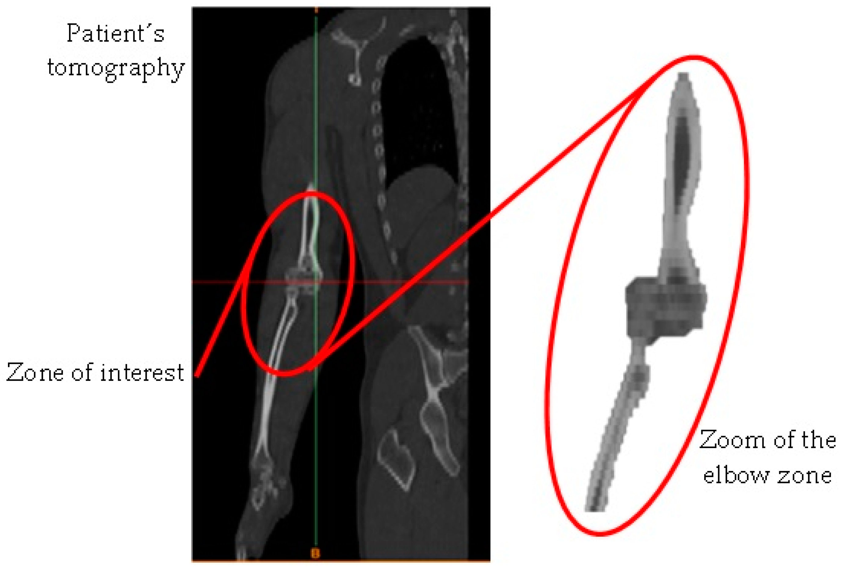
Figure 1. Patient’s tomography.
Applsci 13 08903 g001
Figure 2. Arm components.
Applsci 13 08903 g002
Figure 3. View of the work areas for the biomodel design.
Applsci 13 08903 g003
Figure 4. Delimitation of the working area.
Applsci 13 08903 g004
Figure 5. Initial biomodel.
Applsci 13 08903 g005
Figure 6. Solid model geometry.
Applsci 13 08903 g006
Figure 7. Loading free body diagram.
Applsci 13 08903 g007
Figure 8. Data windows in Ansys Workbench®.
Applsci 13 08903 g008
Figure 9. Commands to generate the discretization in the model.
Applsci 13 08903 g009
Figure 10. Application of boundary and load conditions to the model.
Applsci 13 08903 g010
Figure 11. Total displacement results. (a) Complete model of the elbow joint. (b) Radius–ulna (cortical bone). (c) Humerus cortical bone. (d) Radius–ulna (trabecular bone). (e) Humerus trabecular bone. (f) Radius cartilage. (g) Cartilage of the humerus. (h) Ulna cartilage.
Applsci 13 08903 g011
Figure 12. Total displacement results. (a) Collateral and annular ligaments of the radius. (b) Elbow joint capsule (front–rear view). (c) Collateral ligaments of the ulna.
Applsci 13 08903 g012
Figure 13. Total elastic strain results. (a) Complete model of the elbow joint. (b) Radius–ulna (cortical bone). (c) Humerus cortical bone. (d) Radius–ulna (trabecular bone). (e) Humerus trabecular bone. (f) Radius cartilage. (g) Cartilage of the humerus. (h) Ulna cartilage.
Applsci 13 08903 g013
Figure 14. Total elastic strain results. (a) Collateral and annular ligaments of the radius. (b) Elbow joint capsule (front–rear view). (c) Collateral ligaments of the ulna.
Applsci 13 08903 g014
Figure 15. Von Mises’s stress results. (a) Complete model of the elbow joint. (b) Radius–ulna (cortical bone). (c) Humerus cortical bone. (d) Radius–ulna (trabecular bone). (e) Humerus trabecular bone. (f) Radius cartilage. (g) Cartilage of the humerus. (h) Ulna cartilage.
Applsci 13 08903 g015
Figure 16. Von Mises’s stress results. (a) Collateral and annular ligaments of the radius. (b) Elbow joint capsule (front–rear view). (c) Collateral ligaments of the ulna.
Applsci 13 08903 g016
Figure 17. Von Mises’s stress results for individual analysis of the ulna.
Applsci 13 08903 g017
Figure 18. Von Mises’s stress results for individual analysis of the radius.
Applsci 13 08903 g018
Figure 19. Von Mises’s stress results for individual analysis of the humerus.
Applsci 13 08903 g019
Figure 20. Von Mises’s stress results for individual cartilage analysis: (a) radius, (b) ulna, (c) humerus.
Applsci 13 08903 g020
Figure 21. Von Mises’s stress results for individual analysis of the capsule joint.
Applsci 13 08903 g021
Table 1. Mechanical properties assigned to the computational biomodel of cortical bone.
Young’s Modulus (MPa)Shear Modulus (MPa)Poisson Ratio
E1 = 16,000G12 = 3200υ12 = 0.30
E2 = 6880G23 = 3600υ23 = 0.45
E3 = 6300G13 = 3300υ13 = 0.30
Table 2. Mechanical properties assigned to the computational biomodel of trabecular bone.
Young’s Modulus (MPa)Shear Modulus (MPa)Poisson Ratio
E1 = 1352G12 = 292υ12 = 0.30
E2 = 968G23 = 370υ23 = 0.30
E3 = 676G13 = 505υ13 = 0.30
Table 3. Mechanical properties assigned to the computational biomodel.
ComponentYoung’s ModulusPoisson Ratio
Ligament6100 MPa0.45
Cartilage0.8 MPa0.07
Disclaimer/Publisher’s Note: The statements, opinions and data contained in all publications are solely those of the individual author(s) and contributor(s) and not of MDPI and/or the editor(s). MDPI and/or the editor(s) disclaim responsibility for any injury to people or property resulting from any ideas, methods, instructions or products referred to in the content.