Abstract
When training machine learning models with practical applications, a quality ground truth dataset is critical. Unlike in classification problems, there is currently no effective method for determining a single ground truth value or landmark from a set of annotations in regression problems. We propose a novel method for deriving ground truth labels in regression problems that considers the performance and precision of individual annotators when identifying each label separately. In contrast to the commonly accepted method of computing the global mean, our method does not assume each annotator to be equally capable of completing the specified task, but rather ensures that higher-performing annotators have a greater contribution to the final result. The ground truth selection method described within this paper provides a means of improving the quality of input data for machine learning model development by removing lower-quality labels. In this study, we objectively demonstrate the improved performance by applying the method to a simulated dataset where a canonical ground truth position can be known, as well as to a sample of data collected from crowd-sourced labels.
Keywords:
ground truth; landmarks; localisation; crowd sourced; machine learning; AI; annotation; labelling 1. Introduction
For all supervised learning tasks, the primary objective is to construct a mathematical model that maps the relationship of some known input data to a related output. Highly accurate supervised learning models are dependent on first building the ground truth label set, which contains sufficient examples to describe the natural variances in the input–output relationship without bias. Obviously, high-quality labels are not sufficient for training a high-performing model, and many other aspects of the model training process must also be considered, but, as the saying goes, ‘rubbish in, rubbish out’, i.e., high-quality data are very important. Typically, the ground truth set is built by human annotators who have expertise in executing the specific task, and, as the primary information for the model training process, it is critical that the data are of high quality. This is particularly important when a model has a practical application, such as those studied within our research group. For a number of years, we have been developing models to assist in the diagnosis and treatment of sleep apnoea and sleep-disordered breathing (SDB) [1]. One particular area of focus has been determining the most appropriate positive airway pressure (PAP) therapy mask using facial landmarks [2,3]. Any models used in such applications potentially have a direct impact on the overall health outcomes of the users and the performance of such models would be negatively effected by poor or sub-standard ground truth labels. It is particularly in these applications where the output of the model can have a significant impact (e.g., the quality of medical care), where the integrity of the datasets used to train the model must be extremely high. How could a model be useful in a setting such as healthcare if it is trained with an incorrect, biased or sub-standard perspective of its inputs? Comparable studies using facial landmarks have also been completed, applying similar methods in other applications, such as the diagnosis of facial palsy [4] and even in the assessment of comfort levels of occupants of commercial air conditioning systems [5].
Many methods can be used to maximise the quality of ground truth data collection, including ensuring that the collected data contain as much of the in-the-wild variation as possible, employing many highly trained annotators each labelling every sample multiple times, randomising the presentation order of the samples and employing different methods of aggregating the annotations to form a single ground truth set. It is the last method that is the primary focus of this paper: assuming that the data have been collected and annotated without bias, how can a single ground truth label for an example be accurately determined? Reykar et al. [6] notes that the most common method with multiple annotators is a simple majority vote. This method assumes that, for classification problems, the correct ground truth label is the most common label and, for regression problems, such as landmark selection, the correct ground truth label is the average location selected. While this method is the quickest and easiest to implement, it assumes that all annotators are equally competent and skilled at completing the task. One must consider the nature of the annotation task at hand to determine if this assumption is valid, and must consider the potentials impacts if the assumption is invalid. Some annotators will be more experienced or better trained than others, but, for some datasets, such as facial landmark identification, image segmentation or CAPTCHA (CAPTCHA is an acronym for Completely Automated Public Turing test to tell Computers and Humans Apart [7]) verification [8], a single gold standard ground truth label may be extremely difficult, if not impossible, to obtain. This was particularly evident when completing our facial landmark variability survey [9]. In this study, we recruited 20 annotators through Amazon Mechanical Turk, where each was asked to identify the same set of landmarks on an image multiple times. This work highlighted that annotator agreement varied greatly depending on the landmark to be identified, with the position of locating features, such as corners of the eyes, mouth and nose, having high levels of agreement compared with other features, such as the border of the face and the mid-line of the nose. The results of this annotation exercise demonstrate that, while a definition for the general location of a landmark could be determined, the exact pixel location within an image significantly varies with annotator interpretation and leads one to question if a single “gold standard” label is attainable. In the context of training machine learning models for regression problems, one must consider how the most accurate ground truth labels can be determined.
Determining Ground Truth Labels
For classification labelling tasks, this is a relatively well-solved problem. The foundational maximum likelihood estimation (MLE) work of Dawid and Skene in 1979 [10] has been used to great effect, providing class labels, and also in situations where there is much subjectivity in the interpretation of the data. Dawid and Skene applied their method examining an anaesthetists’ assessment of whether a patient is fit to undergo a general anaesthetic, while, more recently, Seah et al. [11] used the method to derive radiologist chest X-ray diagnostic accuracy when assisted with a comprehensive deep learning model.
Unfortunately, there is no accepted standard method such as MLE for deriving ground truth labels in regression problems such as facial landmark identification, as was highlighted by our previous work [9]. It is this gap in the literature that the method described in this manuscript aims to fill. When building classification models, the maximum likelihood estimation method and its various derivatives [12] provide a means of improving the model performance through an improved quality of training data.
This paper aims to provide a similar means of improving data quality, but for regression-based problems, such as those of our previous studies, in selecting PAP mask sizes using facial landmarks. If such models were deployed in a clinical setting, errors in ground truth data may lead to errors in model inference and the potential selection of an incorrect mask, potentially leading to worse health outcomes for the patient.
Without a means of assessing and selecting the best ground truth landmarks, the quality of the input data in training machine learning models will always be unknown and thus susceptible to error. When producing models for regression-based problems, the current best practice is to use the global mean of the selected landmark values. While being simple to calculate, this method can lead to issues as it assumes that all annotators are equally effective at completing the task at hand and thus reduces the quality of the final model development set from its potential. It assumes that all annotators have the same level of skill and degree of care, which, as demonstrated by other studies [9,13], is certainly not the case. The work presented in this manuscript will use annotator precision to derive ground truth labels to:
- A simulated dataset where the canonical ground truth labels are known and thus can be used for comparison;
- A dataset of manually annotated images where the canonical landmark locations cannot be precisely known.
2. Landmark Identification Using Annotator Precision
Inspired by the work of Dawid and Skene, we propose an iterative method for determining the final ground truth labels that considers the precision (see Equation (2)) of each annotator separately for each landmark or position to be labelled.
where:
- K is the number of replicates selected for each landmark by each annotator;
- are all the selections by annotator a for landmark n in D dimensions;
- is the global mean position for landmark n;
- is the precision of annotator a for landmark n.
Using Algorithm 1, the performance of each annotator is taken into account, as well as their ability to consistently identify the position of each landmark. If an annotator is more accurate at locating one landmark over another, the more accurate annotations will contribute more significantly to the overall result for that specific landmark. Similarly, this applies when comparing the annotators’ performances to each other. For each landmark n, the precision of each annotator a is computed in both the x and y directions. The cumulative precision value P for each annotator is then used to determine how much of the annotator’s selections contribute to the ground truth value for that specific landmark. The use of annotator precision as a metric of evaluation is a key component to the proposed method as it quantifies the ability of each annotator to locate each landmark independently. It allows the performance of each annotator to be compared during each iteration, as well as not conflating an annotator’s performance locating one landmark with another. This method is applied repeatedly to update the ground truth estimate based on the annotator’s precision with respect to the most recent update. In order to improve the quality of the estimation, the least precise annotator is removed from the set on each iteration. At the start of each new iteration, the current ground truth estimate of each landmark is re-initialised using the average value after removing an annotator from the set, as opposed to carrying over the previous value. This ensures that there is no bias that accumulates between iterations, preventing the history of previous iterations from biasing some annotators over others. For each iteration, the ground truth estimate is updated using the weighted average based on annotator precision. This is a key component of the proposed method as it is the means by which more precise annotators contribute more to the position of the landmark. Other methods, such as a non-weighted average, were considered but deliberately excluded from this method as they would still consider all annotators in the group equally, which, as described previously, is one of the issues with the current global mean approach.
Returning to our primary use case of determining the location of canonical ground truth landmarks in images, the described process is completed independently for each landmark in each image.
| Algorithm 1: Ground truth label derivation for a single label n. Refer to [14] for an implementation in Python. |
 |
The pseudocode of Algorithm 1 describes the process of deriving ground truth labels for regression problems. Provided with this paper is a Python implementation with usage examples [14]. This Python code is used in the following sections to first demonstrate the usage of the method with a toy problem as well as a case study of how it can improve the identification of ground truth facial landmarks in 2D images.
3. Experimental Methods
The experimental component of this work is divided into two sections: the first section applies the proposed method to a toy problem with a defined solution while the second investigates the use of the method on an real dataset with unknown ground truth values. Each of these individual experiments utilise a common framework for considering regression labelling tasks. The first aspect of this framework is to divide the annotators into three distinct groups. The first group, the expert group, represents those who are the most experienced in completing the specific task and also take the most care to produce high-quality labels; members of this group are both incentivised and entrusted to take care in their work. It is also expected that, for datasets or annotation tasks where very-high-quality labels are required, such as those in medical device development, additional mechanisms and controls should be in place to ensure the quality of the expert annotators. The following group, the crowd-sourced annotators, are the next proficient and include members who are typically incentivised by the completion of the task alone; it is expected that some members of this group may perform similarly to expert annotators, while others’ performances will vary. While this group is called crowd-sourced, it may also include soon-to-be experts or experts in training, such as graduate medical students or trainee sub-specialists. Finally, the adversarial group represents those who are either not paying any attention or are actively attempting to sabotage the results by entering incorrect results. This can occur when sourcing labels from crowds if adequate protections are not established or incentive structures do not promote high-quality labels. The incentive structure of crowd-sourced work systems such as Mechanical Turk encourages workers to complete tasks as quickly as possible, which can lead to either rushed or simply invalid annotations. In most cases, labelling projects often require a careful selection of incentives to assist in gathering high-quality labels. These three distinct groups of annotators were selected following our previous experience in labelling projects and specifically our work described in [13], where we selected an expert group of annotators and observed the presence of the crowd-sourced and adversarial groups during data collection. The observation of the adversarial group also leads to additional controls being used in [13] to prevent and remove clearly erroneous data. With these three groups of annotators defined, it is clearly ideal to have a high number of expert annotators only as this will provide the best chance of a high-quality dataset. While this is certainly true, it may not be practically achievable as other constraints like available time and cost may be realised, hence the probable need for the crowd-sourced group.
It is also obvious that, where possible, adversarial annotators should be prevented or excluded from the study, but there are certainly some situations where they may be difficult to identify of exclude at the start of the study.
The second component of the framework is to consider that, for most regression problems, it can be presumed that there exists some canonical ground truth value for each distinct point or landmark in the dataset that can be modelled. In some circumstances, consistently identifying may be easily achieved, while, in others, identifying may not be possible. This is particularly possible in situations where there is a high degree of subjectivity in the task (such as facial landmarking in the second experiment of this study) or where critical information is missing, e.g., the feature of interest in the image is obscured and cannot be easily seen. When the canonical ground truth annotation is being identified by an annotator a, their selection can be represented as , where (Equation (3)) describes the error attributed to the annotator’s interpretation of the position to be annotated. For landmarks/positions where there is a high degree of uncertainty, is also expected to be high. If we also ask each annotator to identify the same position more than once, there will be an additional error source resulting from either their ability to consistently identify the value or due to the care taken in selecting the value; therefore, . For an annotator a, if there is a large amount of variability between each of their repeated selections (), then (Equation (2)) is also expected to be high.
3.1. Empirical Toy Problem
This toy problem was constructed to test the performance of the proposed method in a controlled environment by simulating the annotation process for a single two-dimensional landmark. In this problem, the canonical ground truth landmark is defined and thus can be used to compare our method of deriving ground truth regression values with that of using the global mean value. The following describes the method of simulating annotator selections and applying Algorithm 1 to these data.
To represent the typical distribution of annotators, we selected groups of expert, crowd-sourced and adversarial annotators. Each annotator from each group identifies the same landmark times, where the objective of the simulated exercise is to find a single location that is the closest approximation of the canonical . was selected to provide some consensus within annotator selections. The simulated landmark selections were generated by first randomly selecting ; this value was generated using a random number generator with no other considerations made.
The estimation error (see Equation (3)) for each annotator was determined by randomly selecting offset values to apply to with the addition of some random noise. As the expert group was the most precise, the random offset value in each the x and y direction was selected between . An offset range with a non-zero mean was selected to represent ambiguity in the annotator’s estimation and to maintain the unknown nature of . The random offset range for the crowd-sourced group was , while the adversarial group, actively disregarding the instructions of the task, had a range of . These value ranges were selected as a representation of ability and care, but also to allow for the occurrence of overlapping values in the case of the expert and crowd-sourced groups, and to disallow any overlap with the adversarial group. These overlaps, as described above, represent the ability of some of the crowd-sourced members to perform comparably to some expert annotators and vice-versa. These landmark types are shown in Figure 1.
where:
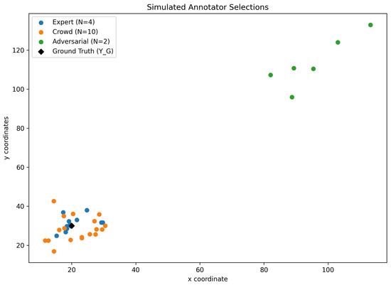
Figure 1.
Simulated annotations. Simulated annotations for the toy problem, demonstrating the selections for the expert, crowd-sourced and adversarial groups, as well as the canonical ground truth .
- Annotator a is a member of one of the three groups (g): expert, crowd and adversarial;
- to is the range of offset integers available for random selection in both x and y directions for the corresponding group g;
- is a random sample from a normal distribution with mean 0 and standard deviation 1.
As each annotator identified the landmark multiple times, additional variance for each selection (see Equation (5)) was generated by selecting random values for each annotator’s standard deviation, again representative of effort and skill: , and , and combining them with each of the normally generated random values :
where:
- Annotator a is a member of one of the three groups (g): expert, crowd and adversarial;
- to is the range of standard deviation values available for random selection in both x and y directions;
- is a sample from a normal distribution with mean 0 and standard deviation 1.
Finally, the two components were combined to generate the entire annotation set by randomly applying a sign to to ensure that the annotator’s selections were not consistently to one side of .
where:
- is the annotation set for annotator a;
- is a random sign selection of −1 or 1.
With the simulation annotation set created, the landmark derivation method of Algorithm 1 was applied to the expert data, expert + crowd data and finally all examples to determine the approximation of the ground truth location ( and ) as well as determine if any benefit could be attributed to the groups alone. Each location was then compared with the value of the global mean using the Euclidean distance from . This is one major advantage of using simulated annotations in the toy problem as, unlike some real-world annotations tasks, the canonical ground truth landmarks are known and available, thus providing an objective means of assessing the performance of the proposed method.
To determine if the proposed method is sensitive to any of the randomly selected parameters, a second iteration of the toy problem was executed with a different set of randomly selected parameters. For the second iteration, a distribution of , and annotators was selected, with each group identifying the same landmark times. A canonical ground truth landmark of was randomly selected, as well as non-zero mean noise values of , and . A second set of values representing annotator effort and skill was also randomly selected as and .
The source code that was used to run this analysis is available via github [14].
3.2. Facial Landmark Experimentation
In the second experimental component, we completed an experimental study of facial landmarks identified by expert and crowd-sourced annotators on a variety of images using Amazon Mechanical Turk. During this study, we presented crowd-sourced and expert annotators with a random sequence of four different images. In accordance with the experimental framework described above, there was expected to be some component of adversarial annotators; however, their representation could not be determined prior to the study. It was assumed that the adversarial annotators would be present as some component of the group, if they were present at all. The images, as shown in Figure 2, were selected from both the 300W [15] and MUCT [16] datasets as they contain a variety of expressions, poses, lighting and environments.
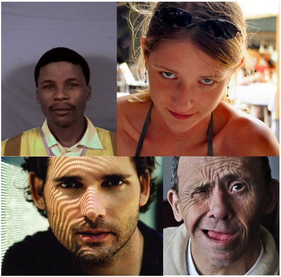
Figure 2.
Images selected for annotation. These images were selected for manual landmark annotation. The image in the top left corner was sourced from MUCT [16], and the remainder were sourced from the 300W dataset [15].
The annotators were asked to identify 22 separate landmarks on each image, and were shown each image times. To avoid bias, the order of the landmarks to be annotated was randomised for each image presentation, where the annotator was shown an example image of the current landmark to be identified (such as those shown in Figure 3). While the annotators were sourced from the Mechanical Turk system, the expert annotators were recruited from within our research group given their previous experience in the task.
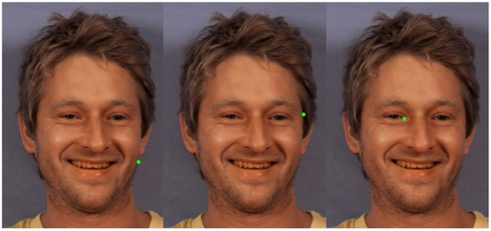
Figure 3.
Example landmarks. A sample of images used to indicate the current landmark to be identified.
In contrast to the previous toy problem, there is no known canonical landmarks available for the experimental study. The exact location of facial landmarks selected on images is subjective. While some landmarks may be categorised as clearly inaccurate, e.g., the tip of the ear is identified instead of the corner of the eye, in some situations, it is impossible to say that one annotator’s interpretation is better than another. Because of this, unlike the toy problem where an empirical comparison could be made, the locations of the derived and mean landmarks in this experimental study were visually assessed and their final positions were compared. By comparing the location of the derived and mean landmarks, the overall effect of Algorithm 1 compared with considering the performance of all annotators to be equal could be determined.
4. Results
4.1. Toy Problem
The simulated landmarks generated for each of the annotator groups in the toy problem, as well as the location of the canonical ground truth, can be seen in Figure 1. Intuitively, it can be seen that the expert group is consistently closer to than the crowd-sourced and adversarial groups. Figure 4 shows the location of the annotated positions with respect to the canonical location, global mean () and derived ground truth locations (). The dotted line in each plot shows the trajectory taken by the derived locations over each iteration of the method.
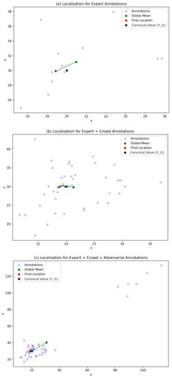
Figure 4.
Toy problem ground truth localisation. This plot shows the final location of the proposed method for the desired groups compared to the canonical ground truth and the global mean. The dotted line shows the path taken by over each iteration to its final location. Figure (a) shows the results for the expert group only, (b) the expert + crowd groups and (c) all simulated data.
Table 1 shows the Euclidean distance of the global mean and derived locations from the canonical ground truth. For the first iteration of the toy problem, the final position as determined by Algorithm 1 in all three examples was , where and the global mean . As such, the Euclidean distance is significantly less than the difference between the global mean and ground truth value .

Table 1.
Euclidean distance from . This table contains the Euclidean distance of each localisation method for each dataset to , in pixels.
For the second iteration of the toy problem , the proposed method produced position estimates of for the expert group alone and when including the remaining groups. The Euclidean distances are shown in Table 1.
4.2. Facial Landmark Selection
Figure 5 shows the individual facial landmark selections as collected from the expert and crowd-sourced annotators, including replicates. These point clouds demonstrate the extent of variability and uncertainty in identifying each of the landmarks. This is particularly evident when inspecting the landmarks that lie on the border of the face, as it can be seen that the annotators correctly associate the position with the facial edge but have trouble identifying exactly where on the border the points belong to. Figure 6 compares the location of the global mean for each landmark with that selected using our iterative method. Similarly to the results shown within the toy problem section, this image indicates the initial global mean positions with a green cross. The final ground truth landmark positions found using our method are also shown in the images as a red cross. The path followed from the initial seed position to the final position is indicated by the dotted lines within the images.
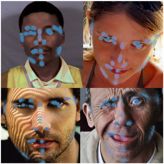
Figure 5.
Individual ground truth localisation. This plot shows the location of the individual landmarks selected by the annotators.
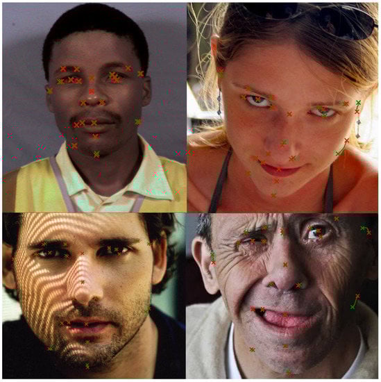
Figure 6.
Facial landmark ground truth localisation. This plot shows the location of the mean landmark location (shown in green) as well as the derived ground truth (red crosses). The lines joining the green and red crosses show the path taken from the initial mean location to the derived ground truth location.
5. Discussion
As discussed in the Introduction section, one of the key challenges met during this study was how to select ground truth landmark positions in problems of high subjectivity, where it may not be possible to determine a ‘true location’. How can one position be right or wrong if the selection is a matter of opinion? This was one of the key drivers for the use of the toy problem in this study, as it provides a mechanism for delivering a single correct location while also representing the performance of each annotator. The synthetic data are a very close approximation to producing a globally known and agreed upon ground truth landmark in a regression problem. As such, these data provide a mechanism for objectively comparing our method of landmark selection with that of the global mean. As shown in Table 1, for each group of annotators—expert, crowd and adversarial—the proposed method was able to estimate the ground truth location with a greater accuracy than computing the global mean in both iterations of the toy problem. Other than achieving an improved performance, the method also demonstrated a degree of robustness to differing the parameter selection as shown by the second iteration of the toy problem. This is further supported by the path of the landmark estimate through each of the iterations as shown in Figure 4, for each of the annotator groups, on each iteration tracking towards the simulated ground truth position and finally residing closer to the final ’known’ position.
When applying our method of landmark determination to a set of actual annotations, we can again see an improvement in the final position location comparing Figure 5 and Figure 6 to the instructed positions in Figure 3. In comparison with the toy problem, an overall objective position cannot be objectively determined due to the subjective nature of the task; however, by visually comparing the final selected positions, shown by the red crosses in Figure 6, we can see improvements in the final selections. Landmarks around the border of the face and eyes are more accurately positioned on the boundaries, while positions with strong locating features such as the corner eyes exhibit less improvement. Two particularly effective examples are shown by the two images on the right of Figure 6 as they provide examples with extreme facial expressions as well as poses in the image.
It is also interesting to note that the proposed method is invariant to the order in which the annotations are presented due to the use of the global mean as the starting position seed. With the same starting position, the iterative loop will always compute the same precision for each annotator and thus will eliminate annotators in the same order. This is the only time in the process where all annotators are considered equal and it ensures that the process is repeatable. Using seed positions that vary for each execution may result in different starting locations of and thus could lead to differing outcomes. Further study would be required to determine if this would lead to improved results or not.
When considering if the annotator precision method of ground truth derivation is suitable, it would be beneficial for the reader to assess or estimate the intra-annotator variance for each landmark of interest. One of the primary advantages of the proposed method is the ability to weight more accurate annotators higher in determining the final position, even when all of the annotators are considered ‘experts’. In situations where each of the annotators are comparable in performance, the additional complexity of this method may not be worthwhile; such as the results produced by the toy problem.
While this work featured numerous examples of facial landmarking as regression problems, the application of the proposed method is certainly not limited to these types of problems. It is expected that this method could be used in many different problems with manually annotated co-ordinates in datasets, such as identifying locations or positions on a map, or point clouds to define an abstract geometry.
Potential Future Research
In this paper, we describe a method that considers the precision of each individual annotator for each landmark separately, thus allowing the best annotators to be used to determine the optimal location of individual landmarks. One aspect of the described method is that the iterative annotator precision computation/annotator removal process repeats until the final and most precise annotator remains to form the final landmark selection. While not included within this article, a number of modifications may be further studied to improve the final result.
- The termination of the iterative loop: throughout this study, we removed the least precise annotator on each iteration until only one annotator remained. In datasets where there is a high level of disagreement between annotators, the termination criteria could be adjusted to try and improve the overall result, e.g., terminating the iteration when two or three annotators remain. Such an adjustment could allow for underperforming annotators to be removed while allowing for a degree of consensus amongst the higher performing. Other means of termination also include stopping when the derived landmark position stops moving within a defined amount.
- Different stating position seeds: in this study, we used the global mean position for each landmark as the initial seed to determine annotator precision. Other seeding methods may also be useful for further study, such as using the expert annotator’s mean selection or randomly selecting one selected landmark location and repeating Algorithm 1 multiple times.
- A weighted averaged based on annotator precision was specifically selected as the update mechanism, as higher-performing annotators contribute more to the overall result. The effect/impact of alternative update mechanisms could be investigated.
6. Conclusions
In conclusion, we propose a novel method for deriving precise ground truth labels for regression problems based on the performance of individual annotators separately for individual co-ordinates. This method provides more robust final values, even in situations where canonical ground truth positions cannot be determined. We have presented this method with experimental results from a simulated toy problem that provides an objective means for demonstrating the improved performance. There is potential for further study and improvement by investigating different termination or seed conditions as well as different methods for weighting annotator precision. In this study, we also employed a novel method to demonstrate the improved performance using crowd-sourced labels for an image-based facial landmarking problem.
Author Contributions
Conceptualization, B.J.; Methodology, B.J.; Software, B.J.; Validation, B.J.; Data curation, B.J.; Writing—original draft, B.J.; Writing—review & editing, P.d.C.; Supervision, P.d.C. All authors have read and agreed to the published version of the manuscript.
Funding
This research received no external funding.
Institutional Review Board Statement
Not applicable.
Informed Consent Statement
Not applicable.
Data Availability Statement
The source code of the method described, as well as the experimental data, can be found at https://github.com/doc-E-brown/johnstondechazal (accessed on 5 August 2023).
Conflicts of Interest
The authors declare no conflict of interest.
Abbreviations
The following abbreviations are used in this manuscript:
| SDB | Sleep-Disordered Breathing |
| MLE | Maximum Likelihood Estimation |
References
- Balaei, A.T.; Sutherland, K.; Cistulli, P.A.; de Chazal, P. Automatic detection of obstructive sleep apnea using facial images. In Proceedings of the 2017 IEEE 14th International Symposium on Biomedical Imaging (ISBI 2017), Melbourne, VIC, Australia, 18–21 April 2017; pp. 215–218. [Google Scholar] [CrossRef]
- Johnston, B.; de Chazal, P. Automatic PAP Mask Sizing with an Error Correcting Autoencoder. In Proceedings of the 2019 41st Annual International Conference of the IEEE Engineering in Medicine and Biology Society (EMBC), Berlin, Germany, 23–27 July 2019; pp. 3677–3680. [Google Scholar] [CrossRef]
- Johnston, B.; de Chazal, P. A Fully Automated System for Sizing Nasal PAP Masks Using Facial Photographs. In Proceedings of the 2018 40th Annual International Conference of the IEEE Engineering in Medicine and Biology Society (EMBC), Honolulu, HI, USA, 18–21 July 2018; pp. 3979–3982. [Google Scholar] [CrossRef]
- Guarin, D.L.; Yunusova, Y.; Taati, B.; Dusseldorp, J.R.; Mohan, S.; Tavares, J.; van Veen, M.M.; Fortier, E.; Hadlock, T.A.; Jowett, N. Toward an Automatic System for Computer-Aided Assessment in Facial Palsy. Facial Plast. Surg. Aesthetic Med. 2020, 22, 42–49. [Google Scholar] [CrossRef] [PubMed]
- Aryal, A.; Becerik-Gerber, B. Skin Temperature Extraction Using Facial Landmark Detection and Thermal Imaging for Comfort Assessment. In Proceedings of the 6th ACM International Conference on Systems for Energy-Efficient Buildings, Cities, and Transportation, New York, NY, USA, 13–14 November 2019; ACM: New York, NY, USA, 2019; pp. 71–80. [Google Scholar] [CrossRef]
- Raykar, V.C.; Yu, S.; Zhao, L.H.; Valadez, G.H.; Florin, C.; Bogoni, L.; Moy, L. Learning from crowds. J. Mach. Learn. Res. 2010, 11, 1297–1322. [Google Scholar]
- What Is CAPTCHA? Available online: https://support.google.com/a/answer/1217728 (accessed on 9 July 2023).
- Dzieza, J.T.V. Why CAPTCHAs have gotten so difficult. The Verge, 1 February 2019. [Google Scholar]
- Johnston, B.; de Chazal, P. A review of image-based automatic facial landmark identification techniques. Eurasip J. Image Video Process. 2018, 2018, 86. [Google Scholar] [CrossRef]
- Dawid, A.P.; Skene, A.M. Maximum Likelihood Estimation of Observer Error-Rates Using the EM Algorithm. Appl. Stat. 1979, 28, 20. [Google Scholar] [CrossRef]
- Seah, J.C.Y.; Tang, C.H.M.; Buchlak, Q.D.; Holt, X.G.; Wardman, J.B.; Aimoldin, A.; Esmaili, N.; Ahmad, H.; Pham, H.; Lambert, J.F.; et al. Effect of a comprehensive deep-learning model on the accuracy of chest x-ray interpretation by radiologists: A retrospective, multireader multicase study. Lancet (Br. Ed.) 2021, 3, e496–e506. [Google Scholar] [CrossRef]
- Sinha, V.B.; Rao, S.; Balasubramanian, V.N. Fast Dawid-Skene: A Fast Vote Aggregation Scheme for Sentiment Classification. arXiv 2018, arXiv:1803.02781. [Google Scholar]
- Johnston, B.; de Chazal, P. The Effect of Landmark Variability on Automated PAP Mask Sizing. In Proceedings of the 2019 41st Annual International Conference of the IEEE Engineering in Medicine and Biology Society (EMBC), Berlin, Germany, 23–27 July 2019; pp. 4129–4132. [Google Scholar] [CrossRef]
- Python Implementation. Available online: https://github.com/doc-E-brown/johnstondechazal (accessed on 21 May 2023).
- Sagonas, C.; Antonakos, E.; Tzimiropoulos, G.; Zafeiriou, S.; Pantic, M. 300 Faces In-The-Wild Challenge: Database and results. Image Vis. Comput. 2016, 47, 3–18. [Google Scholar] [CrossRef]
- Milborrow, S.; Morkel, J.; Nicolls, F. The MUCT Landmarked Face Database. Pattern Recognition Association of South Africa. 2010. Available online: http://www.milbo.org/muct/The-MUCT-Landmarked-Face-Database.pdf (accessed on 5 August 2023).
Disclaimer/Publisher’s Note: The statements, opinions and data contained in all publications are solely those of the individual author(s) and contributor(s) and not of MDPI and/or the editor(s). MDPI and/or the editor(s) disclaim responsibility for any injury to people or property resulting from any ideas, methods, instructions or products referred to in the content. |
© 2023 by the authors. Licensee MDPI, Basel, Switzerland. This article is an open access article distributed under the terms and conditions of the Creative Commons Attribution (CC BY) license (https://creativecommons.org/licenses/by/4.0/).