Article

Current Limitations for Predicting Liquid Dispersion in Continuous Flow Bubble Columns Using CFD

by
Juan José Gallardo-Rodríguez
1,2,*,
Javier Velasco-Amate
1,
Erika Lorenzo-Horcajo
1,
Lorenzo López-Rosales
1,2,
Yusuf Chisti
3,
Francine Battaglia
4,
Asterio Sánchez-Mirón
1,2 and
Francisco García-Camacho
1,2
1
Department of Chemical Engineering, University of Almería, 04120 Almería, Spain
2
Research Center CIAMBITAL, University of Almería, 04120 Almería, Spain
3
Institute of Tropical Aquaculture and Fisheries, Universiti Malaysia Terengganu, Kuala Nerus 21030, Terengganu, Malaysia
4
Department of Mechanical and Aerospace Engineering, University at Buffalo, Buffalo, NY 14260, USA
*
Author to whom correspondence should be addressed.
Appl. Sci. 2023, 13(16), 9250; https://doi.org/10.3390/app13169250
Submission received: 25 July 2023 / Revised: 11 August 2023 / Accepted: 13 August 2023 / Published: 15 August 2023
(This article belongs to the Section Applied Biosciences and Bioengineering)

Abstract

:
Liquid-phase dispersion in a continuous flow bubble column was studied using computational fluid dynamics (CFD) and different combinations of turbulence and biphasic models. The results were compared with the experimental data obtained by the stimulus-response method in an air-water pilot-scale bubble column (2 m tall, 0.234 m internal diameter). Two flow combinations were examined: high flow rates of 3.2 m3 h−1 and 4.5 m3 h−1 and low flow rates of 1.98 m3 h−1 and 0.954 m3 h−1 for water and air, respectively. The objective was to evaluate commercial CFD 16.1 software to predict flow behavior beyond macroscale parameters such as hold-up or mixing time. The turbulence models that best replicated the experimental tracer dispersion were large eddy simulation-type models: scale-adaptive simulation (SAS) and shear stress transport-SAS. The simulations qualitatively predicted the tracer concentration with time but were unable to reveal the small-scale perturbations in the biphasic system. The predicted tracer residence time was double or triple the measured times for low and high flow, respectively.

1. Introduction

A bubble column is typically a vertical cylindrical vessel with a continuous liquid phase and a dispersed gas phase. Bubble columns are widely used for gas-liquid reactions because of their simplicity and ability to achieve good interphase mass transfer [1,2,3]. Geometric factors (column diameter and height, features of the gas sparger), the properties of fluids, and flow rates of the gas and liquid phases influence important operational characteristics such as gas holdup (volume fraction of gas in gas-liquid dispersion) and gas-liquid interfacial area for mass transfer in bubble columns [1,2,3,4,5]. Although simple in geometric configuration, bubble columns are characterized by a complex two-phase flow [6,7]. The flow in a bubble column is influenced by the movement of the gas bubbles, which in turn depends on their size and size distribution and on gas holdup [8]. The random movement of bubbles, bubble coalescence and breakup, and interaction with the column walls, create complex turbulence patterns that can be difficult to predict.
Different flow regimes and extents of backmixing (mixing along the axial direction) are desirable in bubble columns for different applications [9]. Some processes require high superficial velocities of phases to achieve a highly turbulent heterogenous flow regime to support the required rates of mass transfer and reaction [10,11,12]. In other cases, much lower flow velocities are satisfactory and actually desired to minimize the energy input and the turbulence-associated damage to biological systems [13].
Different aspects of the performance of a bubble column are characterized in terms of gas holdup, the axial and radial liquid-phase dispersion coefficients, and gas-liquid volumetric mass transfer coefficients [1,2,3,5]. Many empirical correlations have been developed for estimating these performance characteristics in different media and flow regimes [1,2,3,5,14].
The mixing caused by the convective motion of fluids in a bubble column has axial and radial components. Axial and radial dispersion coefficients are used to characterize this mixing. The dispersion coefficients are analogous to the diffusion coefficients of Fick’s law [15]. In bubble columns operated batchwise with respect to the liquid phase, mixing is often characterized in terms of a mixing time, or the time required to achieve a specified deviation (e.g., 5%) from the state of complete mixedness (equilibrium concentration) after the injection of a tracer [16]. Continuous-flow bubble columns are characterized by the transient response of the tracer concentration [17].
Computational fluid dynamics (CFD) provides a valuable tool for describing local physical phenomena encountered in bubble column flows and, therefore, quantitatively predicting the behavior of the phases [18]. Accurate predictions are possible by using direct numerical simulation (DNS) instead of simplifying models, but this would require supercomputing facilities, especially for large columns [19].
Although computationally demanding in terms of hardware power, biphasic models based on Euler–Lagrange (E-L), such as volume of fluid (VOF), provide a clear physical description of particle movement (e.g., gas bubble), or fluid flow, and therefore are expected to become the norm in modeling flow in the future as more powerful computers become more readily accessible. At present, because of the computational demands of E-L models, studies based on them have been limited to small-sized equipment that is not particularly relevant to large-scale industrial operations. Therefore, most of the current two-phase CFD studies have used Euler–Euler (E-E) modeling schemes [20]. The VOF model and the E-E two-fluid model are very different models. In the VOF model, a single flow field is used to describe the two phases and solve a single set of flow and energy equations. Interfacial forces exist in the interface layer and act as a source term in the Navier–Stokes (N-S) equations (only one vector equation for the two-phase flow). The mesh size for VOF models must be sufficiently small so that a smooth interface can be constructed for the bubble. In the E-E model, the dispersed phase is treated as a virtual continuous fluid. As a consequence, one set of N-S equations is needed for each phase to separately describe the virtual continuous fluid and the real continuous fluid. Both fluids occupy the whole space. Interaction forces between the two fluids are needed to connect them.
Numerous CFD simulations of the air–water system in bubble columns have been reported, showing acceptable predictions of the average magnitudes of the fluid dynamics and mass transfer parameters [12,21,22,23]. The majority of them, especially for pilot-scale systems, have been conducted using Reynolds-averaged Navier–Stokes (RANS) models. RANS models (e.g., kinetic energy-dissipation rate (k-ε) turbulent model) and large eddy simulation (LES) models have been compared for describing flow in a rectangular bubble column [24]. RANS models overestimated the turbulent viscosity and were unable to provide estimation in the sparger area. LES, on the other hand, allowed better predictions of both flow and turbulent viscosity [24]. RANS models have been shown to overestimate the size of the bubbles, and better estimates are obtained using the renormalization group (RNG) methods [25]. The bubble size is of critical importance in bubble columns as it affects the coalescence and breakup of bubbles and also the gas-liquid interfacial area for mass transfer. If bubble coalescence and breakup are poorly modeled, the simulated flow pattern deviates from the actual one [25,26].
Transient three-dimensional LES of a bubble column for a wide range of gas velocities best predicted the flow pattern of bubble plumes [26]. A comparison of the predictive performance of different turbulence models (k-ε, k-ω, RNG, Reynolds stress model (RSM), and LES) showed that the RSM predictions of liquid velocities, gas holdup, and energy dissipation rates were comparable to the LES results but required less computational time [27]. RSM models can account for flow instabilities while maintaining good predictions of average magnitudes and computational economy [22]. A combination of the baseline model (k-ω for walls and k-ε for the other domains) with the explicit algebraic Reynolds stress model (EARSM) has been found to be effective in the simulation of flow fields and local turbulence [22].
The use of LES in relation to dispersed bubble flows has been comprehensively reviewed [20]. A failure to correctly select values for key parameters (e.g., time-step, total time, grid size, etc.) limits the performance of LES. Although LES is conceptually simple, its application is not because several parameters need to be specified and their selection is not straightforward. LES predictions have agreed well with experimental data, mainly at low values of superficial gas velocities and gas holdups [20]. This is thought to be caused by the limitations of E-E schemes for representing interphase forces and bubble-induced turbulence [28]. Simulations of a large bubble column using an E-E approach (k-ε turbulence model with an additional term for bubble turbulence) achieved good predictions of the phase velocities and mixing times [29,30], but the model overpredicted the local holdup, particularly in the center of the column.
Although for batch bubble columns several CFD models have been studied, liquid-phase dispersion in two-phase continuous-flow bubble columns has not been previously examined using CFD. Therefore, the present study focused on the use of CFD to characterize mixing in a large bubble column with continuous flows of the phases (air and water). Two sets of conditions combining high and low flows were assessed by simulations and experiments. The volume of fluid (VOF) scheme and turbulence models (RANS and LES) available in ANSYS Fluent® (Canonsburg, PA, USA) were evaluated for their predictive performance and compared with the experimental data of a liquid tracer dispersion.

2. Materials and Methods

2.1. Validation Experiments

Mixing experiments for water and air were analyzed in a cylindrical column (height = 2 m; internal diameter = 0.234 m) made of clear poly(methyl methacrylate) (Figure 1). The operating temperature was 20 °C, the pressure above the column was 1 atm, and the volume of water in the column was 0.086 m3. Mixing characteristics were measured using the tracer-response method [31]. Water flow (up flow) was first established (Qw = 1.98 or 3.18 m3 h−1) and then the air flow was turned on (Qa = 0.954 or 4.5 m3 h−1). Re were 3 and 4.8 × 10³ for the low and high flows, respectively. Deionized water, free of all carbonaceous species [32], entered the column from a storage tank via a centrifugal pump. The water entering the column was uniformly distributed over its cross section by means of a poly(vinyl chloride) (PVC) plastic distributor (41 holes of 8 mm diameter; total hole areas for liquid flow = 2.06 × 10⁻³ m2) (Figure 1). A cross-pipe PVC air sparger (36 holes, 1 mm in diameter, total hole area for air flow = 2.83 × 10⁻⁵ m2) was located just about the liquid distributor (Figure 1). The fluids exited the column at the top through 5 outlet tubes (27.5 mm diameter, total hole area = 2.97 × 10⁻³ m2) (Figure 1). The large outlet holes minimized the pressure drop, and the column operated at atmospheric pressures.
Each tracer pulse consisted of 40 mL of 37% hydrochloric acid. Tracer was injected into the inlet water pipe via a syringe (Figure 1). The pH was monitored with four electrodes placed at different axial and radial positions in the column. Two pH electrodes were positioned 1.05 m above the base of the column, and another two electrodes were located 1.84 m above the base. The electrodes entered the column at an angle of 45° to the horizontal. At any axial location, the tip of one of the electrodes was coincident with the centerline of the column (r = 0 m), whereas the second electrode had its measuring tip located at a radial distance r of 0.1 m from the centerline of the column. Data from the pH sensors (Crison Instruments, Alella, Spain, model 53 33) were recorded with a LabJack data acquisition card connected to a laptop PC via USB port (1 s sampling rate).

2.2. CFD Simulations

The numerical simulations were performed using ANSYS Fluent® 16.2 software (Ansys, Inc., Canonsburg, PA, USA) on an HP Z840 workstation (HP Inc., Palo Alto, CA, USA) with two Intel® Xeon® CPU E5-2670 v3 2.30 GHz processors and 128 GB of RAM. ANSYS Fluent uses the fundamental governing equations of fluid dynamics, which include the continuity equation, Navier-Stokes equations for momentum, and the energy equation (for compressible flows). ANSYS DesignModeler® was used for the 3D drawing of the bubble column. The CutCell (ANSYS Meshing®) assembly method was employed to obtain a mesh aligned with the flow direction. Several meshes were compared. They were generated by increasing the number of cells and using the “inflation” method of decreasing the size of cells in the direction normal to the wall. The result was a finer mesh near the wall. Details of the meshes are provided in the Supplementary Materials (Table S1). Grid-independent meshes were obtained for each scheme by observing the velocity profiles for air and water. For RANS models (using k-ε and E-E), the mesh had 3.9 × 10⁵ cells (maximum size 3.2 × 10⁻² m). For LES models (using scale-adaptive simulation, SAS, and VOF), the mesh had 6.9 × 10⁵ cells (maximum size 1.6 × 10⁻² m). Convergence was checked by comparing the residual at an iteration of a timestep with the residual at the beginning of the timestep (residuals below 10−5).
The turbulence models included the standard k-ε, realizable k-ε, RNG k-ε, SST, SAS detached eddy simulation (DES), and LES. Default configurations of the turbulence models in Fluent were used in the simulations. The turbulence models and the solution methods (discretization) are summarized in Table 1. Several turbulence models included in ANSYS Fluent® were first compared for tracer dispersion in single-phase water flow (no air sparging). Achieving a uniform tracer distribution through all the holes of the liquid distributor was essentially impossible; therefore, tracer injection was simulated exactly as in the validation experiments. The physical properties of fluids have been included in Table 2. The tracer inlet was included within the liquid inlet tube (Figure 1A). The inlet was defined as a mass flow inlet with a constant mole fraction of H+ (tracer) depending on the pH of the inlet water. The duration (ti) of the tracer injection pulse was 2.5 s, and the hydrochloric acid tracer injected had a H+ mole fraction (xi) of 0.2246 (Table 3).
The tracer concentration was monitored in several positions by defining point surfaces at the locations where the pH electrodes were situated and monitoring these surfaces. Data for every time step was saved (t = 0.01 s).
For the two-phase flow study, two experimental conditions with different extreme flow rates of water and air were simulated (Table 3). The air sparger was also defined as a mass flow inlet. The column outlet was defined as a constant atmospheric pressure outlet (1 atm), and no-slip conditions were assumed at the walls. The superficial velocities of air (ua) and water (uw) were calculated based on the cross-sectional area of the column. Convergence was assumed if the residuals were smaller than 10−5 at each time step.

3. Results

3.1. Velocity Profiles for Mono- and Biphasic Simulations

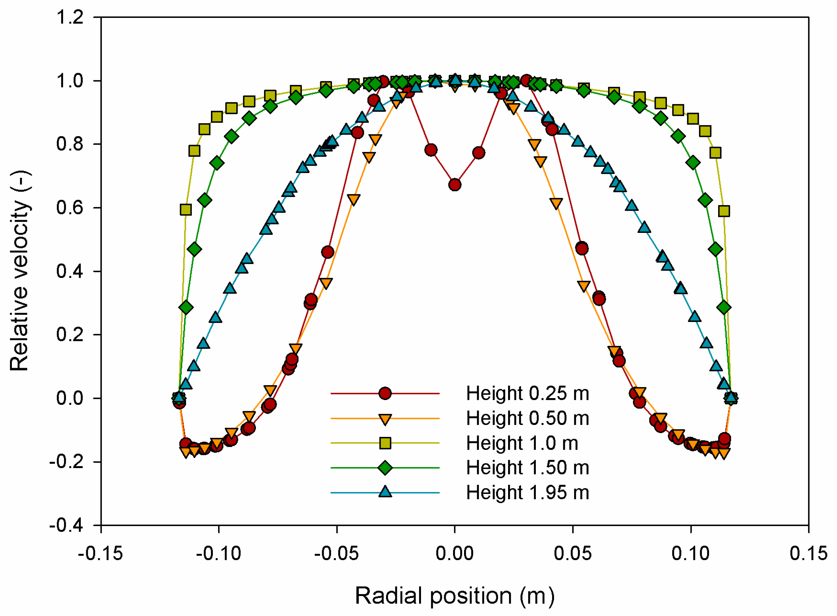
CFD predictions of the relative water velocities (relative to the maximum value at the specified height of the column) as functions of radial position are shown in Figure 2 for a single-phase flow of water. The simulations used the k-ε turbulence model and an imposed water flow rate (Qw) of 1.98 m3·h1. The computed velocity profiles depended on the mesh size used for the simulations (Supplementary Materials, Figure S1), especially in the lower entry region of the column. As was expected, biphasic simulations required finer meshes. Except in the vicinity of the column inlet, the radial velocity profiles had a parabolic shape consistent with expectations [25]. The flow velocity was maximum at the centerline of the column and minimum at the walls (Figure 2). The sole exception was the M-shaped radial velocity profile at a column height of 0.25 m (Figure 2). This shape was due to velocity distortions associated with the location of the liquid distributor below the air sparger (Figure 1A). Although there was no flow of gas, the liquid lost velocity as it impacted the sparger. The M-shaped profile was essentially an entrance effect that disappeared above 0.5 m (Figure 2). Over a column height of 1.0–1.5 m, the radial velocity profile had a plug-flow character and had not fully developed into the parabolic profile seen at a column height of 1.95 m (Figure 2).
The parabolic shape of the profile (noticeably higher flow at the centerline than elsewhere) close to the outlet (column height of 1.95 m; Figure 2) was also contributed by the end effect of the flow exit tubes near the top of the column: more flow exited through the central tube compared to the peripheral ones. The negative relative velocities close to the walls (Figure 2) indicated downflow or recirculation of the liquid. The cause of the recirculation was a significant resistance to flow at the outlet tubes near the top of the column. As the flow could not exit through the entire cross section of the column because of the narrowing of the cross section into the exit tubes (Figure 1A), some of the flow descended near the walls. The relative radial velocity profiles predicted for air (Qa = 0.954 m3·h1) and water (Qw = 1.98 m3·h1) in two-phase flow are shown in Figure 3. The gas phase was simulated using the dispersed Eulerian two-phase model. The radial velocity profiles (Figure 3) were markedly different compared to the profiles observed for single-phase water flow (Figure 2). The two-phase profiles had a relatively sharp peak in the central axial region, indicating a substantially faster flow of both phases in the core zone of the column compared to the flow in the peripheral zone of the cross section (Figure 3).
The central region velocity peaks were sharper near the base of the column (height = 0.25 m; Figure 3). Although these peaks broadened as the flow moved up the column, they persisted throughout the entire height (Figure 3). The reason for the faster flow in the core zone was an entry effect: both fluids entered at the base of the column in the central regions, and therefore the velocity in this zone was the highest. Closer to the exit of the column (1.95 m from the base), the core zone velocity showed a noticeable increase (Figure 3) due to preferential flow through the central outlet tubes at the top. The high core flow may be partly attributable to the fact that the rapidly rising larger bubbles concentrated in the center of the column [33]. These bubbles entrained liquid in their wake, which increased the liquid velocity in the core zone. Peripheral regions outside the core zone had more uniform bubble distributions over the column cross section. A nonuniform radial distribution of gas in bubble columns has also been reported in bubble columns operated batchwise with respect to the liquid phase [26].

3.2. Liquid Phase Dispersion in Single-Phase Water Flow

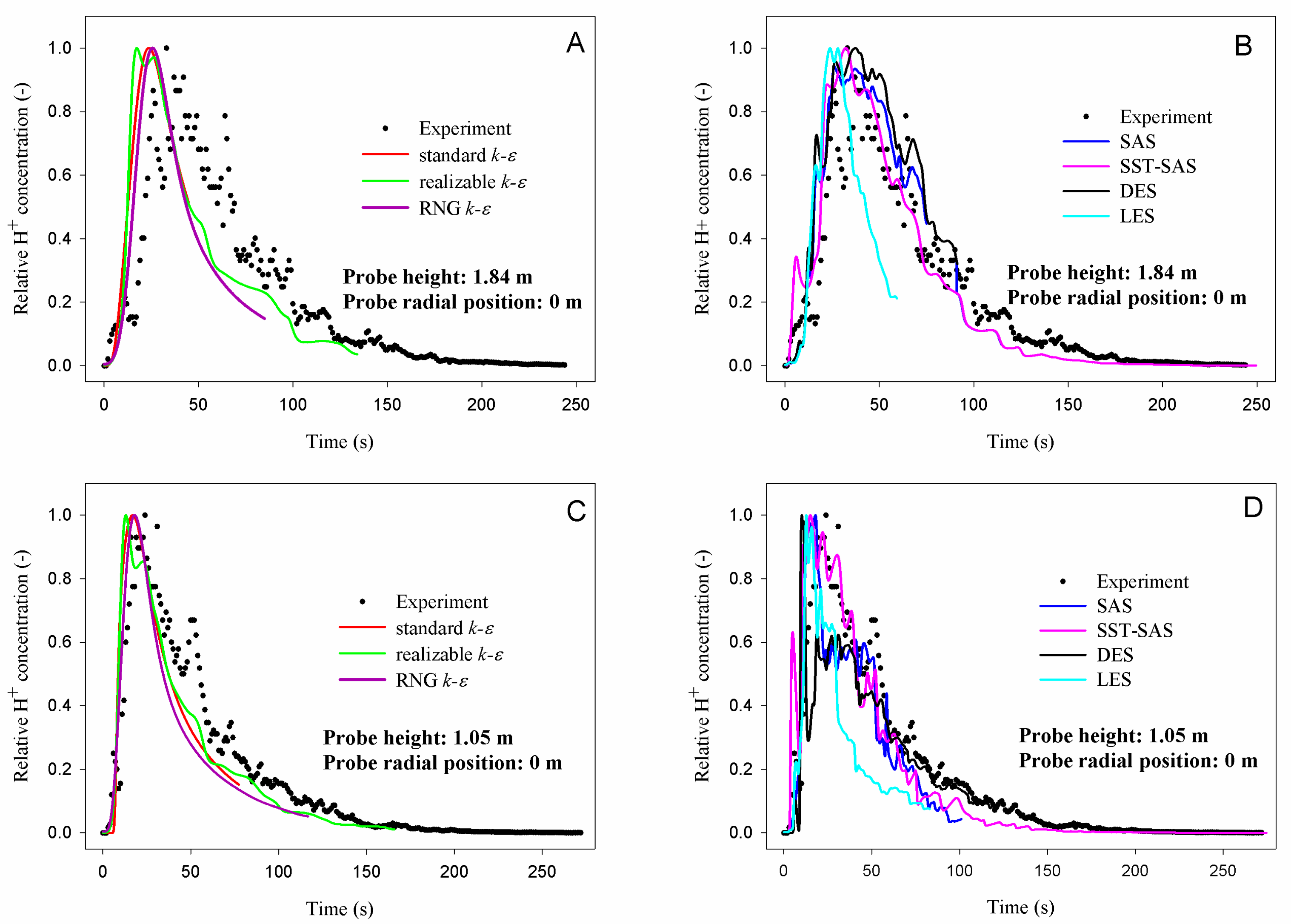
First, CFD simulations were performed to identify the turbulence model that best predicted the experimental tracer dispersion in the single-phase water flow. The flow rate of water was fixed at the highest setting (Qw = 3.2 m3·h1, Re = 4.8 × 10³). The temporal evolution of the CFD and experiment tracer responses was compared (Figure 4), corresponding to the centerline (r = 0 m) of the column at two different axial positions (z = 1.05 and 1.84 m). Although no single uncertainty estimate can be attributed to a pH measurement procedure, it has been shown that the pH measurement uncertainty for commercial glass electrodes is less than 0.05 pH units [34]. All data in Figure 4 were normalized using the highest measurement within a set for ease of comparison. Thus, the relative concentration of the tracer ranged between 0 and 1 (Figure 4). The experimental and simulated tracer responses at both axial positions followed a typical stimulus-response pattern characteristic of concurrent continuous flow: the tracer concentration rose rapidly to a peak value and then declined slowly to an equilibrium value.
The standard, realizable, and RNG k-ε turbulence models reproduced the general trend but not the instabilities of tracer concentration (Figure 4A–C). In general, the three RANS models differed a little in their responses, for example, in their predictions of the time for the tracer to reach the measurement points. The model that best reproduced the trace peak width was the realizable k-ε model. As these are averaged models, they are not capable of capturing the finer details of the tracer response spectrum [20].
Secondary peaks were observed between 50 and 100 s on the time axis (Figure 4) because of the previously mentioned recirculation zones near the walls. The secondary peaks were only correctly captured by SAS and SST-SAS (Figure 4B–D). The SAS model predicted a somewhat narrower peak at the lower probe location (z = 1.05 m) compared to experimental data but adjusted well to the peak width at the higher probe location (z = 1.84 m; Figure 4B) and also predicted well the time to reach the maximum tracer concentration.
The problem with the SST model was that for both axial positions (z = 1.05 and 1.84 m), the tracer reached the measurement points quickly and also left these points rapidly (hence the narrow-predicted peaks) (Figure 4B–D). Overall, the SAS model and the SST-SAS model best reproduced the experimental responses, including some perturbation details, including the small secondary peak before the maximum tracer concentration.

3.3. Liquid-Phase Dispersion in Air-Water Two-Phase System

Two-phase flow in bubble columns has highly turbulent and anisotropic characteristics [25]. For batch bubble columns, it has been shown that RANS models are suitable for simulating flow when the objective is to obtain a stationary solution and the usual assumption of isotropic turbulence applies. The two-phase systems in bubble columns do not conform to the isotropic turbulence requirement because of the bubbles. In addition, the pulse tracer mixing processes are transient, and therefore the use of RANS models for such systems requires caution [26]. Therefore, for the continuous bubble column, based on the liquid-single-phase dispersion study, the SAS and SST-SAS models were selected for simulating the air-water (two-phase) system.
It was found that stable two-phase simulations could not be performed using the SST-SAS model as the solution diverged after a few time steps, irrespective of the time step and the under-relaxation coefficients. Although the SST is a comprehensive model, instabilities develop, resulting in divergence issues in complex flows [20]. Therefore, the SAS turbulence model was adopted, as it had also demonstrated a good fit to the experimental data (Figure 4B–D). In Fluent® (Canonsburg, PA, USA), only the VOF two-phase model is compatible with the SAS turbulence model and requires surface tension for accurate simulations [28]. Both the low (Qw = 1.98 m3 h−1, Qa = 0.954 m3 h−1) and high flow (Qw = 3.2 m3 h−1, Qa = 4.5 m3 h−1) scenarios were simulated using SAS-VOF.
Compared to other LES approaches, SAS considers the ratio of the turbulent length scale to the von Karman length scale as a dimensionless measure of non-homogeneity. Therefore, the model can provide good quantitative results for many unsteady flows, even when relatively coarse meshes are used. LES and DES are known to experience the modeled-stress depletion (MSD) phenomenon, resulting in an incorrect application of LES in areas where RANS should be used. For example, incorrect behavior might occur within confined flows [35]. In addition, LES models need an initial estimate of the velocity field, which is usually obtained with RANS models. Indeed, it is advised that a solution based on two-equation models be used as a starting point (Ansys User Guide). For all models based on LES, including SAS, it is important to know the size of the eddies that the model is attempting to solve. In standard LES models, eddy size is an input parameter, whereas in SAS, it is determined within the simulation. At least two cells are required in each direction for a model to resolve a vortex with a given scale length l (Ansys Quick Guide). The larger eddies, corresponding to the integral scale length, l0, can be calculated using:
l0 = k3/2/ε
The mesh resolution determines the fraction of turbulent kinetic energy that can be solved directly. The ratio of the integral scale length to the cell size, i.e., l0/Δ (Δ = cell volume1/3), relates to the fraction of turbulent kinetic energy that can be solved as a function of the size (Δ) of the cells. The higher the ratio, the better the mesh (as there are more cells for a given scale length), and the higher the percentage of energy that can be calculated directly. For ratios between 1.25 and 4.8, eddies accounting for 50–80% of the total mechanical energy are calculated. The values of l0/Δ in various parts of the bubble column are shown in Figure S4 (Supplementary Materials) to illustrate the resolution capacity of the chosen mesh. For the two-phase simulations, the values of l0/Δ oscillated between 1.4 and 2.7, increasing to 3.5 in some regions (Figure S4). This meant that the selected mesh resolved eddies that dissipated 65–70% of the energy. Therefore, the mesh used, apart from correctly resolving the velocity field for the two fluids, also represented a satisfactory compromise between the speed of calculation and solution of the turbulent cascade and was found adequate for simulations of the two-phase air-water flow.
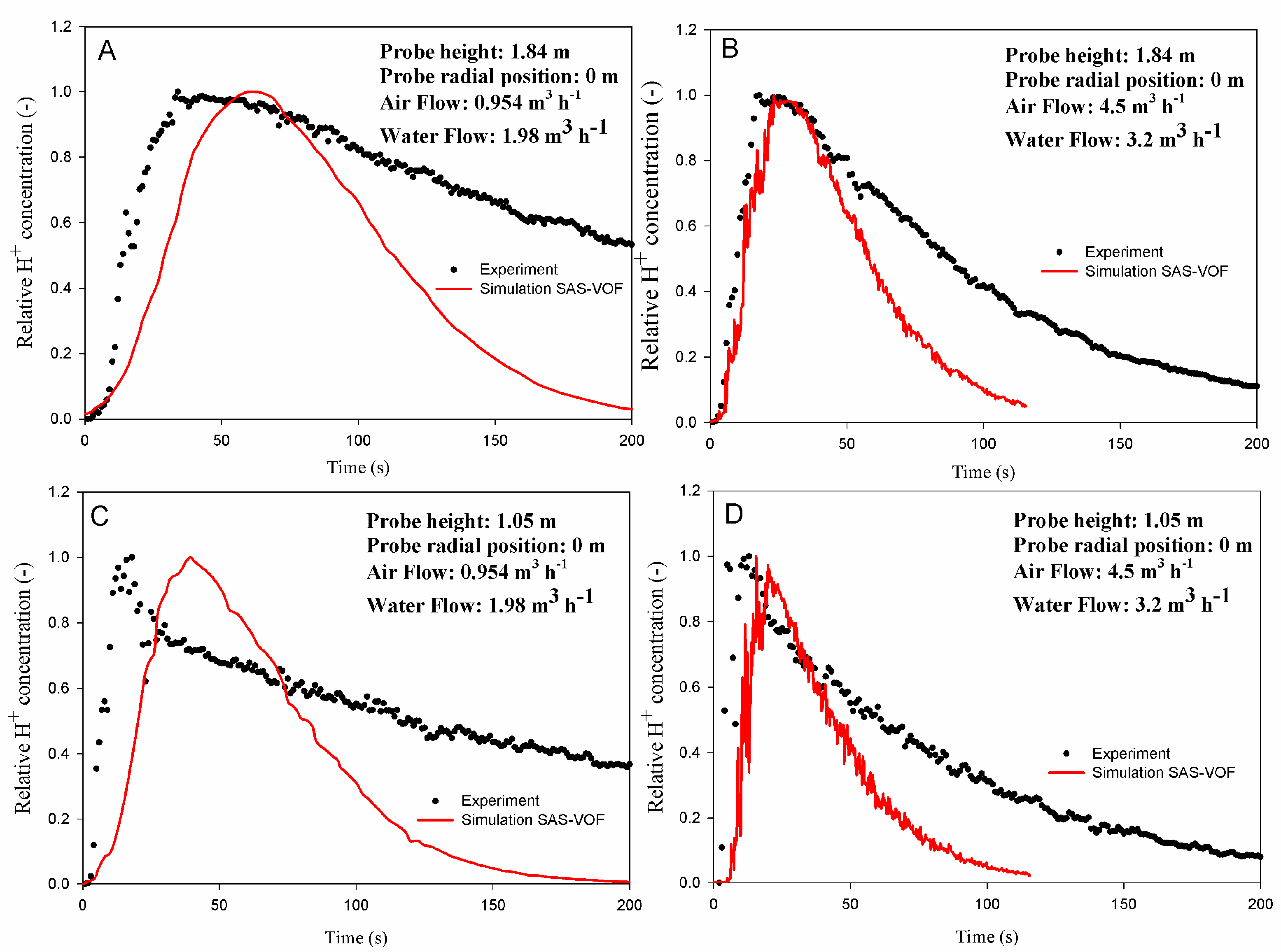
The temporal profiles of the tracer response for the simulations and experiments are shown in Figure 5. The profiles correspond to the centerline of the column at two axial locations (z = 1.05 and 1.84 m) for the two extreme flow scenarios. For the low-flow experiments (Figure 5A,C), the simulated response rose less quickly than the experimental response, and the simulated response peak was sharper than the experimental peak. After the rise, the experimental tracer concentration decreased at a much lower rate compared to simulations. Similar results were observed for the high-flow condition (Figure 5B,D). In this case, the rising part of the experimental tracer response was correctly simulated, but the simulated tracer concentration declined faster than the experimental data. Therefore, the simulation could not capture the level of back-mixing or the presence of fluid dead zones. Differences between pH data obtained from probes located at 1.05 and 1.84 m suggest that the tracer dispersed in an increasingly larger water volume along its path. Under high-flow conditions, the difference between the measured and simulated responses was smaller compared to the difference under low-flow conditions. The patterns shown in Figure 5 are consistent with other observations in batch bubble columns [36]. In prior studies, the LES-based models were shown to better capture the anisotropic bubble plume movement in a batch bubble column compared to some of the other models [36]. Compared to low gas flow rates, simulations better matched the experimental data for higher superficial gas velocities (>9 × 10⁻⁴ m s−1) [36]. In the present study, the superficial air velocities were much higher (≥6 × 10⁻³ m s−1).
In Figure 5, the difference between the experimental and simulated tracer data was probably a result of the presence of bubbles in the system that were not adequately accounted for by the selected combination of models. Compared to single-phase water flow, the presence of air in the two-phase system significantly increased the dispersion of the tracer. Bubbles increased the residence time of the tracer in the column, and thus mixing was improved. Gas flow rate is known to have a stronger influence on liquid phase dispersion in a bubble column compared to the flow rate of the liquid [37]. Although the simulations in Figure 5 did not exactly reproduce experimental tracer responses, the reduced local perturbations in both the simulated and experimental concentration profiles were noticeable in Figure 5 compared to the case for the single-phase flow shown in Figure 4. Perhaps, although the mesh size is adequate for resolving turbulence and velocity fields, it may not be adequate for resolving air bubbles with the precision that the VOF model needs. It might not be, therefore, suitable to choose the VOF model to simulate the system of this work on a workstation because the scale of the fluid domain is too large for implementing the significantly finer mesh required. Consequently, the combination of SAS-VOF models can only be used in ANSYS Fluent® for small, two-phase systems.
In order to quantitatively compare the experimental and simulated data, mean residence times (trm) and their variances (σt2, σθ2) were calculated based on the different measurement locations. The results are summarized in Table 4. The mean residence times confirmed the qualitative observations in Figure 4 and Figure 5: the actual experimental residence time of the tracer was substantially and consistently longer than the simulations. The experimental variance values confirmed a high level of axial mixing, suggesting that for the low-flow settings, the system approached a perfectly mixed state (Table 4). For all combinations of air and water flow rates, the simulations suggested a system that approximated plug flow.
Irrespective of the axial and radial locations of the measurement points, the values of the mixing parameters were essentially identical for any given combination of the air and water flow conditions (Table 4). This confirmed good radial dispersion. In the axial direction, the lower part of the column (z = 1.05 m) located close to the entrance points of the air and water phases had higher values of the liquid phase dispersion (greater variances σθ2) compared to the zone higher up (z = 1.84 m) (Table 4).
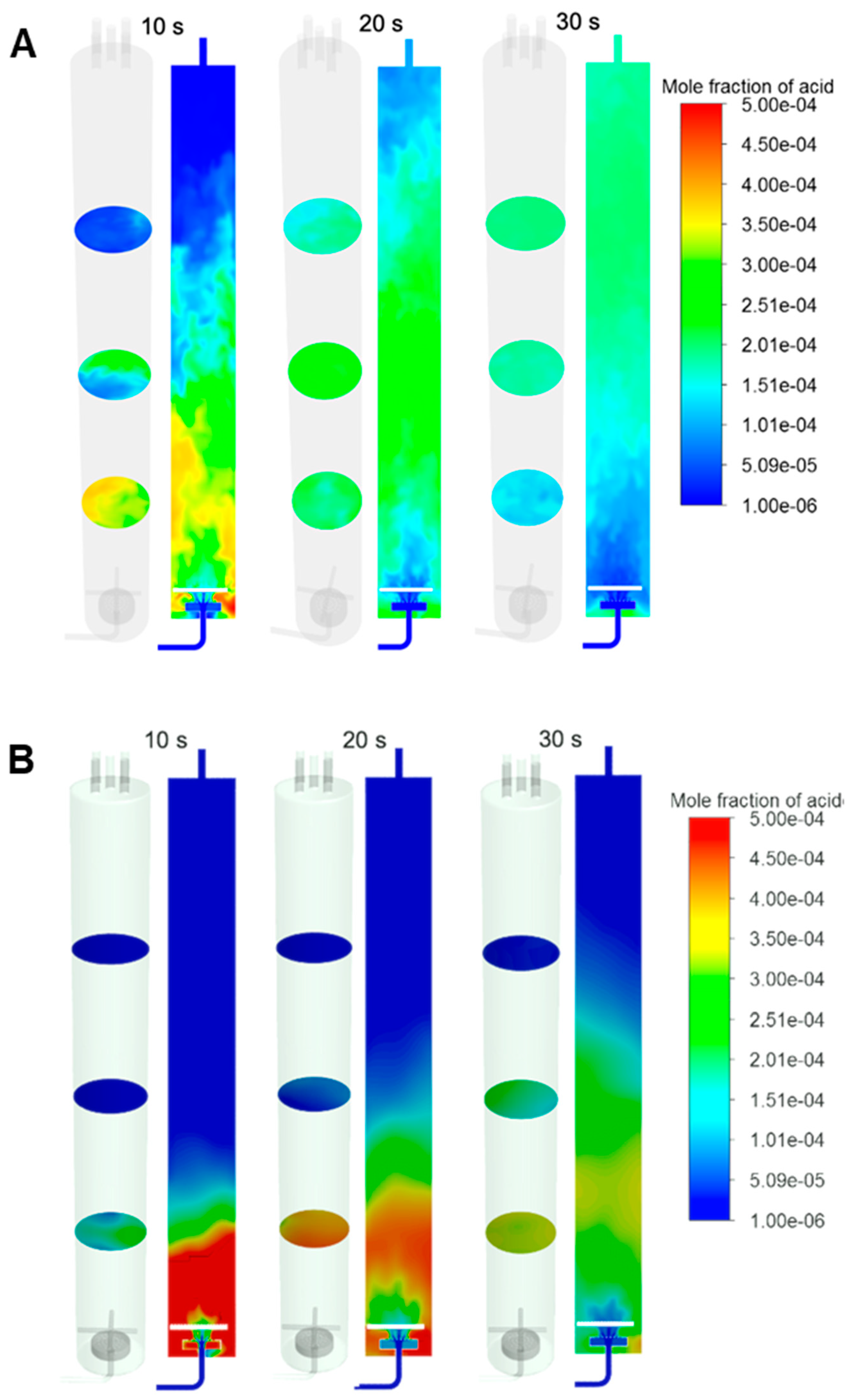
The temporal evolution of the contours of the tracer mole fraction is shown in Figure 6, 10, 20, and 30 s after tracer injection. Contours for longer elapsed times are included in Figures S5 and S6 (Supplementary Materials). The vertical sections shown represent planes at the center of the column, parallel to the flow (Figure 6). The circular horizontal sections shown represent planes at three different heights across the direction of the flow. For the high flow rates of the two phases (Figure 6A), axial dispersion was evident in the bottom third of the column and in the central plane (elapsed time = 10 s). In the upper sections, the tracer was almost completely dispersed axially. Contours for elapsed times of 20 and 30 s showed no differences in the axial direction. For low-flow combinations (Figure 6B), the tracer was not axially dispersed by the elapsed times of 10 or 20 s after injection. For an elapsed time of 30 s, the horizontal circular plane halfway up the column showed a pattern comparable to that of the corresponding high-flow condition (Figure 6A). This was logical, as the variances for the relevant relative residence times were of a similar order (Table 4). As more air bubbles were introduced into the water, they created turbulence in the surrounding fluid due to the drag forces and vortices generated by their motion. This causes turbulence that ultimately affects the dynamics of the system by increasing radial and axial mixing.
In summary, in the present work, the SAS model was appropriate for simulating tracer dispersion in single-phase water flows. For two-phase flows, the VOF model, which was the only two-phase model available in ANSYS Fluent® along with the SAS model, proved unable to simulate the effects of bubbles on tracer mixing. The grid size of the meshes that were optimum for resolving velocity and turbulence fields was not fine enough to accurately resolve the gas-liquid interphase. Similar conclusions were reported by Islam et al. for their study on single bubble rising behaviors [38]. As the concentration of bubbles increases, the interfacial area increases, and the mesh requirement increases exponentially [39].
If the mesh is too coarse, the VOF model predictions are imprecise and, therefore, seem to limit the prediction of the gas-liquid interactions and the macroscopic flow patterns [20,26,40]. Two-phase flows continue to be inadequately modeled by the commonly used fluid dynamic models because limitations in computational power necessitate the use of submodels that rely on a large number of empirical parameters [20,41]. An accurate accounting of the local interphase properties in bubble columns is necessary, especially for cases with a high gas holdup. A promising E-L approach combining VOF and a level-set (LS) method has accurately predicted the interphase topology of a bubble rising in a quiescent liquid [28], but its utility for modeling complex flow in a significantly sized bubble column with a high gas holdup remains to be proven.

4. Conclusions

To our best knowledge, this is the first work assessing the abilities of CFD to describe tracer dispersion in a continuous flow column at industrial scale. LES-based models outperformed RANS. Moreover, LES models were qualitatively and quantitatively satisfactory for predicting the dispersion of tracer in a single-phase (water-only) continuous flow bubble column under all conditions. For two-phase air-water systems, these models could be used only in conjunction with VOF-type models in ANSYS Fluent®, limiting their applicability. For the biphasic system, the turbulence models qualitatively predicted the time evolution of the tracer concentration but lacked a quantitative prediction capacity. The biphasic VOF model appeared to have limited applicability if a fine mesh refinement was impractical.

Supplementary Materials

The following supporting information can be downloaded at: https://www.mdpi.com/article/10.3390/app13169250/s1, Figure S1. Comparison of meshes: Simulated radial profiles of relative velocity (relative to maximum velocity) at different heights in the column with single phase flow (water only) (realizable k-ε; Qw = 1.98 m3 h−1). The number of elements in meshes 1, 2, 3, 4, and 5 were 325430, 394114, 613250, 694189, and 789452, respectively. Figure S2. Comparison meshes for air-water flow: Radial profiles of relative water velocity (relative to the maximum velocity) at different column heights (Qw = 1.98 m3 h−1; Qa = 0.954 m3 h−1). The number of elements in meshes 2, 3, 4, 5 were 394114, 613250, 694189, and 789452, respectively. Figure S3. Comparison of meshes for air-water flow: Radial profiles of relative air velocity (relative to the maximum velocity) at different column heights (Qw = 1.98 m3 h−1; Qa = 0.954 m3 h−1). The number of elements in meshes 2, 3, 4, 5 were 394114, 613250, 694189, and 789452, respectively. Figure S4. Values of l0/Δ calculated for air-water simulations (SAS-VOF model) 40 s after tracer injection: (A) Qw = 1.98 m3 h−1, Qa = 0.954 m3 h−1; (B) Qw = 3.2 m3 h−1, Qa = 4.5 m3 h−1. Figure S5. Contours of acid concentration (mole fraction) in air-water continuous flow bubble column (Qw = 3.2 m3 h−1; Qa = 4.5 m3 h−1) obtained by Fluent simulations. Elapsed times after tracer injection are shown at the bottoms of the columns. (A) At the center of the column, parallel to flow; (B) At different heights (horizontal planes, normal to flow). Figure S6. Contours of acid concentration (mole fraction) in air-water continuous flow bubble column (Qw = 1.98 m3 h−1; Qa = 0.954 m3 h−1) obtained by Fluent simulations. Elapsed times after tracer injection are shown at the bottoms of the columns. (A) At the center of the column, parallel to flow; (B) At different heights (horizontal planes, normal to flow). Table S1. Details of the meshes evaluated.

Author Contributions

Conceptualization, J.J.G.-R. and A.S.-M.; methodology, L.L.-R. and A.S.-M.; investigation, J.V.-A., E.L.-H. and L.L.-R.; writing-original draft, J.J.G.-R.; writing—review and editing, F.B., Y.C., A.S.-M. and F.G.-C. funding acquisition, J.J.G.-R., A.S.-M. and F.G.-C.; project administration, J.J.G.-R., A.S.-M. and F.G.-C. All authors have read and agreed to the published version of the manuscript.

Funding

This work was funded by the State Research Agency (grant PID2019-109476RB-C22) of the Spanish Ministry of Science, Innovation, and Universities; the Operative Program FEDER Andalucía 2014–2020 Framework (grant UAL2020-BIO-A2078); and the University of Almería (grant PPUENTE2020/013).

Institutional Review Board Statement

Not applicable.

Informed Consent Statement

Not applicable.

Data Availability Statement

Data is available from the corresponding author on request.

Conflicts of Interest

The authors declare that they have no known competing financial interests or personal relationships that could have appeared to influence the work reported in this paper.

Nomenclature

CFDComputational fluid dynamics
DESDetached eddy simulation
DNSDirect numerical simulation
EARSMExplicit algebraic Reynolds stress model
E-EEuler-Euler schemes
E-LEuler-Lagrange approaches
kTurbulent kinetic energy (J kg−1)
LESLarge eddy simulation
lLength scale (m)
l0Length scale defined by Equation (1) (m)
MSDModeled stress depletion
maMass flow rate (kg s−1)
QaVolume flow rate (m3 h−1)
RANSReynolds-averaged Navier-Stokes models
ReReynolds number
RNGRenormalization group
RSMReynolds stress model
rRadial position of sensor from central axis (m)
SASScale-adaptive simulation
SSTShear stress transport
SST-SASShear stress transport scale-adaptive simulation
tiDuration of tracer pulse (s)
trmResidence time (s)
uaSuperficial velocity (m s−1)
VLVolume of water in the bubble column (m3)
VOFVolume-of-fluid model
xiMole fraction of H+ in tracer (-)
zAxial location of a pH sensor above the column base (m)
ΔSize of the cell (m)
εRate of dissipation of turbulent kinetic energy (J kg−1 s−1)
μViscosity (Pa s)
ρDensity (kg m−3)
σt2Variance of the residence time (s2)
σθ2Variance of the relative residence time (-)
ωSpecific energy dissipation rate (J kg−1 s−1)

References

  1. Chisti, Y. Mass Transfer. In Kirk-Othmer Encyclopedia of Chemical Technology; John Wiley & Sons, Inc.: Hoboken, NJ, USA, 2017; pp. 1–70. [Google Scholar]
  2. Deckwer, W.D. Bubble Column Reactors; Wiley: Chichester, UK, 1992. [Google Scholar]
  3. Shah, Y.T.; Kelkar, B.G.; Godbole, S.P.; Deckwer, W.-D. Design Parameters Estimations for Bubble Column Reactors. AIChE J. 1982, 28, 353–379. [Google Scholar] [CrossRef]
  4. Ho, D.; Kim, K.; Earmme, T.; Kim, C. Enhancing Gas–Liquid Volumetric Mass Transfer Coefficient. J. Ind. Eng. Chem. 2020, 87, 1–17. [Google Scholar] [CrossRef]
  5. Kantarci, N.; Borak, F.; Ulgen, K.O. Bubble Column Reactors. Process Biochem. 2005, 40, 2263–2283. [Google Scholar] [CrossRef]
  6. Chen, P.; Duduković, M.P.; Sanyal, J. Three-Dimensional Simulation of Bubble Column Flows with Bubble Coalescence and Breakup. AIChE J. 2005, 51, 696–712. [Google Scholar] [CrossRef]
  7. Ebadi Amooghin, A.; Jafari, S.; Sanaeepur, H.; Kargari, A. Computational Fluid Dynamics Simulation of Bubble Coalescence and Breakup in an Internal Airlift Reactor: Analysis of Effects of a Draft Tube on Hydrodynamics and Mass Transfer. Appl. Math. Model. 2015, 39, 1616–1642. [Google Scholar] [CrossRef]
  8. Zahradnik, J.; Fialova, M.; Ruzicka, M.; Drahos, J.; Kastanek, F.; Thomas, N.H. Duality of the Gas-Liquid Flow Regimes in Bubble-Column Reactors. Chem. Eng. Sci. 1997, 52, 3811–3826. [Google Scholar] [CrossRef]
  9. Shu, S.; Vidal, D.; Bertrand, F.; Chaouki, J. Multiscale Multiphase Phenomena in Bubble Column Reactors: A Review. Renew. Energy 2019, 141, 613–631. [Google Scholar] [CrossRef]
  10. Behkish, A.; Lemoine, R.; Sehabiague, L.; Oukaci, R.; Morsi, B.I. Gas Holdup and Bubble Size Behavior in a Large-Scale Slurry Bubble Column Reactor Operating with an Organic Liquid under Elevated Pressures and Temperatures. Chem. Eng. J. 2007, 128, 69–84. [Google Scholar] [CrossRef]
  11. Krishna, R.; Sie, S.T. Design and Scale-up of the Fischer–Tropsch Bubble Column Slurry Reactor. Fuel Process. Technol. 2000, 64, 73–105. [Google Scholar] [CrossRef]
  12. López-Rosales, L.; Sánchez-Mirón, A.; García-Camacho, F.; Place, A.R.; Chisti, Y.; Molina-Grima, E. Pilot-Scale Outdoor Photobioreactor Culture of the Marine Dinoflagellate Karlodinium Veneficum: Production of a Karlotoxins-Rich Extract. Bioresour. Technol. 2018, 253, 94–104. [Google Scholar] [CrossRef] [Green Version]
  13. Chisti, Y. Shear Sensitivity. In Encyclopedia of Industrial Biotechnology; John Wiley & Sons, Inc.: New York, NY, USA, 2009; pp. 1–40. [Google Scholar]
  14. Kim, J.Y.; Kim, B.; Nho, N.-S.; Go, K.-S.; Kim, W.; Bae, J.W.; Jeong, S.W.; Epstein, N.; Lee, D.H. Gas Holdup and Hydrodynamic Flow Regime Transition in Bubble Columns. J. Ind. Eng. Chem. 2017, 56, 450–462. [Google Scholar] [CrossRef]
  15. Camacho Rubio, F.; Sánchez Mirón, A.; Cerón García, M.C.; García Camacho, F.; Molina Grima,, E.; Chisti, Y. Mixing in Bubble Columns: A New Approach for Characterizing Dispersion Coefficients. Chem. Eng. Sci. 2004, 59, 4369–4376. [Google Scholar] [CrossRef]
  16. Kawase, Y.; Moo-Young, M. Mixing Time in Bioreactors. J. Chem. Technol. Biotechnol. 1989, 44, 63–75. [Google Scholar] [CrossRef]
  17. Levenspiel, O.; Lai, B.W.; Chatlynne, C.Y. Tracer Curves and the Residence Time Distribution. Chem. Eng. Sci. 1970, 25, 1611–1613. [Google Scholar] [CrossRef]
  18. Liu, Y.; Hinrichsen, O. Study on CFD–PBM Turbulence Closures Based on k–ε and Reynolds Stress Models for Heterogeneous Bubble Column Flows. Comput. Fluids 2014, 105, 91–100. [Google Scholar] [CrossRef]
  19. Khan, Z.; Bhusare, V.H.; Joshi, J.B. Comparison of Turbulence Models for Bubble Column Reactors. Chem. Eng. Sci. 2017, 164, 34–52. [Google Scholar] [CrossRef]
  20. Dhotre, M.T.; Deen, N.G.; Niceno, B.; Khan, Z.; Joshi, J.B. Large Eddy Simulation for Dispersed Bubbly Flows: A Review. Int. J. Chem. Eng. 2013, 2013, 343276. [Google Scholar] [CrossRef]
  21. Huang, Q.; Yang, C.; Yu, G.; Mao, Z.S. CFD Simulation of Hydrodynamics and Mass Transfer in an Internal Airlift Loop Reactor Using a Steady Two-Fluid Model. Chem. Eng. Sci. 2010, 65, 5527–5536. [Google Scholar] [CrossRef]
  22. Masood, R.M.A.; Rauh, C.; Delgado, A. CFD Simulation of Bubble Column Flows: An Explicit Algebraic Reynolds Stress Model Approach. Int. J. Multiph. Flow 2014, 66, 11–25. [Google Scholar] [CrossRef]
  23. López-Rosales, L.; Sánchez-Mirón, A.; Contreras-Gómez, A.; García-Camacho, F.; Battaglia, F.; Zhao, L.; Molina-Grima, E. Characterization of Bubble Column Photobioreactors for Shear-Sensitive Microalgae Culture. Bioresour. Technol. 2019, 275, 1–9. [Google Scholar] [CrossRef]
  24. Deen, N.G.; Solberg, T.; Hjertager, B.H. Large Eddy Simulation of the Gas–Liquid Flow in a Square Cross-Sectioned Bubble Column. Chem. Eng. Sci. 2001, 56, 6341–6349. [Google Scholar] [CrossRef]
  25. Laborde-Boutet, C.; Larachi, F.; Dromard, N.; Delsart, O.; Schweich, D. CFD Simulation of Bubble Column Flows: Investigations on Turbulence Models in RANS Approach. Chem. Eng. Sci. 2009, 64, 4399–4413. [Google Scholar] [CrossRef]
  26. Tabib, M.V.; Roy, S.A.; Joshi, J.B. CFD Simulation of Bubble Column—An Analysis of Interphase Forces and Turbulence Models. Chem. Eng. J. 2008, 139, 589–614. [Google Scholar] [CrossRef]
  27. Ekambara, K.; Dhotre, M.T. CFD Simulation of Bubble Column. Nucl. Eng. Des. 2010, 240, 963–969. [Google Scholar] [CrossRef]
  28. Ansari, M.R.; Azadi, R.; Salimi, E. Capturing of Interface Topological Changes in Two-Phase Gas–Liquid Flows Using a Coupled Volume-of-Fluid and Level-Set Method (VOSET). Comput. Fluids 2016, 125, 82–100. [Google Scholar] [CrossRef]
  29. McClure, D.D.; Norris, H.; Kavanagh, J.M.; Fletcher, D.F.; Barton, G.W. Validation of a Computationally Efficient Computational Fluid Dynamics (CFD) Model for Industrial Bubble Column Bioreactors. Ind. Eng. Chem. Res. 2014, 53, 14526–14543. [Google Scholar] [CrossRef]
  30. McClure, D.D.; Aboudha, N.; Kavanagh, J.M.; Fletcher, D.F.; Barton, G.W. Mixing in Bubble Column Reactors: Experimental Study and CFD Modeling. Chem. Eng. J. 2015, 264, 291–301. [Google Scholar] [CrossRef]
  31. Wei, C.N.; Ochiai, S. Tracer-Response Techniques in Evaluation of Mixing in Reactors. The Mixing Characteristics of an Industrial Liquid-Phase Reactor Are Evaluated from the Transient Response of the Tracer Concentration at the Outlet. Plant/Oper. Prog. 1983, 2, 123–126. [Google Scholar] [CrossRef]
  32. Sánchez Mirón, A.; Cerón García, M.C.; García Camacho, F.; Molina Grima, E.; Chisti, Y. Mixing in Bubble Column and Airlift Reactors. Chem. Eng. Res. Des. 2004, 82, 1367–1374. [Google Scholar] [CrossRef] [Green Version]
  33. Luo, H.-P.; Al-Dahhan, M.H. Verification and Validation of CFD Simulations for Local Flow Dynamics in a Draft Tube Airlift Bioreactor. Chem. Eng. Sci. 2011, 66, 907–923. [Google Scholar] [CrossRef]
  34. Wiora, J.; Wiora, A. Measurement Uncertainty Calculations for PH Value Obtained by an Ion-Selective Electrode. Sensors 2018, 18, 1915. [Google Scholar] [CrossRef] [PubMed] [Green Version]
  35. Ashton, N. Recalibrating Delayed Detached-Eddy Simulation to Eliminate Modelled-Stress Depletion. In Proceedings of the 23th AIAA Computational Fluid Dynamics Conference, Denver, CO, USA, 5–9 June 2017; AIAA AVIATION Forum; American Institute of Aeronautics and Astronautics: Reston, VA, USA, 2017. [Google Scholar]
  36. Sanchez-Forero, D.I.; Silva, J.L., Jr.; Silva, M.K.; Bastos, J.C.S.C.; Mori, M. Experimental and Numerical Investigation of Gas-Liquid Flow in a Rectangular Bubble Column with Centralized Aeration Flow Pattern. Chem. Eng. Trans. 2013, 32, 1561–1566. [Google Scholar] [CrossRef]
  37. Han, S.; Zhou, J.; Jin, Y.; Loh, K.C.; Wang, Z. Liquid Dispersion in Gas-Liquid-Solid Circulating Fluidized Beds. Chem. Eng. J. 1998, 70, 9–14. [Google Scholar] [CrossRef]
  38. Islam, M.T.; Ganesan, P.B.; Cheng, J.; Uddin, M.S. Single Bubble Rising Behaviors in Newtonian and Non-Newtonian Fluids with Validation of Empirical Correlations: A Computational Fluid Dynamics Study. Eng. Rep. 2020, 2, e12100. [Google Scholar] [CrossRef] [Green Version]
  39. Akhtar, M.A.; Tadé, M.; Pareek, V. Simulations of Bubble Column Reactors Using a Volume of Fluid Approach: Effect of Air Distributor. Can. J. Chem. Eng. 2007, 85, 290–301. [Google Scholar] [CrossRef]
  40. Xiao, F.; Dianat, M.; McGuirk, J.J. LES of Turbulent Liquid Jet Primary Breakup in Turbulent Coaxial Air Flow. Int. J. Multiph. Flow 2014, 60, 103–118. [Google Scholar] [CrossRef] [Green Version]
  41. Zhang, Z.; Chen, Q. Prediction of Particle Deposition onto Indoor Surfaces by CFD with a Modified Lagrangian Method. Atmos. Environ. 2009, 43, 319–328. [Google Scholar] [CrossRef] [Green Version]
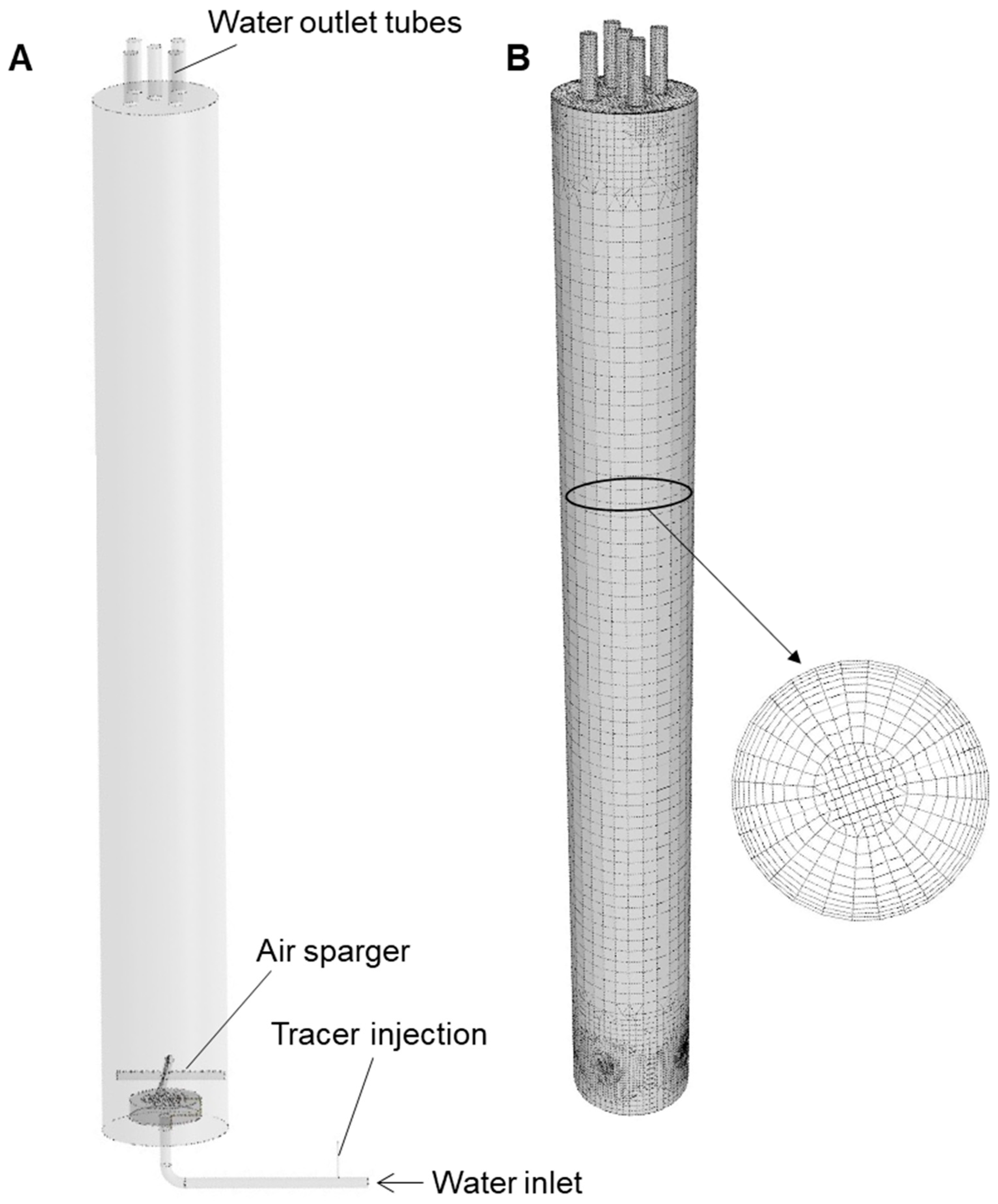
Figure 1. Geometric details of the bubble column, the air sparger, the liquid distributor, and the tracer injection port (A). Depiction of the optimum mesh (mesh of 6.9 × 10⁵ elements) (B).
Applsci 13 09250 g001
Figure 2. Radial profile of relative velocity (relative to the maximum velocity) of water at different column heights during single-phase flow (water only) as simulated with the realizable k-ε turbulence model (Qw = 1.98 m3 h−1; mesh of 3.9 × 10⁵ elements).
Applsci 13 09250 g002
Figure 3. Radial profile of relative velocity (relative to the maximum velocity) at different heights in the column simulated for water-air flow (Qw = 1.98 m3 h−1, Qa = 0.954 m3 h−1) using the realizable k-ε/dispersed Eulerian biphasic model. (A) velocities for the water phase; (B) velocities for air phase. Mesh of 3.9 × 10⁵ elements.
Applsci 13 09250 g003
Figure 4. Comparison of the relative acid concentration (tracer) versus time in single-phase water flow (Qw = 3.2 m3 h−1) for the turbulence models evaluated and the experimental results. (A,B) tracer concentrations at 1.84 m above the column base at centerline for RANs and LES models, respectively. Mesh of 3.9 × 10⁵ elements; (C,D) tracer concentrations at 1.05 m above the column base at centerline for RANs and LES models, respectively. Mesh of 6.9 × 10⁵ elements.
Applsci 13 09250 g004
Figure 5. Comparison of the relative acid concentration versus time in two-phase continuous flow bubble column. Measured and simulated data are compared. Simulations used the SAS-VOF two-phase model. (A) Centerline tracer concentration at z = 1.84 m (Qw = 1.98 m3 h−1, Qa = 0.954 m3 h−1); (B) centerline tracer concentration at z = 1.84 m (Qw = 3.2 m3 h−1, Qa = 4.5 m3 h−1); (C) centerline tracer concentration at z = 0.105 m (Qw = 1.98 m3 h−1, Qa = 0.954 m3 h−1); (D) centerline tracer concentration at z = 1.05 m (Qw = 3.2 m3 h−1, Qa = 4.5 m3 h−1). Mesh of 6.9 × 10⁵ elements.
Applsci 13 09250 g005
Figure 6. Contours of tracer concentration (mole fraction of H+) for two-phase continuous flow bubble column, obtained using Fluent simulations. The time after tracer injection is shown beside each column. (A) Qw = 3.2 m3 h−1, Qa = 4.5 m3 h−1; (B) Qw = 1.98 m3 h−1, Qa = 0.954 m3 h−1.
Applsci 13 09250 g006
Table 1. CFD solver settings used in ANSYS simulations.
ParameterSetting
Pressure-velocity couplingSIMPLE
Spatial discretizationLeast squares cell based
PressureStandard
Momentum2nd Order upwind
Turbulent kinetic energy2nd Order upwind
Turbulent dissipation rate2nd Order upwind
Specific dissipation rate2nd Order upwind
Intermittency2nd Order upwind
Momentum thickness Re1st Order upwind
Tracer concentration2nd Order upwind
Transient state formulation1st Order implicit
Table 2. Physical properties of fluids.
FluidWaterTracer
(HCl, 37% w/w)
Air
Molar mass
(kg kmol−1)
18.15236.46028.996
Density, ρ
(kg m−3)
998.21190.0122.5 × 10−2
Viscosity, μ
(Pa s)
10.03 × 10−42.0 × 10−5178.94 × 10−7
Surface tension
(N m−1)
72.75 × 10⁻³--
Table 3. Flow settings.
FlowLowHigh
ti
(s)
2.52.5
xi0.22460.2246
Qw
(m3 h−1)
1.983.2
uw
(m s−1)
0.01280.0207
mw
(kg s−1)
0.5490.887
Qa
(m3 h−1)
0.9544.5
ua
(m s−1)
0.06120.0291
Qa/VL
(vvm)
0.1850.872
ma
(kg s−1)
32.46 × 10−5153.13 × 10−5
Table 4. Comparison of measured and simulated tracer residence times (trm) and variance.
Flow Settingsz (m)r (m)ExperimentsSimulations (SAS + VOF)
trm (s)σt2 (s2)σθ2 (-)trm (s)σt2 (s2)σθ2 (-)
Qw = 1.98 m3 h−1;
Qa = 0.954 m3 h−1
1.050221.836,8430.7559.212100.35
1.050.1218.135,5300.7560.712090.33
1.840227.934,6790.6782.916030.23
1.840.1244.437,8900.6380.616000.25
Qw = 3.2 m3 h−1;
Qa = 4.5 m3 h−1
1.05077.044090.7434.85140.43
1.050.176.141930.7235.85230.41
1.84083.540780.5944.65400.28
1.840.190.744440.5444.05380.28
Disclaimer/Publisher’s Note: The statements, opinions and data contained in all publications are solely those of the individual author(s) and contributor(s) and not of MDPI and/or the editor(s). MDPI and/or the editor(s) disclaim responsibility for any injury to people or property resulting from any ideas, methods, instructions or products referred to in the content.