M²GF: Multi-Scale and Multi-Directional Gabor Filters for Image Edge Detection

Abstract

An image edge detection algorithm using multi-directional and multi-scale Gabor filters is proposed in this paper. The main merit of this method is that high edge detection accuracy can be obtained while maintaining noise robustness. The approach proposed in this paper consists of three procedures: firstly, the transformation to the CIE L*a*b* color space, which has a wide shading area and uniform distribution; secondly, under different scales, the edge feature information of the image is extracted from several different directions by Gabor filters, and a new edge strength map is obtained by feature fusion; thirdly, the new fused edge strength map is enhanced with local features, and a noise-resistant image edge detector is obtained under a novel hysteresis threshold calculation. The experiments illustrate that, compared to the methods involved, the designed edge detector outperforms by about 2% to 4%, and also shows competitive performance regarding the ability to handle noise.

1. Introduction

Edge detection [1] is a foundational task in image processing and computer vision. Edges refer to positions where the information of pixels change suddenly in gray or color images [2,3,4,5,6,7]. The information of edges is used in many image processing and analysis techniques, such as image segmentation [8,9,10], image retrieval [11,12,13], corner detection [14,15,16,17,18], etc. The edge detection results of images usually play a key role in certain applications [19,20]. In addition, humans perceive color images more abundantly than colorless images [21,22]. In conclusion, for color images, an efficient and convenient edge detection algorithm is indispensable for many downstream tasks of computer vision.

In the past 40 years, there has been some progress in the research of edge detection approaches, which can be roughly divided into three branches [23]: fusion-based methods, gradient-based methods and vector-based methods. The former obtains the final edge result by fusing individual detected edge of channel components [24]. The core idea of the multi-dimensional gradient-based method aims to calculate the direction and intensity of each edge pixel [25]. The way that the vector properties of image pixels are not changed in the whole process of detection is described as vector-based methods;the edge algorithm based on the color morphological gradient [26], for example, avoids the processing of pixel value fusion. This paper mainly explores the multi-dimensional gradient-based method.

The main idea of the multi-dimensional gradient method is to find the direction and intensity of the edge and fuse them effectively before the hysteresis threshold. In 1977, Navatia, one of the first researchers to study edge detectors for color images, proposed a method that presents image data through brightness and two chrominance channels, and obtains edge maps in each individual component independently using Huckel edge detectors [22]. Robinson [27] also proposed a method for color edge detection in the same year. The 24 directional derivatives were computed and the one with the largest magnitude was chosen as the gradient. A color edge detection algorithm [28] was designed by Tsang that can suppress pseudo-edge pixels, which are the most important and common problem in edge detection. In order to solve the problem of the missing direction of edge pixels, Scharcanski and Venetsanopoulos [29] proposed a method of edge detection using local direction operators. It is precisely because the directional information of edge pixels is essential and relevant in various image analysis tasks [30,31,32,33,34]. Furthermore, a color edge detection method based on edge rendering, which combines gradient and intelligent routing, was proposed [35].

The Canny edge detector [36], as a milestone, has been in development for nearly four decades, and many improved algorithms have been proposed on this basis. Kanade believed that the magnitude and direction of the edge extracted by the Canny detector is the key to obtain high-quality edge detection [37], so it was introduced into color edge detection. It has been illustrated that Gabor filters resemble the perception of the human visual system [38,39,40]. Liu and Wechsler pointed out the merits of Gabor filters in extracting local features of images [41]. Zhang used a set of multi-scale and multi-directional Gabor filters to smooth edges and detect corners using the amplitude response and angle response [16]. In this paper, the CIE L*a*b space is adopted because it is sensitive to human visual perception. Then, the edge intensity map is obtained by smoothing the image with multi-scale and multi-direction Gabor filters. The Gabor filters with smaller scale are sensitive to noise but have high edge resolution and edge localization ability. In contrast, Gabor filters with large scale have better noise robustness, but poor accuracy. The edge features of the obtained multiple channels are fused to be processed in local feature enhancement, hysteresis threshold and edge refinement for edge detection. It is compared with Color Canny, Laplacian, CMG, improved Sobel, AGDD, ColorED and so on [20,42,43]. The accuracies of edge detectors are evaluated on the input images of BSD500 and NYUD datasets. And through the FOM measure, the noise robustness of the algorithms are evaluated. It can be seen from the experimental results that the proposed detector has good quality of edge detection.

The main contributions of our proposed method are as follows:

• A set of Gabor filters is used to attain rich and detailed features of edge under different scales and channels.
• A novel fusion strategy is proposed to obtain more accurate features of edge that are not disturbed by noise.
• A new method for calculating hysteresis threshold is designed to obtain the edge detection results with high accuracy and robust noise.

The organizational structure of this article is shown below. The conversion of the color space is introduced in Section 2 firstly. Then, the multi-directional and multi-scale Gabor filters are also introduced. In Section 3, the designed edge detector is presented. The schematic diagrams and the fused edge strength maps (ESMs) of the Gabor filters are given. In Section 4, a novel color edge detection scheme is designed, which has higher accuracy and better noise robustness. A comprehensive evaluation of the performance of the proposed mechanism is presented in Section 5. Finally, the analysis and conclusion as well as the prospect are given.

2. Related Work

In this section, the conversion of color space is introduced first. Then, the multi-directional Gabor filters with multi-scale are presented.

2.1. The Conversion of RGB Space to CIE L*a*b* Space

The CIE L*a*b* color space was published by the International Commission on Illumination in 1976. The CIE L*a*b* space can better reflect the color difference of objects. Therefore, it has demonstrated an unparalleled representation of visual information and is widely used in various visual tasks [44,45]. The RGB color space cannot be directly converted to CIE L*a*b* color space. The CIE XYZ [46] color space is required as a medium. The conversion of the RGB to the CIE XYZ is

$$\left[\begin{array}{c}X\\ Y\\ Z\end{array}\right]=\left[\begin{array}{ccc}0.4124& 0.3575& 0.1804\\ 0.2128& 0.7152& 0.0722\\ 0.0193& 0.1192& 0.9502\end{array}\right]\left[\begin{array}{c}R\\ G\\ B\end{array}\right].$$

(1)

The conversion of the CIE XYZ to the CIE L*a*b* is

$$L^{*}=116f(Y/Y_0)-16,$$

$$a^{*}=500[f(X/X_0)-f(Y/Y_0)],$$

$$b^{*}=200[f(Y/Y_0)-f(Z/Z_0)],$$

(2)

$$f\left(t\right)=\left\{\begin{array}{cc}{t}^{1/3},\hfill & \mathrm{if} t>0.008856\hfill \\ 7.787t+4/29,\hfill & \mathrm{otherwise}\hfill \end{array}\right.,$$

(3)

where $X_0=95.047$, $Y_0=100$ and $Z_0=108.883$, which are the CIE standard illuminator with three color values.

In Figure 1, the original images, the corresponding gray-scale images and the images of L*, a* and b* channels are shown in the first to the fifth rows, respectively. In the picture of “petal” in the first column on the left, the area of petals and stems marked by the red circle is not easy to be distinguished in the gray-scale image. But it is easy in the corresponding image in the a* and b* channel because of the difference in chromaticity. As the region marked by the red circle in the gray-scale picture of “Pottery figurine” shows, the difference between the plant and the back wall in the corresponding gray-scale image is small, which causes it to be covered by the background. However, its overall shape and structure are revealed in the b* channel of the image. The lines of branches are discontinuous and fuzzy in the gray-scale picture of “Puppy”, while these lines are completed and the outline is clear in b* channel of the image. The red flower is overlapped with the background in the region marked by the circle in the picture of “Cat”. The lines and outlines in the a* channel of the image are depicted more accurately than in the gray-scale image, owing to chroma. Therefore, using the CIE L*a*b* color space is very beneficial for extracting detailed information of the edges.

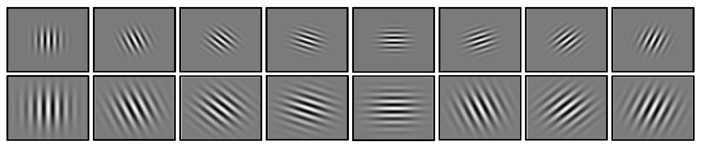
2.2. The Multi-Scale and Multi-Directional Gabor Filter

The Gabor filter, as a linear filter, is alike to the consciousness of the human visual because of the specific representations. Therefore, it is applied to the edge detection of the image. The response of the Gabor filter can be viewed as the product of sine/cosine wave Gaussian functions. The total, real and imaginary components of the Gabor filter are presented as

$$\begin{array}{c}\hfill g(x,y;f,\theta )=\frac{f^2}{\pi \gamma \eta }exp\left(-\left(\frac{f^2}{{\gamma }^2}{x}^{\prime 2}+\frac{f^2}{{\eta }^2}{y}^{\prime 2}\right)\right)\left(cos\left(2\pi f{x}^{\prime }\right)+jsin\left(2\pi f{x}^{\prime }\right)\right),\end{array}$$

$$x^{\prime }=xcos\theta +ysin\theta ,$$

$$y^{\prime }=-xsin\theta +ycos\theta ,$$

(4)

where x and y refer to the spatial coordinates into an image I, and $\gamma$ and $\eta$ are constants, which represent the sharpness along the horizontal and vertical axis, respectively. The central frequency of the filter is f. And $\theta$ is the rotation angle. It can be observed from Equation (4) that the scale is related to central frequency f. A low center frequency indicates a large-scale Gabor filter, which has a good noise robustness, while a high center frequency indicates a small-scale Gabor filter, which has better localization of the edges in the image. The real and imaginary components of the Gabor filter is shown in Figure 2a,b, respectively.

The first column in the Figure 3, from left to right, is a ladder edge, an angular edge, a Y-shaped edge, an X-shaped edge and a star edge. And the second and third columns of the Figure 3 depict the absolute values of amplitude responses for different types of edge and Gabor filters in polar and Cartesian coordinates, respectively. The Gabor filter is anisotropic, which can effectively extract the information of edge. And the relatively different responses can be observed in the area $T_i$ with different gray values. The multi-scale and multi-directional Gabor filter is extremely powerful for edge detection.

Considering the more convenient expression of the multi-scale filter, the scale factor $\sigma$ is added in the Gabor filter, and $f_{\sigma }$ represents the central frequency of scale $\sigma$. For an input discrete image $I\left(\mathbf{z}\right)$, $\mathbf{z}$ = ${(u,v)}^T$, in addition, the filter along different orientations needs to be used to extract local variation information around pixels. A set of discretized multi-scale Gabor filters can be obtained by taking different center frequencies f:

$$\begin{array}{c}\begin{array}{cc}\hfill \phi (u,v;f,\sigma ,k)=& \frac{f_{\sigma }^2}{\pi \gamma \eta }exp\left(-\left(\frac{f_{\sigma }^2}{{\gamma }^2}{u}^{\prime 2}+\frac{f_{\sigma }^2}{{\eta }^2}{v}^{\prime 2}\right)\right)\hfill \\ & ·exp\left(j2\pi f_{\sigma }{u}^{\prime }\right)\hfill \end{array}\\ u^{\prime }=ucos{\theta }_k+vsin{\theta }_k,\\ v^{\prime }=-usin{\theta }_k+vcos{\theta }_k,\\ {\theta }_k=\frac{\pi k}{K},k=0,1,\dots ,K-1\end{array}$$

(5)

where the number of K is directions, and ${\theta }_k$ is the k-th orientation. The amplitude response of the discrete Gabor filters along the orientation ${\theta }_k$ at the scale $f_{\sigma }$ is calculated by the convolution operator,

$$\begin{array}{cc}\hfill \psi (u,v;f,\sigma ,k)& =I\otimes \phi (u,v;f,\sigma ,k)\hfill \\ \hfill & =\sum _{u_p}\sum _{v_q}I(u-u_p,v-v_q)\phi (u,v;f,\sigma ,k),\hfill \end{array}$$

(6)

where “⊗” denotes the convolution.

The Gabor filters with eight orientations at two scales are shown in Figure 4. As a result, a set of the Gabor filters along the different orientations at the different scales can reflect the intensity variation around the edge pixels completely.

3. The Proposed Edge Detection

In this section, using the multi-directional Gabor filter with multi-scale, the ESMs of the three channels (L*, a* and b*) are presented. Furthermore, the fused edge features are calculated. Finally, a novel edge detection algorithm is derived by processing the fused features.

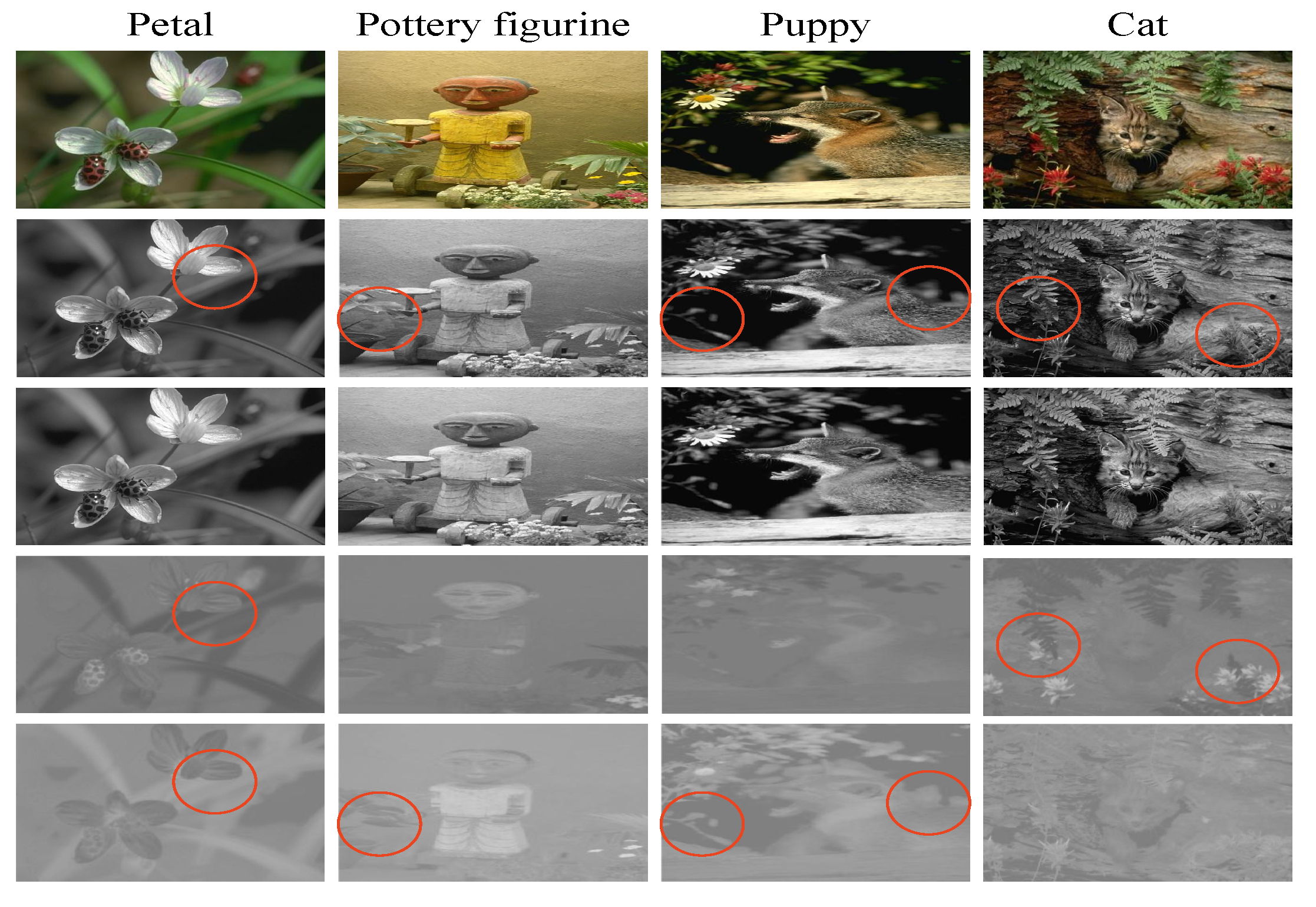
3.1. The ESMs of the Color Image and the Proposal of Fused Edge Features

Canny [36] pointed out that the optimal filter should have three criteria: (i) Good detection. (ii) Good localization. (iii) Only one response to a single edge. Smoothing the edges with a large-scale Gaussian kernel will cause the edge to blur and lose a lot of detail. This situation is especially obvious in the texture area, while the small-scale Gaussian kernel is very sensitive to noise. Under this situation, the scales and the orientations should be considered for the optimal filters design, which is regarded as a indispensable step in edge detection.

From the aforementioned analysis, the multi-directional Gabor filters with multi-scale has better noise robustness and higher edge accuracy. The max operator in Equation (8) refers to selecting the ”optimal” smoothing kernel [47] for each pixel from the Gabor filters. The ESMs from the multi-directional and multi-scale Gabor filters of an image are defined by

$$\zeta \left(\mathbf{z}\right)=\underset{k=0,1,2,\dots ,K-1}{max}\left\{|I\otimes \psi (u,v;f,\sigma ,k\left)\right|\right\},$$

(7)

When a color image is converted to the L*a*b* space, the use of Equation (7) smooths the L*, a* and b* channels, respectively. Then, according to the ESMs of the three channels, an overlay operation is adopted, which can achieve better filtering effects. In the end, the fused ESM can be calculated.

The fused feature map according to Equation (8) is able to resolve the influence of the blurring effect caused by chromaticity while maintaining high accuracy, and noise robustness. To a certain extent, the proposed approach can be summarized as seeking the fusion of edge feature maps by the multi-scale and multi-direction Gabor filter.

$$\xi \left(\mathbf{z}\right)=\sqrt[n]{{\zeta }_1\left(\mathbf{z}\right)·{\zeta }_2\left(\mathbf{z}\right)\dots ·{\zeta }_n\left(\mathbf{z}\right)},$$

(8)

where n represents the number of selected center frequencies.

The following Figure 5 depicts an example diagram of the fusion of edge feature maps.

Comparing the ESM1, ESM2 and the fused ESM in Figure 6, the original image is depicted in Figure 6a, which adds noise with Gaussian standard deviation ${\epsilon }_w=15$ before being smoothed by multi-direction Gabor filters of multi-scale. The ESM1 with a low central frequency $f_1$ ($f_1$ = 0.2) is illustrated in Figure 6b. As can be observed in Figure 6b, its large scale allows for more edge stretching on the ESM2 but is rarely polluted by noise. As the central frequency increases to $f_2$ ($f_2$ = 2), as can be seen in Figure 6c, the impact of noise on ESM is intensified, while the edge stretching effect of ESM1 is reduced, and more details of pixels are obtained. The reason is that large-scale ESM2 has strong robustness to noise. As depicted in Figure 6d, the fused ESM inherits the advantages of ESM1 and ESM2 at two different scales, with the small edge stretching effect and noise robustness.

3.2. Proposed Edge Detection

The outline of the proposed algorithm is as follows:

(i)

Convert color images to L*a*b* space.

(ii)

Extract edge strength maps from the each channel by multi-directional Gabor filters with multi-scale, and the fused edge feature is attained by the computation of ESMs in terms of Equation (8).

(iii)

Calculate the global and local average changes of the image, ${\overline{s}}_{Global}\left(\mathbf{z}\right)$ and ${\overline{s}}_{Local}\left(\mathbf{z}\right)$:

$${\overline{s}}_{Global}\left(\mathbf{z}\right)=\frac{1}{M·N}\sum _{\mathbf{z}}\xi \left(\mathbf{z}\right),$$

(9)

$${\overline{s}}_{Local}\left(\mathbf{z}\right)=\frac{1}{W^2}\sum _{\tau \in Q}\xi (\mathbf{z}+\tau )),$$

(10)

where $M·N$ refers to the dimension of the image, $\xi \left(\mathbf{z}\right)$ is the fusion of features in Equation (8). The Q is a matrix with side length W, whose values are all ones. And the Q is convolved with $\mathbf{z}$ while $\tau$ is the stride. The visual system is simulated to perform contrast equalization on the improved fusion of ESM, which is defined as

$$\tilde{\xi }\left(\mathbf{z}\right)=\frac{\xi \left(\mathbf{z}\right)}{\overline{s}+0.5{\overline{s}}_{Local}\left(\mathbf{z}\right)}.$$

(11)

(iv)

Apply the non-maxima suppression for each pixel, the gradient modulus $\tilde{\xi }\left(\mathbf{z}\right)$ and orientation $\theta \left(k\right)$ are used to determine whether it is the maximum of $\tilde{\xi }\left(\mathbf{z}\right)$.

(v)

Set the upper and lower limitations, which are determined by the histogram of the fused edge feature of the input image. The dimension of the image is $M·N$, and the coefficients ${\beta }_{low}$ and ${\beta }_{up}$$\in [0,1]$:

$$T_{up}=\tilde{\xi }\left({\mathbf{z}}_{[{\beta }_{up}·M·N]}\right),$$

(12)

$$T_{low}=\tilde{\xi }\left({\mathbf{z}}_{[{\beta }_{low}·M·N]}\right),$$

(13)

where the symbol “[]” is down-integer operation, ${\mathbf{z}}_{[{\beta }_{up}·M·N]}$ and ${\mathbf{z}}_{[{\beta }_{low}·M·N]}$ represent the $[{\beta }_{up}·M·N]$th pixel and the $[{\beta }_{low}·M·N]$th pixel listed the ESM from smallest to largest.

(vi)

Make the hysteresis decision. The determination of edge pixels is implemented in two stages. All the pixels whose value of the fused ESM exceeds $T_{up}$ are recognized as edge pixels. A candidate edge pixel with values of fused feature between $T_{up}$ and $T_{low}$ is regarded as an edge pixel if it can be connected with strong edge pixels in the four- or eight-neighborhood criterion.

A flow diagram of the proposed approach is depicted in Figure 7.

4. Experiments

In this section, the complete property results of the proposed algorithm are presented and compared with six kinds of detectors, such as [20,31,35]. The precision–recall curve is used to assess the results on the BSDS500 [48] and NYUD [49] datasets. The capabilities of six competitive methods are compared by means of detection accuracy and noise robustness.

4.1. The Superiority of CIE L*a*b* Color Space

Comparing with the RGB color space, the CIE L*a*b* color space has more obvious edges information in Figure 8. The results are illustrated in Figure 8e–g that the relatively complete edge detection results can be attained by the R, G, and B channels of the images. However, the detected results fail to show large differences, which leads to the loss of some edge details. As the L*, a*, and b* channels of the images and their corresponding detected results in Figure 8h–m show, although the detected result of the image in the a* channel is not ideal and the missing portion is more serious, large differences can be observed in L* and b* channels. And the overlay operation is used later. Obviously, in the region marked by two red circles in “Puppy”, the result of the edge detection is relatively continuous and complete. Not only are different brightness levels displayed but there are also large differences in chromaticity.

The distributions of pixel values of “Puppy” image in RGB and CIE L*a*b* models are depicted in Figure 9a,b. The values of features in the L*, a* and b* channels are normally higher than those in the R, G and B, channels. And there is a huge difference in the pixel values in each channel. In addition, the mean value of pixels in each channel can indicate the color gamut merit of L*a*b*. And the larger difference in the pixel values is very useful to extract edge information, which also explains the necessity of using the L*a*b* color space.

4.2. PR Curve Assessment

The PR curve [50,51,52] is a recognized performance indicator for evaluating the results of edge detection with corresponding ground truths (GTs). The rates of precision and recall are calculated by

$$Y_{precision}=\frac{n_{TP}}{n_{TP}+n_{FP}},$$

(14)

$$Y_{recall}=\frac{n_{MT}}{n_{MT}+n_{UM}},$$

(15)

where $n_{TP}$, $n_{FP}$, $n_{MT}$, and $n_{UM}$ are true and false positive detection pixels, and matched and unmatched ground truth pixels, respectively. The distance between any point on the PR curve and the origin, and the area enclosed by the PR curve (average precision (AP) [53]) are the indexes by which to evaluate the quality of the detection results. And the performance of detection is judged by R50 under a high recall rate [51]. The F-measure is calculated by accuracy and recall:

$$F=\frac{2·Y_{precision}·Y_{recall}}{Y_{precision}+Y_{recall}}.$$

(16)

4.3. FOM Index Assessment

The noise robustness of the edge detection results is tested by Pratt’s figure of merit (FOM) [54]. The pseudo-pixels and positioning errors are considered in the calculation. The number of edge pixels in the ground truth and the detected map are represented by $n_g$ and $n_e$, respectively. Then, FOM is calculated as follows:

$$FOM=\frac{1}{max(n_g,n_e)}\sum _{j=1}^{n_e}\frac{1}{1+\frac{d^2\left(j\right)}{4}},$$

(17)

where d(j) represents the distance from the from the j-th detected pixel to the corresponding label pixel. A value of 1 indicates a perfect result.

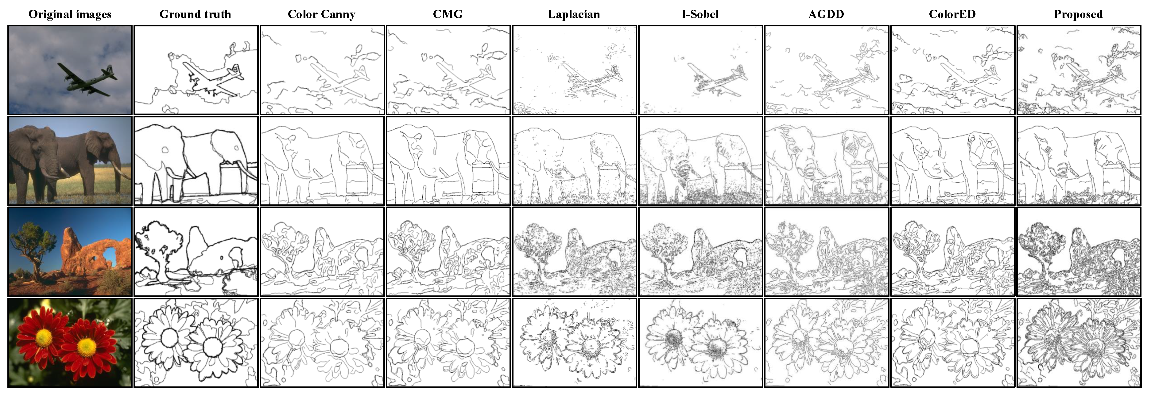
4.4. Experiments on the BSDS and NYUD Dataset

The BSDS and NYUD dataset are widely used for the performance comparison of edge detection methods. Many works have been evaluated on it recently.

On the BSDS datasets, the proposed method achieves the maximum area in the PR curves of the compared approaches, which are depicted in Figure 10a. The results of six edge detection algorithms on the NYUD dataset are depicted in Figure 10b. Although the algorithm proposed in this paper is not as good as some methods ([42,43]) based on deep learning in performance, these methods need an extra training process and more parameter operations. In addition, the algorithm designed is higher than most algorithms in the index of F-measure and AP. It is because the designed approach uses the L*a*b* color space, Gabor filters and some local detail processing, which can accurately obtain the information of edges. In addition, the application of multi-scale and multi-direction technology makes it have better anti-noise performance. At the same time, the indexes of $F_{ODS}$, $F_{OIS}$, and $R50$ are illustrated in

Table 1. Evaluation indicators obtained on the BSDS dataset.

Methods	${\mathit{F}}_{\mathbf{ODS}}$	${\mathit{F}}_{\mathbf{OIS}}$	AP	R50
Color Canny [37]	0.563	0.576	0.570	0.578
Laplacian [30]	0.598	0.615	0.583	0.725
I-Sobel [31]	0.581	0.587	0.586	0.693
CMG [26]	0.611	0.636	0.607	0.751
ColorED [35]	0.617	0.629	0.618	0.771
AGDD [20]	0.634	0.651	0.632	0.797
Proposed	0.672	0.695	0.652	0.828

and

Table 2. Evaluation indicators obtained on the NYUD dataset.

Methods	${\mathit{F}}_{\mathbf{ODS}}$	${\mathit{F}}_{\mathbf{OIS}}$	AP	R50
CMG [26]	0.651	0.661	0.637	0.773
ColorED [35]	0.673	0.667	0.653	0.794
AGDD [20]	0.677	0.716	0.629	0.804
HED [42]	0.741	0.757	0.749	0.900
RCF [43]	0.765	0.780	0.760	0.888
Proposed	0.685	0.708	0.689	0.843

, and the designed approach achieves better performance.

In this experiment, four original color images are depicted in the first column of Figure 11. The ground truths of the corresponding images are presented in the second column of Figure 11. The detection results of the Color Canny method [37], the CMG method [26], the Laplacian method [30], the I-Sobel method [31], the AGDD method [20], the ColorED method [35] and the proposed method are depicted in the 3th, 4th, 5th, 6th, 7th, 8th and 9th columns of Figure 11, respectively. Intuitively, the designed method can accurately extract and detect edge information.

In addition, when noise of ${\epsilon }_w=15$ is added to the above four images, the performance of the different approaches is as depicted in Figure 12. The noisy color images are depicted in the first column of Figure 12. The ground truth maps of the noisy images are depicted in the second column of Figure 12. The detection results of the Color Canny method [37], the CMG method [26], the Laplacian method [30], the I-Sobel method [31], the AGDD method [20], the ColorED method [35] and the proposed method are shown in the 3th, 4th, 5th, 6th, 7th, 8th and 9th columns of Figure 12, respectively. The FOMs of the different edge detection methods are described in

Table 3. Comparison of FOMs.

Methods	Plane	Elephant	Tree	Flower
Color Canny [37]	0.6675	0.6726	0.7731	0.7886
CMG [26]	0.7223	0.7434	0.7745	0.7678
Laplacian method [30]	0.6127	0.6439	0.6328	0.6456
I-Sobel method [31]	0.6517	0.6219	0.6473	0.6756
ColorED [35]	0.7713	0.7616	0.7925	0.8053
AGDD [20]	0.7753	0.7727	0.8006	0.8124
Proposed	0.7837	0.7842	0.8075	0.8168

. The comparison illustrates that the designed approach has better noise robustness. However, it is complicated and time-consuming to use multi-direction Gabor filter banks with multiple scales. And the related running time test of the algorithms is presented in

Table 4. Running time test of algorithms (s).

Methods	Plane	Elephant	Tree	Flower
Color Canny [37]	2.252	2.732	2.029	2.067
CMG [26]	2.297	2.721	2.112	2.189
Laplacian method [30]	2.437	2.588	2.187	2.186
I-Sobel method [31]	2.271	2.734	2.125	2.154
ColorED [35]	6.810	7.078	6.936	6.859
AGDD [20]	5.287	5.968	5.853	5.684
Proposed	6.219	6.446	6.329	6.283

, in which the proposed algorithm takes a long time, but the strategy of sacrificing some time to obtain higher accuracy and more robust detection results is adopted.

5. Conclusions and Future Works

This paper presents an edge detector with high precision and strong anti-noise ability. The multi-directional Gabor filters with multi-scale were used to attain rich edge features. The novel fusion strategy was designed to attain more accurate edge features that are not disturbed by noise. The method for calculating the hysteresis threshold was designed to obtain the edge detection results with high accuracy and robust noise. Experimental results illustrate that the design has dominant performance, which is compared with some competitive edge detectors. Image edge detection is a fundamental work in the fields of computer vision. However, in the face of the actual visual task that integrates various unfavorable factors, the existing edge detection technology does not show a strong effect. We expect that on the basis of this research, not only can more researchers pay attention to edge detection but also some practical problems can be found and solved, which can inspire future research activities.

References

1. Jing, J.; Liu, S.; Wang, G.; Zhang, W.; Sun, C. Recent advances on image edge detection: A comprehensive review. Neurocomputing 2022, 503, 259–271. [Google Scholar] [CrossRef]
2. Torre, V.; Poggio, T.A. On Edge Detection. IEEE Trans. Pattern Anal. Mach. Intell. 1986, 8, 147–163. [Google Scholar] [CrossRef] [PubMed]
3. Upla, K.P.; Joshi, M.V.; Gajjar, P.P. An Edge Preserving Multiresolution Fusion: Use of Contourlet Transform and MRF Prior. IEEE Trans. Geosci. Remote Sens. 2015, 53, 3210–3220. [Google Scholar] [CrossRef]
4. Shui, P.; Zhang, W. Noise-robust edge detector combining isotropic and anisotropic Gaussian kernels. Pattern Recognit. 2012, 45, 806–820. [Google Scholar] [CrossRef]
5. Zhang, W.; Zhao, Y.; Breckon, T.P.; Chen, L. Noise robust image edge detection based upon the automatic anisotropic Gaussian kernels. Pattern Recognit. 2017, 63, 193–205. [Google Scholar] [CrossRef]
6. Li, Y.; Bi, Y.; Zhang, W.; Sun, C. Multi-Scale Anisotropic Gaussian Kernels for Image Edge Detection. IEEE Access 2020, 8, 1803–1812. [Google Scholar] [CrossRef]
7. Jing, J.; Liu, S.; Liu, C.; Gao, T.; Zhang, W.; Sun, C. A novel decision mechanism for image edge detection. In Proceedings of the International Conference on Intelligent Computing, Melbourne, Australia, 25–27 June 2021; Springer: Cham, Switzerland, 2021; pp. 274–287. [Google Scholar]
8. Shi, J.; Malik, J. Normalized cuts and image segmentation. IEEE Trans. Pattern Anal. Mach. Intell. 2000, 22, 888–905. [Google Scholar]
9. Comaniciu, D.; Meer, P. Mean shift: A robust approach toward feature space analysis. IEEE Trans. Pattern Anal. Mach. Intell. 2002, 24, 603–619. [Google Scholar] [CrossRef]
10. Ramirez Rivera, A.; Murshed, M.; Kim, J.; Chae, O. Background modeling through statistical edge-segment distributions. IEEE Trans. Circuits Syst. Video Technol. 2013, 23, 1375–1387. [Google Scholar] [CrossRef]
11. Manjunath, B.; Ma, W. Texture features for browsing and retrieval of image data. IEEE Trans. Pattern Anal. Mach. Intell. 1996, 18, 837–842. [Google Scholar] [CrossRef]
12. Cheng, M.; Mitra, N.J.; Huang, X.; Torr, P.H.S.; Hu, S. Global contrast based salient region detection. IEEE Trans. Pattern Anal. Mach. Intell. 2015, 37, 569–582. [Google Scholar] [CrossRef] [PubMed]
13. Zhang, S.; Tian, Q.; Lu, K.; Huang, Q.; Gao, W. Edge-SIFT: Discriminative binary descriptor for scalable partial-duplicate mobile search. IEEE Trans. Image Process. 2013, 22, 2889–2902. [Google Scholar] [CrossRef] [PubMed]
14. Shui, P.; Zhang, W. Corner Detection and Classification Using Anisotropic Directional Derivative Representations. IEEE Trans. Image Process. 2013, 22, 3204–3218. [Google Scholar] [CrossRef] [PubMed]
15. Zhang, W.; Sun, C.; Breckon, T.; Alshammari, N. Discrete curvature representations for noise robust image corner detection. IEEE Trans. Image Process. 2019, 28, 4444–4459. [Google Scholar] [CrossRef]
16. Zhang, W.; Wang, F.; Zhu, L.; Zhou, Z. Corner detection using Gabor filters. Iet Image Process. 2014, 8, 639–646. [Google Scholar] [CrossRef]
17. Zhang, W.; Shui, P. Contour-based corner detection via angle difference of principal directions of anisotropic Gaussian directional derivatives. Pattern Recognit. 2015, 48, 2785–2797. [Google Scholar] [CrossRef]
18. Zhang, W.; Sun, C.; Gao, Y. Image intensity variation information for interest point detection. IEEE Trans. Pattern Anal. Mach. Intell. 2023, 45, 9883–9894. [Google Scholar] [CrossRef]
19. Gary, L. Object knowledge changes visual appearance: Semantic effects on color afterimages. Acta Psychol. 2015, 161, 117–130. [Google Scholar]
20. Wang, F.; Shui, P. Noise-robust color edge detector using gradient matrix and anisotropic Gaussian directional derivative matrix. Pattern Recognit. 2016, 52, 346–357. [Google Scholar] [CrossRef]
21. Belen, M.; Gordon, W.; Piotr, D.; Diego, G. Special Section on Advanced Displays: A survey on computational displays: Pushing the boundaries of optics, computation, and perception. Comput. Graph. 2013, 37, 1012–1038. [Google Scholar]
22. Nevatia, R. A Color Edge Detector and Its Use in Scene Segmentation. IEEE Trans. Syst. Man Cybern. 1977, 7, 820–826. [Google Scholar]
23. Ruzon, M.; Tomasi, C. Edge, junction, and corner detection using color distributions. IEEE Trans. Pattern Anal. Mach. Intell. 2001, 23, 1281–1295. [Google Scholar] [CrossRef]
24. Topal, C.; Akinlar, C. Edge Drawing: A combined real-time edge and segment detector. J. Vis. Commun. Image Represent. 2012, 23, 862–872. [Google Scholar] [CrossRef]
25. Khotanzad, A.; Chen, J.Y. Unsupervised segmentation of textured images by edge detection in multidimensional feature. IEEE Trans. Pattern Anal. Mach. Intell. 1989, 11, 414–421. [Google Scholar] [CrossRef]
26. Evans, A.; Liu, X. A morphological gradient approach to color edge detection. IEEE Trans. Image Process. 2006, 15, 1454–1463. [Google Scholar] [CrossRef] [PubMed]
27. Robinson, G.S. Color Edge Detection. Opt. Eng. 1977, 16, 479–484. [Google Scholar] [CrossRef]
28. Tsang, W.; Tsang, P. Suppression of False Edge Detection Due to Specular Reflection in Color Images. Pattern Recognit. Lett. 1997, 18, 165–171. [Google Scholar] [CrossRef]
29. Scharcanski, J.; Venetsanopoulos, A. Edge detection of color images using directional operators. IEEE Trans. Circuits Syst. Video Technol. 1997, 7, 397–401. [Google Scholar] [CrossRef]
30. Tai, S.; Shihming, Y. A fast method for image noise estimation using Laplacian operator and adaptive edge detection. In Proceedings of the 2008 3rd International Symposium on Communications, Control and Signal Processing, St Julians, Malta, 12–14 March 2008; pp. 1077–1081. [Google Scholar]
31. Deng, C.; Ma, W.; Yin, Y. An edge detection approach of image fusion based on improved Sobel operator. In Proceedings of the 2011 4th International Congress on Image and Signal Processing, Shanghai, China, 15–17 October 2011; Volume 3, pp. 1189–1193. [Google Scholar]
32. Jing, J.; Gao, T.; Zhang, W.; Gao, Y.; Sun, C. Image feature information extraction for interest point detection: A comprehensive review. arXiv 2021, arXiv:2106.07929. [Google Scholar] [CrossRef]
33. Zhang, W.; Sun, C. Corner detection using multi-directional structure tensor with multiple scales. Int. J. Comput. Vis. 2020, 128, 438–459. [Google Scholar] [CrossRef]
34. Zhang, W.; Sun, C. Corner detection using second-order generalized Gaussian directional derivative representations. IEEE Trans. Pattern Anal. Mach. Intell. 2021, 43, 1213–1224. [Google Scholar] [CrossRef] [PubMed]
35. Akinlar, C.; Topal, C. ColorED: Color edge and segment detection by Edge Drawing (ED). J. Vis. Commun. Image Represent. 2017, 44, 82–94. [Google Scholar] [CrossRef]
36. Canny, J. A Computational Approach to Edge Detection. IEEE Trans. Pattern Anal. Mach. Intell. 1986, 8, 679–698. [Google Scholar] [CrossRef] [PubMed]
37. Kanade, T. Image Understanding Research at CMU. In Proceedings of the Image Understanding Workshop, Los Angeles, CA, USA, 23–25 February 1987; Volume 2, pp. 32–40. [Google Scholar]
38. Daugman, J.G. Uncertainty relation for resolution in space, spatial frequency, and orientation optimized by two-dimensional visual cortical filters. J. Opt. Soc. Am. A-Opt. Image Sci. Vis. 1985, 2, 1160–1169. [Google Scholar] [CrossRef] [PubMed]
39. Hill, P.; Achim, A.; Al-Mualla, M.E.; Bull, D. Contrast Sensitivity of the Wavelet, Dual Tree Complex Wavelet, Curvelet, and Steerable Pyramid Transforms. IEEE Trans. Image Process. 2016, 25, 2739–2751. [Google Scholar] [CrossRef] [PubMed]
40. Ni, Z.; Zeng, H.; Ma, L.; Hou, J.; Chen, J.; Ma, K. A Gabor Feature-Based Quality Assessment Model for the Screen Content Images. IEEE Trans. Image Process. 2018, 27, 4516–4528. [Google Scholar] [CrossRef]
41. Liu, C.; Wechsler, H. Gabor feature based classification using the enhanced fisher linear discriminant model for face recognition. IEEE Trans. Image Process. 2002, 11, 467–476. [Google Scholar]
42. Xie, S.; Tu, Z. Holistically-Nested Edge Detection. In Proceedings of the 2015 IEEE International Conference on Computer Vision (ICCV), Santiago, Chile, 7–13 December 2015; pp. 1395–1403. [Google Scholar]
43. Liu, Y.; Cheng, M.; Hu, X.; Jiawang, B.; Zhang, L.; Bai, X.; Tang, J. Richer Convolutional Features for Edge Detection. IEEE Trans. Pattern Anal. Mach. Intell. 2019, 41, 1939–1946. [Google Scholar] [CrossRef]
44. Jing, J.; Liu, S.; Li, P.; Zhang, L. The fabric defect detection based on CIE L*a*b* color space using 2-D Gabor filter. J. Text. Inst. 2016, 107, 1305–1313. [Google Scholar] [CrossRef]
45. Lei, T.; Zhang, Y.; Wang, Y.; Liu, S.; Guo, Z. A conditionally invariant mathematical morphological framework for color images. Inf. Sci. 2017, 387, 34–52. [Google Scholar] [CrossRef]
46. Liang, J.; Zhou, J.; Bai, X.; Qian, Y. Salient object detection in hyperspectral imagery. In Proceedings of the International Conference on Image Processing, Melbourne, Australia, 15–18 September 2013; pp. 2393–2397. [Google Scholar]
47. Alvarez, L.; Lions, P.L.; Morel, J.M. Image selective smoothing and edge detection by nonlinear diffusion. II. Siam J. Numer. Anal. 1992, 29, 845–866. [Google Scholar] [CrossRef]
48. Arbeláez, P.; Maire, M.; Fowlkes, C.; Malik, J. Contour detection and hierarchical image segmentation. IEEE Trans. Pattern Anal. Mach. Intell. 2011, 33, 898–916. [Google Scholar] [CrossRef] [PubMed]
49. Silberman, N.; Hoiem, D.; Kohli, P.; Fergus, R. Computer Vision—ECCV 2012: 12th European Conference on Computer Vision, Florence, Italy, October 7–13 2012; Proceedings, Part V 12; Springer: Berlin/Heidelberg, Germany, 2012; pp. 746–760. [Google Scholar]
50. Coleman, S.A.; Scotney, B.W.; Suganthan, S. Edge detecting for range data using Laplacian operators. IEEE Trans. Image Process. 2010, 19, 2814–2824. [Google Scholar] [CrossRef]
51. Dollár, P.; Zitnick, C.L. Fast edge detection using structured forests. IEEE Trans. Pattern Anal. Mach. Intell. 2014, 37, 1558–1570. [Google Scholar]
52. Bae, Y.; Lee, W.H.; Choi, Y.; Jeon, Y.W.; Ra, J.B. Automatic road extraction from remote sensing images based on a normalized second derivative map. IEEE Geosci. Remote Sens. Lett. 2015, 12, 1858–1862. [Google Scholar]
53. Martin, D.; Fowlkes, C.; Malik, J. Learning to detect natural image boundaries using local brightness, color, and texture cues. IEEE Trans. Pattern Anal. Mach. Intell. 2004, 26, 530–549. [Google Scholar] [CrossRef]
54. Pratt, W.K. Digital Image Processing; John Wiley and Sons, Incorporated: Hoboken, NJ, USA, 1978. [Google Scholar]
Figure 1. Four original color images and the corresponding images in different channels. (From top to the bottom, the gray-scale images and the images in L*, a* and b* channels are shown in the first row to the fifth row, respectively.)
Applsci 13 09409 g001
Figure 2. Examples of real and imaginary components of Gabor filter with the γ = 1.3, η = 2.5, f = 0.3 and θ = 2 3 π . (a) A real component of Gabor filter. (b) An imaginary component of Gabor filter.
Applsci 13 09409 g002
Figure 3. Magnitude responses of different types of edges and Gabor filters. (a) A ladder edge. (d) An angular edge. (g) A Y-shaped edge. (j) A X-shaped edge. (m) A star-shaped edge. (b,e,h,k,n) in the middle columns represent the absolute values of amplitude responses for different types of edges and Gabor filters in polar coordinates, respectively. (c,f,i,l,o) in the right columns represent the part of the magnitude responses for different types of edges and Gabor filters in Cartesian coordinates.
Applsci 13 09409 g003
Figure 4. A set of Gabor filters with eight orientations (from left to right, the orientations are 0, π 8 , π 4 , 3 π 8 , π 2 , 5 π 8 , 3 π 4 , 7 π 8 ) in the first column to the eighth column, respectively. The central frequency of the first row is f 1 ( f 1 = 0.1), and the second row is f 2 ( f 2 = 0.2). γ = 1, η = 2.
Applsci 13 09409 g004
Figure 5. Flow diagram of the integrated ESM.
Applsci 13 09409 g005
Figure 6. Depiction of the ESMs of an image: (a) a noisy image; (b) ESM1 at low f 1 ( f 1 = 0.2); (c) ESM2 at high f 2 ( f 2 = 2); and (d) fused ESM.
Applsci 13 09409 g006
Figure 7. The flow diagram the proposed method.
Applsci 13 09409 g007
Figure 8. The “Puppy” images in R, G, B, L*, a* and b* channels and their corresponding detection results: (a) the “Puppy” image; (bd) depict the “Puppy” in R, G and B channels; (eg) illustrate the detected results of R, G and B channels of the “Puppy”, respectively; (hj) describe the “Puppy” in L*, a* and b* channels; (km) show the results of L*, a* and b* channels of the “Puppy”, respectively.
Applsci 13 09409 g008
Figure 9. The magnitudes of pixel values of the “Puppy” image in RGB and CIE L*a*b* models. (a) The “Puppy” image in CIE L*a*b* space. (b) The “Puppy” image in RGB space.
Applsci 13 09409 g009
Figure 10. The results on the BSDS [48] and NYUD [49] datasets. (a) Detection performance based on the BSDS dataset. (b) Detection performance based on the NYUD dataset.
Applsci 13 09409 g010
Figure 11. Detection results of seven methods on four test images.
Applsci 13 09409 g011
Figure 12. Detection results of seven methods on four noisy color images.
Applsci 13 09409 g012