A Novel Autonomous Landing Method for Flying–Walking Power Line Inspection Robots Based on Prior Structure Data

Abstract

Hybrid inspection robots have been attracting increasing interest in recent years, and are suitable for inspecting long-distance overhead power transmission lines (OPTLs), combining the advantages of flying robots (e.g., UAVs) and climbing robots (e.g., multiple-arm robots). Due to the complex work conditions (e.g., power line slopes, complex backgrounds, wind interference), landing on OPTL is one of the most difficult challenges faced by hybrid inspection robots. To address this problem, this study proposes a novel autonomous landing method for a developed flying–walking power line inspection robot (FPLIR) based on prior structure data. The proposed method includes three main steps: (1) A color image of the target power line is segmented using a real-time semantic segmentation network, fusing the depth image to estimate the position of the power line. (2) The safe landing area (SLA) is determined using prior structure data, applying the trajectory planning method with geometric constraints to generate the dynamic landing trajectory. (3) The landing trajectory is tracked using real-time model predictive control (MPC), controlling FPLIR to land on the OPTL. The feasibility of the proposed method was verified in the ROS Gazebo environment. The RMSE values of the position along three axes were $0.1205,0.0976$ and $0.0953$, respectively, while the RMSE values of the velocity along these axes were 0.0426, 0.0345 and 0.0781. Additionally, experiments in a real environment using FPLIR were performed to verify the validity of the proposed method. The experimental results showed that the errors of position and velocity for the FPLIR landing on the lines were $6.18\times {10}^{-2}\mathrm{m}$ and $2.16\times {10}^{-2}\mathrm{m}/\mathrm{s}$. The simulation results as well as the experimental findings both satisfy the practical requirements. The proposed method provides a foundation for the intelligent inspection of OPTL in the future.

1. Introduction

OPTL, as a key component of the state grid infrastructure, is a primary means for the long-distance transmission of electric power, contributing significantly to the economic development of a stable nation. Due to their passage through harsh environments (e.g., deserts, mountains, forests, and rivers), OPTLs are easily affected by material deterioration, electrical flashover, and constant mechanical tension [1,2,3]. To efficiently and reliably transmit high-voltage electric power, OPTLs need to be routinely inspected for early fault detection [4]. In the US, the average cost of a half-hour blackout for medium and large industrial customers is USD 15,707, while it is nearly USD 94,000 for an 8 h interruption. Additionally, the growing global population and the over-reliance on electricity supply have created great demand for more efficient transmission line inspection strategies [5,6].

The original inspection method for OPTLs was human inspection, which requires inspectors to climb along the power line to detect faults. This is laborious, inefficient, and dangerous for inspectors [7]; therefore, robots have become important tools for OPTL inspection over the past three decades [8]. Currently, many studies focus mainly on climbing robots (e.g., multi-arm robots) and flying robots (e.g., UAVs). Climbing robots are suitable for short-distance inspections with heavier payloads, providing detailed and reliable inspection data due to being closer to the power lines. Nevertheless, bypassing large obstacles and landing on overhead power lines present great difficulties. Flying robots are flexible, low cost, and capable of collecting high-quality images. However, they are limited in terms of flight endurance and cannot accurately inspect OPTLs from close distances [9,10,11].

Hybrid robots have been a focus of attention in recent decades, combining the advantages of climbing robots with those of flying robots. They are suitable for long-distance inspections with more flexibility. The flight mechanism can land on power lines and fly over obstacles, while the walking mechanism can walk along the OPTLs [12,13]. The existing landing methods of hybrid robots only allow the robots to approach power lines from the top [12,14,15,16] or the bottom [17,18,19]. However, these hybrid robots are unstable when walking on power lines due to their mechanical structure. In addition, power lines are flexible cable structures with slopes; when hybrid robots land on power lines, they may slip or lose control. As a result, autonomous landing methods for the developed FPLIR should be investigated to ensure safe landing on power lines. This challenge can be broken down into four main issues: (1) identify power lines in the observable space; (2) estimate the status of the robot using the onboard sensors; (3) plan a trajectory that satisfies the dynamic constraints of the robot; (4) track the trajectory under the work conditions [14]. To address these problems, this study proposes a novel landing method for the developed FPLIR based on prior structure data. The main contributions can be outlined as follows:

Firstly, a novel approach is proposed for determining an SLA before landing on the line. The SLA is calculated based on prior structure data derived from the complex working conditions of the OPTLs. In addition, the SLA is considered to be the basis for a safe landing.

Then, a trajectory planning method based on geometric constraints is applied. These constraints are defined by the landing characteristics, the structural features of the FPLIR, and prior structural data. By determining the desired position, the method generates a collision-free and dynamically feasible trajectory to guide the FPLIR to a zero-speed landing on the power line.

Finally, an MPC controller is designed considering the characteristics of the FPLIR. The MPC controller applies a feedback control strategy to the generated landing trajectory and optimizes the trajectory in real time. This approach enables the accurate tracking of the target landing trajectory even under complex conditions.

This paper is organized as follows: Section 2 summarizes the previous works. Section 3 introduces the hardware and software of the landing line system. Section 4 presents the details of the proposed method. Section 5 shows and analyzes the results of the simulations and real experiments. The discussion is presented in Section 6. Finally, the conclusions are drawn in Section 7.

2. Related Works

2.1. Power Line Detection

The existing image-based methods for power line detection can be divided into traditional and deep-learning-based methods, as listed in

Table 1. Summary of the literature related to power line detection.

Method Category	Author/Method	Advantages	Limitations
Traditional method	Yan et al. [20], Li et al. [21], Yang et al. [22], Cerón et al. [23], Song et al. [24]	Simple model, fast and automatic, low data requirements	Low noise resistance, low extraction accuracy
Deep learning-based method	Holistically Nested Edge Detection [25], DeepContour [26], DeepEdge [27] Zhang et al. [28], Madaan et al. [29]	Diverse use of information, high scene applicability, high extraction accuracy	Complex model, high data requirements, low extraction efficiency

. Traditional methods have focused on low-level local features, such as gradient, luminance, texture, and other prior information. Power lines are assumed to be straight lines or polynomial curves with the lowest intensity in the image and parallel to each other. Yan et al. [20] adopted Radon transform to extract line segments, and then connected the segments into the whole line using the grouping method and the Kalman filter. Li et al. [21] proposed a knowledge-based power line detection method using the Pulse Coupled Neural Network (PCNN) to remove background noise from the images. Yang et al. [22] proposed an adaptive thresholding approach, Hough transforms and the Fuzzy C-Means (FCM) clustering algorithm for power line detection, removing spurious lines using the properties of power lines. Cerón et al. [23] proposed a method called Circle-Based Search (CBS) for detecting power lines by searching for lines between two opposite points. Song et al. [24] proposed a sequential local-to-global power line detection method based on a graph-cut model. However, the limitations of these methods are still obvious when applied to a real environment. For instance, manually tuning dozens of parameters makes it difficult to achieve the optimal result for each image during the inspection. Thus, when the parameters are fixed, the methods tend to produce more false positives and negatives on a dataset.

Deep learning-based methods have a strong ability to learn multiscale features and perceive global information, and they can produce high-level representations of objects in natural images. State-of-the-art CNN-based edge detectors, such as Holistically Nested Edge Detection [25], DeepContour [26] and DeepEdge [27], can be applied to produce very-high-quality edge maps. Then, the edge maps can be used by traditional straight-line detection methods (e.g., Hough transform). Zhang et al. [28] developed an accurate power line detection method using convolutional and structured features, improving the detection accuracy. Madaan et al. [29] treated power line detection as a semantic segmentation task, adopting an expansive convolutional network to develop a power line detection framework. Semantic segmentation using CNN is a highly accurate method. CNNs are robust to change in illumination and scenarios, reducing the chances of false positives and negatives. However, it is well known that CNN, and particularly segmentation networks (e.g., SegNet [30] or DeepLab [31]), usually have a high computational cost. This fact is crucial for FPLIR due to payload limitations and the need for real-time detection. The STDC-Seg [32,33,34] is used to address this problem, as it is able to provide real-time semantic segmentation with low-computing cost and high accuracy.

2.2. Robot Landing Method

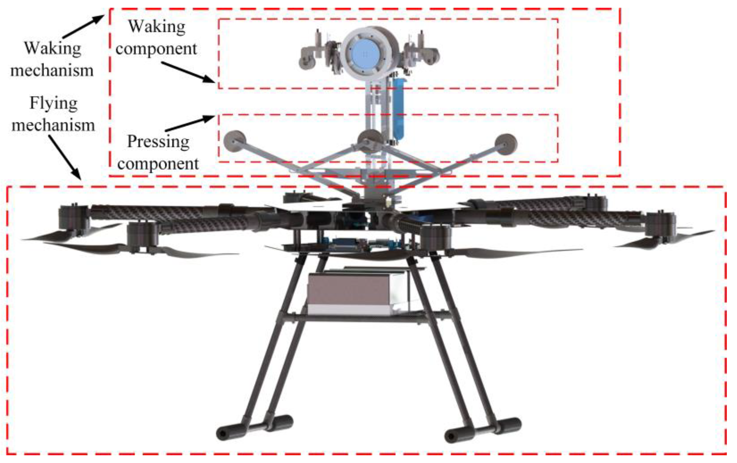
With regard to methods of landing on a wall, Erginer et al. [35] proposed a method combining a PD attitude controller and vision-based tracking to allow UAVs to land autonomously on a stationary platform. Mellinger et al. [36] defined a planned trajectory as a series of segments, each of which was executed by a linear controller for the landing trajectory. Thomas et al. [37] developed a method for planning trajectories considering actuator and sensor constraints, enabling a quadrotor with a gripper to land on inclined surfaces. Mao et al. [38] proposed a vision-based wall landing method that used a combination of Apriltags and Visual Inertial Odometry (VIO) to land on the wall without using a motion capture system. The typical method for landing on walls is by colliding at terminal velocities, which is not safe for the landing of an FPLIR on a power line.

With regard to methods of landing on a power line or cylinder, Popek et al. [39] presented an autonomous perching concept for UAVs, integrating vision-based perception, path planning and motion control on an aerial robot with limited processing capability. They realized the landing of a UAV with a manipulator on a cylinder. This required the establishment of constraints with respect to the drones and the cylinders, but was difficult for power lines. Mirallès et al. [14] used a cascaded P/PI controller to align the UAV with the power line and to assist the pilot in controlling the UAV landing on the power line from above. It was semi-automatic. Ramon-Soria et al. [15] used position-based visual servoing (PBVS) to land a UAV with soft jaws on a pipe. Hang et al. [16] proposed a heterogeneous landing platform that allowed multi-rotor robots to land on common structures, such as streetlights and the edges of buildings. The terminal speed on landing was not taken into account. Thomas et al. [17] proposed image-based visual servoing (IBVS), enabling a UAV to land on a cylindrical structure from below, which is difficult to construct geometric models of FPLIR and power lines.

To ensure safe landing, the FPLIR reaches the desired final pose with zero velocity. Based on the above work, in this study, trajectory planning is modeled as a nonlinear constrained optimization problem, using lines and segments to design a new cost function and constraints.

With regard to trajectory tracking methods, Ahmed et al. [40] proposed an extended backstepping nonlinear controller, which permitted multi-rotor UAVs to land on a moving platform. Wang et al. [41] used a hybrid of the $H_2/H_{\infty }$ technique to ensure that UAVs could track the desired trajectory under the influence of uncertainties and disturbances. Escareño et al. [42] used a hierarchical control strategy that was based on a combination of sliding mode and adaptive strategies. Meanwhile, they considered adaptive trajectory tracking in the presence of parameter uncertainties and constant wind disturbances. These methods add constraints to the FPLIR state and cannot guarantee the stability and safety of the landing.

In recent years, model predictive control (MPC) has been used extensively for multi-rotor UAV control, and advances have been made in hardware and algorithmic efficiency [43,44,45]. System uncertainty can arise from various factors, including: (1) the effects of wind during flight; (2) uncertainty in the air drag coefficient; and (3) neglecting the deformation and vibration of the robot’s body in dynamic modeling. With respect to MPC, the main advantages include two aspects: (1) it is predictive, i.e., the control inputs at any moment are calculated to optimize the system performance in the future time horizon; and (2) it can satisfy the constraints on input and state variables, which are essential for guaranteeing landing safety. Therefore, this study proposes an MPC trajectory tracking algorithm for the FPLIR in order to realize accurate trajectory tracking under system uncertainty.

3. System Overview

The OPTL inspection tasks include several requirements, such as ensuring that there is no damage to the fittings and power towers, no broken or scattered strands of power lines, and no other attached objects. To meet these requirements, in our study, a 38 kg FPLIR is developed based on a six-rotor system. The overall size of the FPLIR is $2.6\mathrm{m}\times 2.6\mathrm{m}\times 1.1\mathrm{m}$ (length, width, and height). The mechanical structure of the FPLIR consists of two parts, i.e., the flying and walking mechanisms, as shown in Figure 1. The flying mechanism uses the six rotors to generate lift force, land on the power line and fly over obstacles. The propellers are installed under the robot arms, preventing collision with power lines during FPLIR landing. The walking mechanism consists of a walking component and a pressing component. The walking component enables the FPLIR to walk along the power line. The pressing component increases the positive pressure between the driving wheel and the power line to prevent the FPLIR from slipping during the inspection process. The FPLIR needs to use onboard sensors and data processing devices for orientation and navigation to land on the power line. The FPLIR carries an NVIDIA Jetson NX onboard computer, an IMU device, and a Stereolabs ZED2i binocular camera with high resolution and good performance in outdoor environments.

Figure 2 shows the software architecture of the robot, which consists of perception, positioning, path planning, and control modules. The NVIDIA Jetson NX executes the architecture as a High-Level Flight Controller (HLFC), which includes four steps: (1) process information from the visual system to calculate the camera’s pose relative to the power line; (2) run the Visual-Inertial Odometry (VIO) system to achieve localization of the FPLIR; (3) plan a safe landing trajectory based on the calculation of the required lift and moment for the FPLIR; (4) transmit the commands to the Low-Level Flight Controller (LLFC) for the robot to land on the power line. The FPLIR uses a cascade control method in its controller, where the LLFC is the inner loop, and the MPC trajectory tracking controller is the outer loop. The critical flight algorithm runs independently on the LLFC, while other computational tasks run on the powerful but less-reliable onboard computer. This approach introduces an isolation layer to ensure the safety of FPLIR flight even if anything goes wrong in the HLFC. The pixhawk4 flight controller is used as the LLFC to keep the FPLIR stable during flight.

4. Autonomous Landing Method

In this section, the autonomous landing method is comprehensively presented. In the proposed method, the first task is to determine the means of detecting power lines in the image, which is accomplished using an end-to-end CNN approach. Then, the target location is combined with prior information about power lines to estimate the SLA. The accuracy of the FPLIR motion directly affects the autonomous landing. Finally, a landing trajectory is planned using an optimization-based method that uses the CasADi framework. In addition, an MPC controller is used to accurately follow the trajectory, aiming to achieve a precise landing. The detailed procedure is described below.

4.1. Power Line Detection and Location Estimation

The position of the power line within the camera frame is necessary for performing the subsequent landing of the FPLIR. The RGB image is segmented into power lines and background, incorporating depth imaging to accurately estimate the locations of the power lines. To meet the speed and accuracy requirements of the segmentation algorithms running in the embedded devices, STDC-Seg [34] is chosen to segment the power line.

4.1.1. OPTL Detection

STDC-Seg is a real-time semantic segmentation network with low computational cost and high accuracy. The network has an encorder–decoder structure, as shown in Figure 3, which inputs RGB images into the network and outputs segmented images of the same size. Semantic segmentation tasks require rich spatial information and sizable perceptual fields. Nevertheless, real-time semantic segmentation networks usually sacrifice spatial resolution to increase inference speed. BiSeNet [32] is used to decouple semantic and spatial information extraction, improving inference speed while maintaining spatial resolution. However, the use of the additional spatial paths is time consuming, and borrowing backbones from other tasks (e.g., image classification) is inefficient for semantic segmentation. To address these problems, STDC-Seg adopts the feature extraction network STDC for the semantic segmentation task, adopting a shared backbone and detailed guidance to replace the spatial path. More importantly, STDC-Seg uses edge images as detailed guides for extracting spatial information. More importantly, STDC-Seg uses edge images as detailed guides for extracting spatial information. This is highly beneficial for power line segmentation, as edge images are also an essential step in traditional power line detection algorithms.

The 1650 images selected were manually labeled using the annotation tool, and the data were augmented (color jitter, random horizontal flip, random crop and random resize) to train the CNN segmentation algorithm. The dataset was divided into 70% training, 15% validation and 15% test sets, and trained using the NVIDIA RTX 3090. Running deep learning algorithms on onboard devices is very computationally expensive and would cause problems for demanding real-time applications. The weights are converted to a frozen ONNX-based model to optimize the model. The frozen graph ensures easy hardware access optimization before generating the optimized engine. The trained weights are optimized using the TensorRT inference library to run a real-time segmentation algorithm. Figure 4 shows the training and testing stages of the segmentation algorithm.

4.1.2. Location Estimation

To control the landing of the FPLIR on the power line, its relative position to the target must be calculated. The camera is installed on the walking mechanism of the FPLIR using a rigid connection, and the lens’s direction is the same as the orientation of the FPLIR. Taking the right-handed frame as the reference, the relative position of the frame between the FPLIR and the target is depicted in Figure 5. There are five frames on different levels: A, pixel frame $O_A(u,v)$; I, image frame $O_I(x,y)$; C, camera frame $O_c\left(X_c,Y_c,Z_c\right)$; W, world frame $O_W\left(X_W,Y_w,Z_w\right)$; and B, FPLIR body frame $O_B\left(X_B,Y_B,Z_B\right)$.

The image frame is the frame of the photosensitive element of the camera. Assuming that the size of each pixel is $d_x$ and $d_y,$ and the coordinate of the image frame origin $O_I$ in the pixel frame is $(u_o,v_o)$, the conversion relationship between the two frames is expressed by:

$$\left\{\begin{array}{c}u=\frac{x}{d_x}+u_o\\ v=\frac{y}{d_y}+v_o\end{array}\right.$$

(1)

Based on the pinhole imaging principle, the camera focal length is set as $f$, while the distance from the optical center to the object is defined as $D$, and the relationship between them is presented as follows:

$$\frac{X}{D}=\frac{x}{f}$$

(2)

The relationship between the image coordinates $p$($x,y$) and the camera coordinates $P\left(X_c,Y_c,Z_c\right)$ is defined as follows:

$$\left\{\begin{array}{c}\frac{x}{f}=\frac{X_c}{Z_c}\\ \frac{y}{f}=\frac{Y_c}{Z_c}\end{array}\right.$$

(3)

The relationship between the pixel and the camera frame can be obtained by substituting Equation (1) into Equation (3):

$$\left\{\begin{array}{c}u=\frac{X_c}{Z_c}{f}_u+u_o\\ v=\frac{Y_c}{Z_c}{f}_v+v_o\end{array}\right.$$

(4)

where $f_u$ is $\frac{f}{d_x}$ and $f_v$ is $\frac{f}{d_y}$. Since the binocular camera can obtain the depth value $Z_c$ for each pixel in the object area, the position of the object in the camera frame is obtained by the transformation of homogeneous coordinates to project the 2D point into 3D space:

$$Z_c\left[\begin{array}{c}u\\ v\\ 1\end{array}\right]=\left[\begin{array}{ccc}{f}_u& 0& u_o\\ 0& f_v& v_o\\ 0& 0& 1\end{array}\right]\left[\begin{array}{c}{X}_c\\ Y_c\\ Z_c\end{array}\right]=\mathit{K}\mathit{P}$$

(5)

where $\mathit{K}$ is the intrinsic camera matrix. The point P is transformed into the world frame by applying Equation (6):

$$\begin{gathered} \left[\begin{array}{c}{X}_w\\ Y_w\\ \begin{array}{c}{Z}_w\\ 1\end{array}\end{array}\right]=\left[\begin{array}{cc}{\mathit{R}}_B^W& {\mathit{t}}_B^W\\ 0& 1\end{array}\right]\left[\begin{array}{cc}{\mathit{R}}_C^B& {\mathit{t}}_C^B\\ 0& 1\end{array}\right]\left[\begin{array}{c}{X}_c\\ Y_c\\ \begin{array}{c}{Z}_c\\ 1\end{array}\end{array}\right]={\mathit{T}}_B^W{\mathit{T}}_C^B\left[\begin{array}{c}{X}_c\\ Y_c\\ \begin{array}{c}{Z}_c\\ 1\end{array}\end{array}\right] \\ {\mathit{T}}_B^W{,\mathit{T}}_C^B\in SE\left(3\right) \end{gathered}$$

(6)

where ${\mathit{T}}_B^W$ is a transformation from the body frame to the world frame, and ${\mathit{T}}_C^B$ is the transformation from the camera frame to the body frame. In this study, the calculated coordinates of the target area are used to create a point cloud containing the points that are candidates for belonging to the power line. However, the point cloud also contains noisy points associated with the binocular camera. The RANSAC [46] algorithm is used to detect the power line to eliminate the noisy points.

4.2. SLA Determination

As shown in Figure 6b, the FPLIR walks along the power line with the drag $F_d$ expressed as follows:

$$F_d=f+G\sin \theta$$

(7)

where $f$ is the friction, $G\sin \theta$ is the component force of gravity for FPLIR along the power line direction. The shape of the power line is catenary due to the effect of gravity. If FPLIR lands on the power line with a large slope resulting in the driving force $F<F_d$, it will skid and lose control. The distance between two towers is much greater than the cross-sectional area of the power line. Therefore, the stiffness of the power line has little effect on its shape. The slope of the power line may increase when the FPLIR lands on the power line, so the FPLIR must select a suitable landing area to prevent slipping, as shown in Figure 6a. If the prior structure data of the OPTL can be used to judge the area that satisfies the FPLIR landing conditions, the skidding will be avoided.

4.2.1. Prior Structure Data

With respect to satisfying the computational accuracy, the catenary equation of the power line satisfies the following assumptions: (1) the loads acting on the power lines are uniformly distributed and point in the same direction; and (2) the power line is a flexible material that can only withstand tensile forces but not bending moments. According to these two assumptions, the power line is suspended from towers with a spacing $l$, taking the shape of the catenary due to a uniformly distributed load $\gamma$. The shape of a power line with suspension points of unequal height is shown in Figure 7. Points $A$ and $B$ are suspension points, point $O$ is the lowest point, and $f_x$ is the sag.

At the lowest point, the slope of the catenary is zero, i.e., the inclination angle of the power line $\alpha =0$. The differential equation [47] for the catenary is solved, obtaining the catenary equation of power line as follows:

$$y=\frac{{\sigma }_0}{\gamma }\left[ch\frac{\gamma (x-s)}{{\sigma }_0}-ch\frac{\gamma s}{{\sigma }_0}\right]=\frac{2{\sigma }_0}{\gamma }sh\frac{\gamma x}{2{\sigma }_0}sh\frac{\gamma (x-2s)}{2{\sigma }_0}$$

(8)

where $s$ is the horizontal distance from the lowest point $O$ to the origin point $A$, and ${\sigma }_0$ is the axial stress at the lowest point. The boundary conditions of point $B$ ($x=l,y=h$) are substituted into Equation (8) to obtain:

$$s=\frac{l}{2}-\frac{{\sigma }_0}{\gamma }arcsh\frac{h}{\frac{2{\sigma }_0}{\gamma }sh\frac{\gamma l}{2{\sigma }_0}}$$

(9)

The power line is affected by the FPLIR’s gravity, which makes its shape difficult to obtain using an accurate mathematical model. To solve this problem, COMSOL software is used to simulate the power line model affected by the additional concentrated force to obtain the shape of the power line. It is assumed that the FPLIR lands without slipping, and the maximum starting slope of the walking motor is θ. Because the mass of the FPLIR is much smaller than that of the power line, the power line slope does not drastically change. The FPLIR is suspended at eight points with slopes of $\theta -3,\theta -2,\theta -1,\theta ,-\theta ,-(\theta -1),-(\theta -2)\mathrm{a}\mathrm{n}\mathrm{d}-(\theta -3)$, respectively, to study the slope variation. Since the numerical simulation is too slow to meet the requirement of real-time FPLIR landing, the following steps are used to determine the safe area in practical applications:

(1)

Before FPLIR inspection, the OPTL information is stored in the database of the onboard computer.

(2)

The OPTL information is associated with safe slope data in the database.

(3)

When the FPLIR inspection starts, the slope of the power line is calculated using the algorithm provided in Section 4.2.2.

4.2.2. Procedure of SLA Determination

The flowchart of the numerical simulation for the power line model using COMSOL software is shown in Figure 8. By setting the ground material and radius, the initial power line model is generated using the prior structure data of the OPTL. The gravity of the FPLIR is loaded as a concentrated force to the specified slope (or location) to obtain the power line model after the landing of the FPLIR.

The FPLIR does not slip, and the maximum starting slope of the walking motor is 15°. As an example, the shape of the power line was simulated using the parameters in

Table 2. The prior structural data, for a 500kv OPTL.

Voltage Level (KV)	Ground Wire Type	Tower Type	Tower Height (m)	High Difference (m)	Span (m)	Slope	Voltage Level (KV)	Ground Wire Type
500	LGJ-95/55	ZB3-31.5	127.008	18.283	349	1.7/10.9	16.69	${4.7245\times 10}^{-3}$
		ZB6-26	145.291

, while eight points were analyzed with slopes of −15°, −14°, −13°, −12°, 12°, 13°, 14° and 15°. In this study, a polynomial function is applied to fit the shape of the power line to easily calculate the slope of the power line. The shapes of the power lines before and after the FPLIR landing are fitted using 3rd- and 7th-degree polynomials, respectively. From

Table 3. The variation in the slope of the power lines at different locations.

FPLIR before landing ($°$)	$-15$	$-14$	$-13$	$-12$	$12$	$13$	$14$	$15$
FPLIR after landing ($°$)	$-14.70$	$-13.62$	$-12.66$	$-11.32$	$11.13$	$12.24$	$13.27$	$14.52$

, it can be seen that the slope decreases at the landing location. Combined with the variation of the slope in Figure 9, the following conclusions can be drawn. When the slope of the power line is less than zero, the slope decreases at the landing position and its right side; when the slope of the power line is greater than zero, the slope decreases at the landing position and its left side. Therefore, the safe slope for FPLIR landing in the section of the OPTL is −15° to 15°.

For power lines in images, in this study, a polynomial function is used to fit segmented power lines, and its derivative is computed to obtain the line slope. The 100 segmented power line images were fitted using multiple polynomial functions. The sum of squares due to error (SSE), R-square, root mean square error (RMSE) and mean absolute percentage error (MAPE) are listed in

Table 4. Polynomial function fitting results.

Function Type	SSE	R-Square	RMSE	MAPE
Quadratic polynomial	31,519	0.9776	3.972	0.0175%
Third polynomial	31,498	0.9776	3.971	0.0147%
Quartic polynomial	31,494	0.9776	3.972	0.0142%

. It can be seen that a good fit was achieved using the quadratic polynomial. Therefore, in this study, a quadratic polynomial is used to fit power lines in the images.

4.3. Trajectory Generation and Tracking

4.3.1. Dynamic Model of the FPLIR

In this section, two right-handed frames are used [48]—inertial frame ${\mathcal{F}}_e:\{x_e,y_e,z_e\}$ and body frame ${\mathcal{F}}_b:\{x_b,y_b,z_b\}$—where ${\mathit{z}}_e$ points in the same direction as gravity, as shown in Figure 10.

The FPLIR is modeled as a multi-rotor robot, and then the dynamic model of position is expressed by:

$$m{\ddot{\mathit{p}}}^e=\left[\begin{array}{c}0\\ 0\\ -mg\end{array}\right]+R_b^e\left[\begin{array}{c}0\\ 0\\ -T\end{array}\right]+{\mathit{f}}_a$$

(10)

where $m$ is the mass of the FPLIR, ${\mathit{p}}^e$ is the position of the FPLIR, $g$ is gravitational acceleration, $T$ is the total lift, and ${\mathit{f}}_a$ is the air damping force. The $R_b^e$ is the rotation matrix from the north–east–down (NED) reference frame to the body frame (NED) and is given by:

$${\mathit{R}}_b^e=\left[\begin{array}{ccc}{c}_{\theta }{c}_{\psi }& s_{\varphi }{s}_{\theta }{c}_{\psi }-c_{\varphi }{s}_{\psi }& c_{\varphi }{s}_{\theta }{c}_{\psi }+s_{\varphi }{s}_{\psi }\\ c_{\theta }{s}_{\psi }& s_{\varphi }{s}_{\theta }{s}_{\psi }+c_{\varphi }{c}_{\psi }& c_{\varphi }{s}_{\theta }{s}_{\psi }-s_{\varphi }{c}_{\psi }\\ -s_{\theta }& s_{\varphi }{c}_{\theta }& c_{\varphi }{c}_{\theta }\end{array}\right]$$

(11)

with the shorthand notation abbreviated notations $c_x\triangleq \cos x$, $s_x\triangleq \sin x$, and $t_x\triangleq \tan x$. The angular positions φ, θ, and ψ denote, respectively, the roll, pitch, and yaw angle of the FPLIR. Therefore, Equation (11) can be written as:

$${\mathit{R}}_b^e=\left[\begin{array}{ccc}{c}_{\theta }{c}_{\psi }& s_{\varphi }{s}_{\theta }{c}_{\psi }-c_{\varphi }{s}_{\psi }& c_{\varphi }{s}_{\theta }{c}_{\psi }+s_{\varphi }{s}_{\psi }\\ c_{\theta }{s}_{\psi }& s_{\varphi }{s}_{\theta }{s}_{\psi }+c_{\varphi }{c}_{\psi }& c_{\varphi }{s}_{\theta }{s}_{\psi }-s_{\varphi }{c}_{\psi }\\ -s_{\theta }& s_{\varphi }{c}_{\theta }& c_{\varphi }{c}_{\theta }\end{array}\right]$$

(12)

$$\left[\begin{array}{c}{\ddot{p}}_n\\ {\ddot{p}}_e\\ {\ddot{p}}_d\end{array}\right]=\left[\begin{array}{c}0\\ 0\\ -g\end{array}\right]+\frac{T}{m}\left[\begin{array}{c}{c}_{\varphi }{s}_{\theta }{c}_{\psi }+s_{\varphi }{s}_{\psi }\\ c_{\varphi }{s}_{\theta }{s}_{\psi }-s_{\varphi }{c}_{\psi }\\ c_{\varphi }{c}_{\theta }\end{array}\right]-\frac{k_d}{m}\left[\begin{array}{c}{\dot{p}}_n\left|{\dot{p}}_n\right|\\ {\dot{p}}_e\left|{\dot{p}}_e\right|\\ {\dot{p}}_d\left|{\dot{p}}_d\right|\end{array}\right]$$

(13)

where $p_n$, $p_e$, and $p_d$ represent positions in the north, east, and down directions, respectively. $k_d$ is the friction coefficient. The air damping force is modeled as a proportional signed quadratic velocity.

The dynamic equation of attitude is given by:

$${\mathit{I}}^b\dot{{\mathit{\omega }}^b}+{\mathit{\omega }}^b\times {\mathit{I}}^b·{\mathit{\omega }}^b=\mathit{\tau }+{\mathit{g}}_a$$

(14)

where ${\mathit{I}}^B=diag\left[I_{xx}{I}_{yy}{I}_{zz}\right]$ is the rotational inertia, ${\mathit{\omega }}^b={\left[\begin{array}{ccc}{\omega }_x^b& {\omega }_y^b& {\omega }_y^b\end{array}\right]}^T$ is the vector of angular velocities in the body frame, $\mathit{\tau }={\left[\begin{array}{ccc}{\tau }_x& {\tau }_y& {\tau }_z\end{array}\right]}^T$ is the control moment, and ${\mathit{g}}_a$ is the uncertainty of the model caused by higher aerodynamic effects and gravity shifts. Here, ${\mathit{g}}_a$ is given by:

$${\mathit{g}}_a=\left[\begin{array}{c}{g}_{a,\varphi }\\ g_{a,\theta }\\ g_{a,\psi }\end{array}\right]=\left[\begin{array}{c}{J}_{RP}{\omega }_y^b\left({\varpi }_1-{\varpi }_2+{\varpi }_3-{\varpi }_4+{\varpi }_5-{\varpi }_6\right)\\ J_{RP}{\omega }_x^b\left(-{\varpi }_1+{\varpi }_2-{\varpi }_3+{\varpi }_4-{\varpi }_5+{\varpi }_6\right)\\ 0\end{array}\right]$$

(15)

Where $J_{RP}$ is the rotational inertia of the motor rotor and propeller, and ${\varpi }_n$ is the rotational speed of the motor. The components of angular velocity of the robot in the body frame are ${\omega }_x^b$, ${\omega }_y^b$, and ${\omega }_z^b$. These values are related to the derivatives of the roll, pitch, and yaw angles, which can be expressed as:

$$\left[\begin{array}{c}\dot{\varphi }\\ \dot{\theta }\\ \dot{\psi }\end{array}\right]=\left[\begin{array}{ccc}1& t_{\theta }{s}_{\varphi }& t_{\theta }{c}_{\varphi }\\ 0& c_{\varphi }& -s_{\varphi }\\ 0& s_{\varphi }/c_{\theta }& c_{\varphi }{/c}_{\theta }\end{array}\right]\left[\begin{array}{c}{\omega }_x^b\\ {\omega }_y^b\\ {\omega }_z^b\end{array}\right]$$

(16)

Since the dynamics of the FPLIR at low speeds near the equilibrium point without any aggressive maneuvers, Equations (14) and (16) can be simplified as follows:

$${\left[\begin{array}{ccc}\dot{\varphi }& \dot{\theta }& \dot{\psi }\end{array}\right]}^T={\left[\begin{array}{ccc}{\omega }_x^b& {\omega }_y^b& {\omega }_z^b\end{array}\right]}^T$$

(17)

$$\left[\begin{array}{c}\ddot{\varphi }\\ \ddot{\theta }\\ \ddot{\psi }\end{array}\right]=\left[\begin{array}{ccc}\frac{1}{I_{xx}}& 0& 0\\ 0& \frac{1}{I_{yy}}& 0\\ 0& 0& \frac{1}{I_{zz}}\end{array}\right]\left[\begin{array}{c}{\tau }_x\\ {\tau }_y\\ {\tau }_z\end{array}\right]+\left[\begin{array}{c}\dot{\theta \dot{\psi }}\frac{I_{yy}-I_{zz}}{I_{xx}}-J_{RP}\dot{\theta }\Omega \\ \dot{\varphi }\dot{\psi }\frac{I_{zz}-I_{xx}}{I_{yy}}-J_{RP}\dot{\varphi }\Omega \\ \dot{\varphi \dot{\theta }}\frac{I_{xx}-I_{yy}}{I_{zz}}\end{array}\right]$$

(18)

where $\Omega =\left({\varpi }_1-{\varpi }_2+{\varpi }_3-{\varpi }_4+{\varpi }_5-{\varpi }_6\right)$.

4.3.2. Landing Trajectory Generation

A suitable trajectory must be planned to enable the FPLIR to reach the designated target location in 3D space. Two problems should be considered for the FPLIR: (1) the input vector $\mathit{u}$ from the system is limited, because each motor can only produce limited thrust; and (2) the FPLIR has an underdriven characteristic due to the motor’s thrust along the $z_b$ axis of the body. To achieve motion in 3D space, it is necessary to combine translational and rotational motion using system dynamics. Therefore, the generated trajectories must be dynamically performable for the FPLIR.

The generation of landing maneuvers is modeled as a discrete-time multiple-shot optimization problem for $N$ shooting points over a non-fixed time horizon $T$, which can be expressed as follows:

$$\underset{u_0\cdots u_{N-1}}{\mathit{min}}T\sum _{k=0}^N{‖\tilde{y}‖}^2{Q}_k$$

(19a)

$$\mathrm{subject}\mathrm{to}:{\mathit{x}}_0={\mathit{x}}_{init}$$

(19b)

$$T_{min}\le T\le T_{max}$$

(19c)

$${\mathit{x}}_{k+1}=f\left({\mathit{x}}_k,u_k\right)\forall k\in [0,N-1]$$

(19d)

$$z_{min}\le p_d\forall k\in [0,N]$$

(19e)

$$0\le \gamma \le {\gamma }_{max}\forall k\in [0,N]$$

(19f)

$${\mathit{u}}_{min}\le \mathit{u}\le {\mathit{u}}_{max}\forall k\in [0,N-1]$$

(19g)

The optimization problem is constructed as follows: Equation (19a) is the cost function to minimize, including final and running terms; Constraint (19c) presents the limits of the total maneuver time $T$; Equation (19d) is the dynamics of the system; Constraint (19e) is the minimum allowable height; Constraints (19f) and (19g) are the constraints on the motor thrusts and their derivatives.

The cost function in Equation (19a) consists of a set of errors $\tilde{y}$ that are dependent on the states and the inputs of the system, weighted by a diagonal matrix $Q_k$ for each shooting point. Different values of $\tilde{y}$ are used to represent the terminal and running costs.

$${\tilde{\mathbf{y}}}_k=\left\{\begin{array}{ll}{\left[{\left[{\gamma }_k\frac{T}{N}+{\mathit{u}}_k\frac{T^2}{2N^2}\right]}^T{\mathsf{\omega }}_k^T\right]}^T& k\in [0,N-1]\\ {\left[\begin{array}{cccc}{\tilde{\mathit{p}}}_k^T& {\tilde{\mathit{q}}}_k^T& {\tilde{\mathit{v}}}_k^T& {\tilde{\mathsf{\omega }}}_k^T\end{array}\right]}^T& k=N\end{array}\right.$$

(20)

The running cost minimizes the integral of the motor thrusts, as well as the angular velocities ${\mathit{\omega }}_k^T$ of the robot. The terminal cost minimizes the position and orientation error ${\tilde{\mathit{p}}}_k^T$, ${\tilde{\mathit{q}}}_k^T$, as well as the final linear and angular velocity errors ${\tilde{\mathit{v}}}_k^T,{\tilde{\mathit{\omega }}}_k^T$ at the desired landing position.

In our study, a variable time horizon is implemented by modeling the system dynamics using a Runge-Kutta4 integration of the state space, scaling its derivative by the total time $T$ and using an integration step of $1/N$ seconds. Since problems where the total maneuvering time is an optimization variable suffer from poor linearization characteristics, the CasADi framework was chosen as the solver to embed a linear system solver with high numerical stability.

4.3.3. Model Predictive Control

To achieve accurate trajectory tracking, MPC is used to perform trajectory tracking of the FPLIR. MPC is an online optimal feedback control strategy that uses the model to predict the future behavior of a system within a limited forecast horizon. The optimal input is obtained by solving a constrained optimization problem for the objective function along the prediction horizon and applying only the first control action to the system. These steps are repeated several times while shifting the prediction horizon at each time step.

After linearizing and discretizing the dynamics model of the FPLIR, the linear state-space model can be represented by the following:

$$\begin{array}{ll}& \mathit{x}\left(k+1\right)=\mathit{A}\mathit{x}\left(k\right)+\mathit{B}\mathit{u}\left(k\right)\\ & \mathit{y}\left(k\right)=\mathit{C}\mathit{x}\left(k\right)\end{array}$$

(21)

where $k$ is the sampling instant, $\mathit{x}\left(k\right)$ is the state of the system at time $k$, $\mathit{u}\left(k\right)$ is the system input at time $k$ and $\mathit{y}\left(k\right)$ is the system output at time $k$. The matrices $\mathit{A},\mathit{B},\mathit{C}$ characterize the coefficient matrices of the system.

In the case of a given reference trajectory, the cost function is the error between the predicted state and the reference state over the time horizon. The optimization problem with constraints can be expressed as follows:

$$\begin{gathered} J=\begin{array}{c}argmin\\ \mathit{u}\end{array}\left({\overline{\mathit{x}}}_N^T\mathit{F}{\overline{\mathit{x}}}_N+\sum _{i=1}^{N-1}({\overline{\mathit{x}}}_i^T\mathit{Q}{\overline{\mathit{x}}}_i+{{\overline{\mathit{u}}}_i}^T{\mathit{R}}_{\mathit{u}}{\overline{\mathit{u}}}_i+{{\tilde{\mathit{u}}}_i}^T{\mathit{R}}_{∆}{\tilde{\mathit{u}}}_i)\right) \\ \mathrm{subject}\mathrm{to}:{{\ddot{p}}_d}_{min}\le {\ddot{p}}_d\le {{\ddot{p}}_d}_{max} \\ {-\mathit{\omega }}_{max}\le {\mathit{\omega }}_b\le {\mathit{\omega }}_{max} \\ {-\mathit{v}}_{max}\le {\mathit{v}}_e\le {\mathit{v}}_{max} \\ {\mathit{u}}_{min}\le \mathit{u}\le {\mathit{u}}_{max} \end{gathered}$$

(22)

where ${\overline{\mathit{x}}}_i=\mathit{x}\left(k+i|k\right)-{\mathit{x}}_{ref}\left(k+i|k\right)$, ${\overline{\mathit{u}}}_i=\mathit{u}\left(k+i∣k\right)-{\mathit{u}}_{\mathit{r}\mathit{e}\mathit{f}}\left(k+i∣k\right)$, and ${\overline{\mathit{u}}}_i=\mathit{u}\left(k+i∣k\right)-{\mathit{u}}_{\mathit{r}\mathit{e}\mathit{f}}\left(k+i∣k\right)$. $\mathit{x}\left(0\right)$ is the initial state of the system and $f(\mathit{x}\left(k\right),\mathit{u}\left(k\right))$ is the system dynamics model for discrete time. $\mathit{Q}$, ${\mathit{R}}_{\mathit{u}}$, ${\mathit{R}}_{∆}$ and $\mathit{F}$ are the weight matrices for the states, inputs, and the control transformation rate, respectively. In order to ensure the safety of the inspection robot when dropping the line, and considering its considerable inertia, the acceleration, angular velocity, speed and output of the inspection robot need to be constrained.

5. Experimental Validation

To evaluate the performance of the autonomous landing line system, simulations and experiments were conducted. The performance of the autonomous landing line system was evaluated by analyzing the experimental results. The effective depth estimation range of the binocular camera is approximately 0.3–10 m. If the distance between the FPLIR and the power line exceeds the effective depth range, the depth estimation could be inaccurate. Therefore, it is necessary to set the initial position of the FPLIR in a reasonable manner. It is assumed that the height of the power line is $I_H$, and the distance between the FPLIR and the power line is $I_L$. To improve the efficiency of the FPLIR landing line, in this study, a combined rough and precise landing line strategy is proposed, including fast and precise landing line phases. The aim of the fast landing line phase is to quickly reach the initial height $I_H$ in accordance with the prior structure data of the OPTL, ensuring that the ground wire is in the camera’s field of view. During the precise landing line phase, the FPLIR attains a safe landing position by segmenting the power lines and plans a landing trajectory based on the landing line position. Finally, the FPLIR uses the MPC controller to realize that trajectory.

5.1. Experiments in the Simulated Environment

The gazebo was selected as the simulation platform for simulating the OPTL, the FPLIR, and the background in the simulation experiments. The simulation environment was built based on the ROS of the Melodic version. The overall size of the OPTL is $60\times 8\times 13\mathrm{m}$ (length, width, and height), while the diameter of the ground wire is 35 mm. The background scene, including grasses and trees, is shown in Figure 11. The FPLIR is modeled using Solidworks software. All software employed in the simulation environment is the same as that installed on the real hardware, including the Pixhawk firmware.

The MPC problem was solved using the ACADO toolbox and the qpOASES solver. The codes were exported to c-code using the code generation tool, which was integrated into the ROS node. The step size was set to $\mathrm{d}\mathrm{t}=0.1\mathrm{s}$ and the time range ${\mathrm{t}}_{\mathrm{h}}=2\mathrm{s}$, running one iteration step in each control loop at a frequency of 100 Hz. As a result of the effect of solution speed, the prediction time horizon is set to 20, and the control time horizon is set to 10. For the weight matrix, the position, velocity, and input weights are set to 5, 2 and 0.2, respectively, while the others are set to 1.

After receiving the takeoff signal, the FPLIR rises at $6.5\times {10}^{-1}$ m/s to reach the initial height of $I_H=8.2\mathrm{m}$, and the power line comes into the view of the camera, which completes the fast fall line phase. During the precise landing line phase, the segmentation algorithm in Section 4.1.1 is used to segment the power line image by calculating the slope of the power line. Then, the appropriate slope of the landing line is searched for in the database created in Section 4.2.2 in order to obtain an acceptable landing slope. Since the power line is a slender object, the binocular camera cannot directly obtain the distance information of the power line at a long distance. When the distance is greater than 3 m, an estimation method is used to roughly obtain the distance between the power line and the FPLIR, determining the landing position. When the distance between the FPLIR and the power line is less than 3 m, the distance is obtained using the binocular camera to accurately calculate the relative position. The position is sent to the planning module to plan a landing line trajectory. At this time, the FPLIR enters the landing line mode.

Figure 12a shows the schematic diagram of the autonomous landing line in the simulation environment. Figure 12b represents the 3D trajectory of the FPLIR landing line, which is divided into two parts. The blue part indicates that it flies to the initial altitude at a fixed speed, and the green part indicates that it lands on the power line in accordance with the reference trajectory. The simulation platform provides the position and velocity truth values during the FPLIR landing line.

The performance of the algorithm is evaluated by comparing the simulated data with the real values, and the experimental results are shown in Figure 13 and Figure 14. As shown in Figure 13a, the generated trajectories are represented by solid lines, and the tracking trajectories are represented by dashed lines. The trajectory of the landing line gradually becomes smooth. As the distance between the FPLIR and the power line decreases, the actual trajectory gradually coincides with the desired trajectory, starting from the fourth second. To ensure the safety of the landing line, the speed of the FPLIR should be low enough at the landing to ensure that it does not collide with the power line. Figure 13b shows the position errors. The position errors along the x-, y-, and z-axes are in the range of $-0.06$~$0.21\mathrm{m}$, $-0.06$~$0.21\mathrm{m}$, and $-0.05$~$0.28\mathrm{m}$. The position errors between the planned and actual trajectories are shown in

Table 5. Position errors between the planned and actual trajectories.

Title	X (m)	Y (m)	Z (m)
RMSE	$0.1205$	$0.0976$	$0.0953$
Error at landing	$1.5\times {10}^{-2}$	$0.3\times {10}^{-2}$	$4.9\times {10}^{-2}$
Maximum error	$0.21$	$0.21$	$0.28$

.

In a, the velocities along the x-, y-, and z-axes at 20.3 s are $1.2\times {10}^{-5}\mathrm{m}/\mathrm{s}$, $2.1\times {10}^{-5}\mathrm{m}/\mathrm{s}$, and $-1\times {10}^{-6}\mathrm{m}/\mathrm{s}$, respectively, thus meeting the velocity requirements at the landing line. Figure 14b shows the velocity errors. The velocity errors along the x-, y-, and z-axes are in the range of $-0.11$ to $0.47\mathrm{m}/\mathrm{s}$, $-0.08$ to $0.06\mathrm{m}/\mathrm{s}$ and $-0.20$ to $0.10\mathrm{m}/\mathrm{s}$, respectively. In addition, the velocity errors between the planned and actual trajectories are shown in

Table 6. Velocity errors between the planned and actual trajectories.

Title	X (m)	Y (m)	Z (m)
RMSE	$0.0426$	$0.0345$	$0.0781$
Error at landing	$1.4\times {10}^{-4}$	$-2.0\times {10}^{-3}$	$5.0\times {10}^{-3}$
Maximum error	$0.47$	$0.06$	$0.10$

.

Based on Figure 13 and Figure 14, it is evident that the predominant fluctuation occurs in the initial 20 s. During the take-off stage, the FPLIR reaches high speed and has a great deal of inertia, which is influenced by its weight. Consequently, the FPLIR needs to overcome its own inertia, adjust its balance, and accurately determine the position of the target power line. As a result, fluctuation occurs during this stage. Once the FPLIR reaches balance after 20s, both position error and velocity error tend to zero.

From the above data, it is evident that FPLIR can fly smoothly and follows the reference trajectory well. At the same time, the error during the landing line satisfies the actual requirements.

5.2. Experiments in the Real Environment

5.2.1. Experimental Platform

A landing line test platform was constructed to verify the effectiveness of the landing line method in the real environment, and consisted of three main components: a test stand, an FPLIR, and a ground control station. The landing test stand comprised a power line, a slope adjustment device, and a protection device. One end of the power line was fixed onto the frame, and the other end was fixed onto the slope adjuster device, which was used to simulate the slopes of overhead transmission lines. The protective device was there to prevent accidental injuries caused by failure of the inspection robot during testing. The overall size of the landing line test platform was $6.4\times 5.8\times 3.8\mathrm{m}$ (length, width and height), as shown in Figure 15a, where the ends of the power line were fixed at a height of 2.6 m on the experimental stand, and the lowest point was 2.5 m above the ground. To perform the landing line task, the FPLIR was equipped with visual sensors and an onboard computer to carry out the autonomous landing method. Moreover, the monitor at the ground control station showed the status information of the FPLIR and the landing line process, as shown in Figure 15b,c. The FPLIR weighed 38 kg (including all sensors), and the rotational inertia was ${\mathrm{I}}_{\mathrm{x}\mathrm{x}}=5.6\mathrm{k}\mathrm{g}·{\mathrm{m}}^2$, ${\mathrm{I}}_{\mathrm{y}\mathrm{y}}=8.5\mathrm{k}\mathrm{g}·{\mathrm{m}}^2$ and ${\mathrm{I}}_{\mathrm{z}\mathrm{z}}=5.6\mathrm{k}\mathrm{g}·{\mathrm{m}}^2$. The binocular resolution of the camera was set at 1280 × 720 pixels, and VINS-Fusion was utilized as the VIO for global localization. All software modules were run in real time on the ROS platform.

5.2.2. Landing Line Experiments

To verify the effectiveness of the landing line algorithm, an experimental field was designed according to the specifications of the experimental platform in Figure 15. The following parameters were used in these experiments: (1) the distance between the FPLIR and the power line was set to $\mathrm{L}=2\mathrm{m}$; (2) the flight height of the FPLIR in the fast landing phase was set to 2 m. Once the position was reached, the FPLIR entered the precise landing line phase; (3) the flight speed was set to 1 m/s, which helped to ensure the accuracy and repeatability of the test. The experimental setup is shown in Figure 16.

During the fast landing phase, the FPLIR takes off at the given speed and continuously estimates its position using VIO until it reaches a set height. During the entire process, the FPLIR only moves in the z-axis direction, but due to the drift of VIO, there may be slight movements in the x- and y-axis directions. In addition, the actual flight altitude may have some errors with respect to the predetermined altitude due to the limitations of the control accuracy. Figure 17 shows the motion process of the FPLIR during the fast landing phase, where the asterisk indicates its current position.

Once the FPLIR has reached the predetermined height, it enters the precise landing line phase. In this phase, the FPLIR performs the following steps: (1) use visual sensors to obtain images of power lines and segment the images through a semantic segmentation algorithm to obtain the power lines in the image; (2) fit the segmented power lines and calculate the slope of each point on the power line, in combination with an SLA generation model, in order to calculate the SLA; (3) choose the closest SLA to minimize energy loss during the landing process; (4) take the optimal landing position as the expected trajectory planning location and plan a landing trajectory; (5) use the trajectory tracking controller to carry out the landing trajectory, and perform FPLIR landing on the power line. Figure 18 shows the process of the precise landing line phase, which includes three parts in each state: the spatial position of the FPLIR, the semantic segmentation result of the power line, and the calculated power line slope. The spatial position of the FPLIR is marked with a red box.

As seen in Figure 18, the FPLIR can accurately segment the power line in the image during the landing process while simultaneously calculating the slope of the power line. In addition, the SLA is calculated to be less than or equal to 8° by the coupling model of the FPLIR and the power line of the test platform. The red box indicates the current position of the FPLIR.

Figure 19 shows the results of the FPLIR landing line experiment, including the overall trajectory of the FPLIR during the landing line and the tracking error during the precise landing line. The FPLIR first moves along the blue trajectory to reach the endpoint ${\mathrm{p}}_1$ of the fast landing line phase at a height of 2.05 m. Then, it moves along the yellow trajectory to reach the endpoint ${\mathrm{p}}_2$ of the precise landing line phase and successfully lands on the power line. Figure 19b shows the tracking errors of the FPLIR in the x-, y- and z-directions during the precise landing line phase. The FPLIR mainly moves along the x-axis direction; therefore, it will accelerate and then decelerate during the landing process, resulting in the error in the x-axis direction first increasing and then decreasing. It can be seen from Figure 18 that the slope of the power line in the field of view of the FPLIR is always less than 2°, which meets the requirement of an SLA. Therefore, the robot only needs to move a small distance in the y-axis direction, and the tracking error is relatively small. In the z-axis direction, the FPLIR firstly rises and then gradually approaches the power line, so the error also gradually decreases.

Table 7. Position errors between the planned and actual trajectories.

Title	X (m)	Y (m)	Z (m)
RMSE	$1.139\times {10}^{-1}$	$4.45\times {10}^{-2}$	$1.171\times {10}^{-1}$
Error at landing	$1.5\times {10}^{-3}$	$6.18\times {10}^{-2}$	$-1.62\times {10}^{-3}$
Maximum error	$3\times {10}^{-1}$	$2.3\times {10}^{-1}$	$1.27\times {10}^{-1}$

lists the root mean square error (RMSE), maximum error, and landing error of position tracking along the x-, y-, and z-axes. It can be seen that the RMSE in all three directions is less than $1.2\times {10}^{-1}$ m, and the landing errors are $1.5\times {10}^{-3}$ m, $6.18\times {10}^{-2}$ m, and $-1.62\times {10}^{-3}$ m, respectively. Therefore, the FPLIR can achieve good trajectory tracking and meet the position error requirements when landing on the line. Compared with the data in Figure 13, there is an increase in the relative error between the actual trajectory and the reference trajectory due to the positional drift of the VIO.

The landing line speed of the FPLIR was limited to reduce the risk during the experiment. As shown in Figure 20a, the speed of the FPLIR changed smoothly and the motion was stable during the landing line. The speed change in the y-axis direction was small due to the small slope of the power line, so the FPLIR hardly needed to adjust its position in the y-axis direction. The smaller speed adjustment in the z-axis direction proved that the combination of the rough and precise landing line strategy was able to achieve the accuracy requirements of landing while consuming less energy. Additionally, according to the data in

Table 8. Velocity error between planned and actual trajectory.

Title	X (m/s)	Y (m/s)	Z (m/s)
RMSE	$9.57\times {10}^{-2}$	$3.64\times {10}^{-2}$	$7.26\times {10}^{-2}$
Error at landing	$-1.145\times {10}^{-2}$	$4.27\times {10}^{-3}$	$-1.78\times {10}^{-2}$
Maximum error	$-2.02\times {10}^{-1}$	$1.15\times {10}^{-1}$	$4.2\times {10}^{-1}$

, the RMSEs for the actual trajectory and the reference trajectory of the FPLIR in the x-, y- and z-directions were $9.57\times {10}^{-2}$ m/s, $3.64\times {10}^{-2}$ m/s and $7.26\times {10}^{-2}$ m/s, respectively, which demonstrates that it can track the trajectory stably. At the same time, the velocities of the FPLIR at the landing line were $-1.145\times {10}^{-2}$ m/s, $4.27\times {10}^{-3}$ m/s and $-1.78\times {10}^{-2}$ m/s in the x-, y-, and z-directions, respectively, thus meeting the requirements of the landing line velocity. The above data indicate that the proposed method allows the FPLIR to land on the power line safely and steadily, and the errors in positions and velocities meet the actual requirements.

The design of the landing method for the FPLIR developed in this paper does not share similarities with other landing methods for the purpose of comparison. Therefore, we compared the landing results with those of a pipeline inspection robot [15], and the results are shown in

Table 9. MAE of reference trajectory and actual trajectory.

	X (m)	Y (m)	Z (m)
Reference [15]	$1.181\times {10}^{-1}$	$4.56\times {10}^{-2}$	$9.26\times {10}^{-2}$
Our method	$8.8\times {10}^{-2}$	$2.60\times {10}^{-2}$	$9.67\times {10}^{-2}$

and

Table 10. Velocity at landing.

	X (m/s)	Y (m/s)	Z (m/s)
Reference [15]	$1.32\times {10}^{-2}$	$-1.92\times {10}^{-3}$	$-3\times {10}^{-1}$
Our method	$-1.145\times {10}^{-2}$	$4.27\times {10}^{-3}$	$-1.78\times {10}^{-2}$

. Compared with the pipeline inspection robot, the average absolute position error (Mean Absolute Error, MAE) in the X- and Y-axis directions of the FPLIR decreased by 25.48% and 42.98%, respectively, while the Z-axis direction remained almost the same. The velocity at landing approached zero. These two points indicate that our landing method has better stability and safety. Since the pipeline inspection robot does not use trajectory planning, the final state of the robot cannot be constrained. Furthermore, the control effect of the PID controller is weaker than that of the MPC control, resulting in lower landing accuracy.

6. Discussion

In this section, the factors that affect the performance of the FPLIR landing on the power line will be further discussed. First, the effect of different networks on the speed and accuracy of power line segmentation is illustrated by comparing the experimental results. Second, the measurement accuracy of the binocular camera is discussed. Finally, the overall situation of the method is discussed, and the limitations and areas for improvement are analyzed.

6.1. Segmentation Network Choice

In this system, our autonomous landing line method runs on NVIDIA Jetson NX, which supports deep learning libraries (TensorRT, cuDNN, etc.), computer vision libraries (Vision Programming Interface, OpenCV), GPU computing (CUDA), and hardware encoding and decoding of video streams to reduce the burden on the CUP. Its small size, low power consumption, and high forgetting make it an ideal edge device for robotics that offers compatibility with advanced developer tools such as ROS. To select the appropriate network model, the study tested the inference speed and accuracy of the model for different networks and resolutions. The STDC-Seg model has two backbones for the context path branch, namely, STDC1 and STDC2. Since STDC2-Seg has more network layers, it can extract richer semantic information, and the segmentation effect is better, but the inference speed is slower. The STDC1-Seg network has fewer layers, and the segmentation effect is poor, but the speed is faster. For model selection, in our study, we tested the performance of STDC1-Seg70 (input resolution 1280 × 720), STDC1-Seg90 (input resolution 1920 × 1080), STDC2-Seg70, and STDC2-Seg90, respectively. The same dataset and training strategy were used to train the model. The inference speed and accuracy of the model were tested on the Jetson NX, and the experimental results are shown in

Table 11. Comparison of different models and resolutions on Jetson NX.

Model	Resolution	Backbone	mIoU (%)	Speed (FPS)
STDC1-Seg70	$1280\times 720$	STDC1	82.848	29.3
STDC2-Seg70	$1280\times 720$	STDC2	83.294	24.1
STDC1-Seg90	$1920\times 1080$	STDC1	85.521	17.5
STDC2-Seg90	$1920\times 1080$	STDC2	85.784	13.2

.

From the experimental results in Table 8, it is evident that the difference in mIoU between different models on the test set is small, but the speed achieved by STDC1-Seg70 allowed it to operate in real time. In addition, the power line result obtained from the semantic segmentation was not used directly in this study. The segmentation result was fitted to accurately determine the position of the power line later. It is noteworthy that although Seg70 had lower segmentation accuracy compared to Seg90, the results after fitting from both models were identical, from which can be concluded that using a model with lower segmentation accuracy does not affect the final result. Therefore, in this study, the STDC1-Seg70 model was chosen for the segmentation of the power line in order to balance accuracy and speed.

6.2. Performance Analysis of Binocular Depth Measurement

In this system, a Stereolabs ZED2i binocular camera was chosen to measure the distance between the FPLIR and the power line. Since it uses passive measurement, it is less affected by light, thus improving its reliability in outdoor environments. The baseline length, image resolution and measurement distance influence the depth measurement accuracy of the binocular camera. Therefore, the further away the camera is from the power line, the lower the accuracy of the depth measurement. In addition, the diameter of the power line is small, resulting in the power line occupying only a smaller number of pixels in the image. When the distance between the FPLIR and the power line is greater than 4 m, the distance cannot be obtained by the binocular camera.

When the distance is greater than 4 m, the depth estimation of the binocular camera fails. The distance between the FPLIR and the power lines can be roughly estimated using the relationship between pixel width and distance in Figure 21. As the FPLIR gradually approaches the power line, the depth estimation becomes more accurate. Therefore, the depth estimation obtained using the binocular camera is valid during the landing line.

6.3. Limitations

Through qualitative and quantitative analysis of the experimental results, it was verified in this paper that the proposed method is effective and robust for the autonomous landing of the FPLIR on power lines. However, the method still has some limitations, mainly regarding the following two aspects.

(1)

The accurate estimation of the relative position of the FPLIR and the power line is crucial for the FPLIR to be able to land on the power line autonomously. Since the diameter of the power line is small, the binocular camera is not able to measure the depth when the FPLIR is far away from the power line. To accurately estimate the relative position, the FPLIR and the power line need a minor initial position, which would result in a shorter attitude adjustment time during the FPLIR landing line, increasing the risk of failure.

(2)

MPC depends on a well-described system model to optimize system performance and ensure constraint satisfaction. Therefore, an accurate dynamics model is critical to the success of the control system. Since the FPLIR is not a standard multi-rotor UAV, there are inaccuracies in the dynamics model’s description of the FPLIR. If the speed of the FPLIR is too high, it will result in poor trajectory tracking.

7. Conclusions

In this study, an autonomous landing method for FPLIR was proposed based on prior structure data, and an FPLIR landing system was built that enabled the FPLIR to land autonomously on a power line. The RGB images were segmented using a real-time semantic segmentation network and combined with depth images to obtain the spatial coordinate information of the power line. Prior structure data was then used to determine the SLA. Finally, a geometrically constrained trajectory planning method was used by the MPC controller to generate a feasible dynamic trajectory and a tracking trajectory to achieve accurate landing.

Simulation experiments were carried out to evaluate the performance of the system. The effectiveness and reliability of the algorithm were analyzed in terms of various aspects such as power line detection, SLA determination, and the landing process. In addition, outdoor landing line experiments were conducted in a non-GPS environment. The results showed that the position and velocity errors in FPLIR landing were $6.18\times {10}^{-2}\mathrm{m}$ and $2.16\times {10}^{-2}\mathrm{m}/\mathrm{s}$, respectively, meeting actual requirements. The multi-aspect validation showed that the method is able to control autonomous landing of the FPLIR efficiently and robustly, in a manner that is suitable for the real environment. In addition, the advantages and disadvantages of the system were discussed at the level of both the processor hardware and the algorithm design, and corresponding suggestions were made to address different problems. In the future, on the one hand, we will use a combination of solid-state LiDAR and a camera to estimate the relative positions of power lines and UAVs. On the other hand, we will adopt a learning-based MPC control method to avoid model inaccuracy having an effect on the system.

References

1. Jalil, B.; Leone, G.R.; Martinelli, M.; Moroni, D.; Pascali, M.A.; Berton, A. Fault detection in power equipment via an unmanned aerial system using multi modal data. Sensors 2019, 19, 3014. [Google Scholar] [CrossRef]
2. Menendez, O.; Cheein, F.A.A.; Perez, M.; Kouro, S. Robotics in power systems: Enabling a more reliable and safe grid. IEEE Ind. Electron. Mag. 2017, 11, 22–34. [Google Scholar] [CrossRef]
3. Disyadej, T.; Promjan, J.; Muneesawang, P.; Poochinapan, K.; Grzybowski, S. Application in O&M Practices of Overhead Power Line Robotics. In Proceedings of the 2019 IEEE PES GTD Grand International Conference and Exposition Asia (GTD Asia), Bangkok, Thailand, 19–23 March 2019; pp. 347–351. [Google Scholar]
4. Wu, G.; Cao, H.; Xu, X.; Xiao, H.; Li, S.; Xu, Q.; Liu, B.; Wang, Q.; Wang, Z.; Ma, Y. Design and application of inspection system in a self-governing mobile robot system for high voltage transmission line inspection. In Proceedings of the 2009 Asia-Pacific Power and Energy Engineering Conference, Wuhan, China, 27–31 March 2009; pp. 1–4. [Google Scholar]
5. Wale, P.B. Maintenance of transmission line by using robot. In Proceedings of the 2016 International Conference on Automatic Control and Dynamic Optimization Techniques (ICACDOT), Pune, India, 9–10 September 2016; pp. 538–542. [Google Scholar]
6. Xie, X.; Liu, Z.; Xu, C.; Zhang, Y. A multiple sensors platform method for power line inspection based on a large unmanned helicopter. Sensors 2017, 17, 1222. [Google Scholar] [CrossRef]
7. Debenest, P.; Guarnieri, M.; Takita, K.; Fukushima, E.F.; Hirose, S.; Tamura, K.; Kimura, A.; Kubokawa, H.; Iwama, N.; Shiga, F. Expliner-Robot for inspection of transmission lines. In Proceedings of the 2008 IEEE International Conference on Robotics and Automation, Pasadena, CA, USA, 19–23 May 2008; pp. 3978–3984. [Google Scholar]
8. Elizondo, D.; Gentile, T.; Candia, H.; Bell, G. Overview of robotic applications for energized transmission line work—Technologies, field projects and future developments. In Proceedings of the 2010 1st International Conference on Applied Robotics for the Power Industry, Montreal, QC, Canada, 5–7 October 2010; pp. 1–7. [Google Scholar]
9. Luque-Vega, L.F.; Castillo-Toledo, B.; Loukianov, A.; Gonzalez-Jimenez, L.E. Power line inspection via an unmanned aerial system based on the quadrotor helicopter. In Proceedings of the MELECON 2014–2014 17th IEEE Mediterranean Electrotechnical Conference, Beirut, Lebanon, 13–16 April 2014; pp. 393–397. [Google Scholar]
10. Hui, X.; Bian, J.; Yu, Y.; Zhao, X.; Tan, M. A novel autonomous navigation approach for UAV power line inspection. In Proceedings of the 2017 IEEE International Conference on Robotics and Biomimetics (ROBIO), Macau, Macao, 5–8 December 2017; pp. 634–639. [Google Scholar]
11. Ahmed, M.F.; Mohanta, J.; Sanyal, A.; Yadav, P.S. Path Planning of Unmanned Aerial Systems for Visual Inspection of Power Transmission Lines and Towers. IETE J. Res. 2023, 1–21. [Google Scholar] [CrossRef]
12. Hamelin, P.; Miralles, F.; Lambert, G.; Lavoie, S.; Pouliot, N.; Montfrond, M.; Montambault, S. Discrete-time control of LineDrone: An assisted tracking and landing UAV for live power line inspection and maintenance. In Proceedings of the 2019 International Conference on Unmanned Aircraft Systems (ICUAS), Atlanta, GA, USA, 11–14 June 2019; pp. 292–298. [Google Scholar]
13. Alhassan, A.B.; Zhang, X.; Shen, H.; Xu, H. Power transmission line inspection robots: A review, trends and challenges for future research. Int. J. Electr. Power Energy Syst. 2020, 118, 105862. [Google Scholar] [CrossRef]
14. Mirallès, F.; Hamelin, P.; Lambert, G.; Lavoie, S.; Pouliot, N.; Montfrond, M.; Montambault, S. LineDrone Technology: Landing an unmanned aerial vehicle on a power line. In Proceedings of the 2018 IEEE International Conference on Robotics and Automation (ICRA), Brisbane, QLD, Australia, 21–25 May 2018; pp. 6545–6552. [Google Scholar]
15. Ramon-Soria, P.; Gomez-Tamm, A.E.; Garcia-Rubiales, F.J.; Arrue, B.C.; Ollero, A. Autonomous landing on pipes using soft gripper for inspection and maintenance in outdoor environments. In Proceedings of the 2019 IEEE/RSJ International Conference on Intelligent Robots and Systems (IROS), Macau, China, 3–8 November 2019; pp. 5832–5839. [Google Scholar]
16. Hang, K.; Lyu, X.; Song, H.; Stork, J.A.; Dollar, A.M.; Kragic, D.; Zhang, F. Perching and resting—A paradigm for UAV maneuvering with modularized landing gears. Sci. Robot. 2019, 4, eaau6637. [Google Scholar] [CrossRef] [PubMed]
17. Thomas, J.; Loianno, G.; Daniilidis, K.; Kumar, V. Visual servoing of quadrotors for perching by hanging from cylindrical objects. IEEE Robot. Autom. Lett. 2015, 1, 57–64. [Google Scholar] [CrossRef]
18. Paneque, J.L.; Martinez-de-Dios, J.R.; Ollero, A.; Hanover, D.; Sun, S.; Romero, A.; Scaramuzza, D. Perception-Aware Perching on Powerlines with Multirotors. IEEE Robot. Autom. Lett. 2022, 7, 3077–3084. [Google Scholar] [CrossRef]
19. Schofield, O.B.; Iversen, N.; Ebeid, E. Autonomous power line detection and tracking system using UAVs. Microprocess. Microsyst. 2022, 94, 104609. [Google Scholar] [CrossRef]
20. Yan, G.; Li, C.; Zhou, G.; Zhang, W.; Li, X. Automatic extraction of power lines from aerial images. IEEE Geosci. Remote Sens. Lett. 2007, 4, 387–391. [Google Scholar] [CrossRef]
21. Li, Z.; Liu, Y.; Hayward, R.; Zhang, J.; Cai, J. Knowledge-based power line detection for UAV surveillance and inspection systems. In Proceedings of the 2008 23rd International Conference Image and Vision Computing New Zealand, Christchurch, New Zealand, 26–28 November 2008; pp. 1–6. [Google Scholar]
22. Yang, T.W.; Yin, H.; Ruan, Q.Q.; Da Han, J.; Qi, J.T.; Yong, Q.; Wang, Z.T.; Sun, Z.Q. Overhead power line detection from UAV video images. In Proceedings of the 2012 19th International Conference on Mechatronics and Machine Vision in Practice (M2VIP), Auckland, New Zealand, 28–30 November 2012; pp. 74–79. [Google Scholar]
23. Cerón, A.; Prieto, F. Power line detection using a circle based search with UAV images. In Proceedings of the 2014 International Conference on Unmanned Aircraft Systems (ICUAS), Orlando, FL, USA, 27–30 May 2014; pp. 632–639. [Google Scholar]
24. Song, B.; Li, X. Power line detection from optical images. Neurocomputing 2014, 129, 350–361. [Google Scholar] [CrossRef]
25. Xie, S.; Tu, Z. Holistically-nested edge detection. In Proceedings of the IEEE International Conference on Computer Vision, Santiago, Chile, 7-13 December 2015; pp. 1395–1403. [Google Scholar]
26. Shen, W.; Wang, X.; Wang, Y.; Bai, X.; Zhang, Z. Deepcontour: A deep convolutional feature learned by positive-sharing loss for contour detection. In Proceedings of the IEEE Conference on Computer Vision and Pattern Recognition, Boston, MA, USA, 7–12 June 2015; pp. 3982–3991. [Google Scholar]
27. Bertasius, G.; Shi, J.; Torresani, L. Deepedge: A multi-scale bifurcated deep network for top-down contour detection. In Proceedings of the IEEE Conference on Computer Vision and Pattern Recognition, Boston, MA, USA, 7–12 June 2015; pp. 4380–4389. [Google Scholar]
28. Zhang, H.; Yang, W.; Yu, H.; Zhang, H.; Xia, G.-S. Detecting power lines in UAV images with convolutional features and structured constraints. Remote Sens. 2019, 11, 1342. [Google Scholar] [CrossRef]
29. Madaan, R.; Maturana, D.; Scherer, S. Wire detection using synthetic data and dilated convolutional networks for unmanned aerial vehicles. In Proceedings of the 2017 IEEE/RSJ International Conference on Intelligent Robots and Systems (IROS), Vancouver, BC, Canada, 24–28 September 2017; pp. 3487–3494. [Google Scholar]
30. Badrinarayanan, V.; Kendall, A.; Cipolla, R. Segnet: A deep convolutional encoder-decoder architecture for image segmentation. IEEE Trans. Pattern Anal. Mach. Intell. 2017, 39, 2481–2495. [Google Scholar] [CrossRef]
31. Chen, L.-C.; Papandreou, G.; Kokkinos, I.; Murphy, K.; Yuille, A.L. Deeplab: Semantic image segmentation with deep convolutional nets, atrous convolution, and fully connected crfs. IEEE Trans. Pattern Anal. Mach. Intell. 2017, 40, 834–848. [Google Scholar] [CrossRef] [PubMed]
32. Yu, C.; Wang, J.; Peng, C.; Gao, C.; Yu, G.; Sang, N. Bisenet: Bilateral segmentation network for real-time semantic segmentation. In Proceedings of the European Conference on Computer Vision (ECCV), Munich, Germany, 8–14 September 2018; pp. 325–341. [Google Scholar]
33. Yu, C.; Gao, C.; Wang, J.; Yu, G.; Shen, C.; Sang, N. Bisenet v2: Bilateral network with guided aggregation for real-time semantic segmentation. Int. J. Comput. Vis. 2021, 129, 3051–3068. [Google Scholar] [CrossRef]
34. Fan, M.; Lai, S.; Huang, J.; Wei, X.; Chai, Z.; Luo, J.; Wei, X. Rethinking BiSeNet for real-time semantic segmentation. In Proceedings of the IEEE/CVF Conference on Computer Vision and Pattern Recognition, Nashville, TN, USA, 20–25 June 2021; pp. 9716–9725. [Google Scholar]
35. Erginer, B.; Altug, E. Modeling and PD control of a quadrotor VTOL vehicle. In Proceedings of the 2007 IEEE Intelligent Vehicles Symposium, Istanbul, Turkey, 13–15 June 2007; pp. 894–899. [Google Scholar]
36. Mellinger, D.; Michael, N.; Kumar, V. Trajectory generation and control for precise aggressive maneuvers with quadrotors. Int. J. Robot. Res. 2012, 31, 664–674. [Google Scholar] [CrossRef]
37. Thomas, J.; Pope, M.; Loianno, G.; Hawkes, E.W.; Estrada, M.A.; Jiang, H.; Cutkosky, M.R.; Kumar, V. Aggressive flight with quadrotors for perching on inclined surfaces. J. Mech. Robot. 2016, 8, 051007. [Google Scholar] [CrossRef]
38. Mao, J.; Li, G.; Nogar, S.; Kroninger, C.; Loianno, G. Aggressive visual perching with quadrotors on inclined surfaces. In Proceedings of the 2021 IEEE/RSJ International Conference on Intelligent Robots and Systems (IROS), Prague, Czech Republic, 27 September–1 October 2021; pp. 5242–5248. [Google Scholar]
39. Popek, K.M.; Johannes, M.S.; Wolfe, K.C.; Hegeman, R.A.; Hatch, J.M.; Moore, J.L.; Katyal, K.D.; Yeh, B.Y.; Bamberger, R.J. Autonomous grasping robotic aerial system for perching (agrasp). In Proceedings of the 2018 IEEE/RSJ International Conference on Intelligent Robots and Systems (IROS), Madrid, Spain, 1–5 October 2018; pp. 1–9. [Google Scholar]
40. Ahmed, B.; Pota, H.R. Backstepping-based landing control of a RUAV using tether incorporating flapping correction dynamics. In Proceedings of the 2008 American Control Conference, Seattle, WA, USA, 11–13 June 2008; pp. 2728–2733. [Google Scholar]
41. Wang, R.; Zhou, Z.; Shen, Y. Flying-wing UAV landing control and simulation based on mixed H 2/H∞. In Proceedings of the 2007 International Conference on Mechatronics and Automation, Harbin, China, 5–8 August 2007; pp. 1523–1528. [Google Scholar]
42. Escareño, J.; Salazar, S.; Romero, H.; Lozano, R. Trajectory control of a quadrotor subject to 2D wind disturbances. J. Intell. Robot. Syst. 2013, 70, 51–63. [Google Scholar] [CrossRef]
43. Kamel, M.; Stastny, T.; Alexis, K.; Siegwart, R. Model predictive control for trajectory tracking of unmanned aerial vehicles using robot operating system. In Robot Operating System (ROS); Springer: Berlin/Heidelberg, Germany, 2017; pp. 3–39. [Google Scholar]
44. Small, E.; Sopasakis, P.; Fresk, E.; Patrinos, P.; Nikolakopoulos, G. Aerial navigation in obstructed environments with embedded nonlinear model predictive control. In Proceedings of the 2019 18th European Control Conference (ECC), Naples, Italy, 25–28 June 2019; pp. 3556–3563. [Google Scholar]
45. Nguyen, H.; Kamel, M.; Alexis, K.; Siegwart, R. Model predictive control for micro aerial vehicles: A survey. In Proceedings of the 2021 European Control Conference (ECC), Delft, The Netherlands, 29 June–2 July 2021; pp. 1556–1563. [Google Scholar]
46. Fischler, M.A.; Bolles, R.C. Random sample consensus: A paradigm for model fitting with applications to image analysis and automated cartography. Commun. ACM 1981, 24, 381–395. [Google Scholar] [CrossRef]
47. Such, M.; Jimenez-Octavio, J.R.; Carnicero, A.; Lopez-Garcia, O. An approach based on the catenary equation to deal with static analysis of three dimensional cable structures. Eng. Struct. 2009, 31, 2162–2170. [Google Scholar] [CrossRef]
48. Feng, Y.; Zhang, C.; Baek, S.; Rawashdeh, S.; Mohammadi, A. Autonomous landing of a UAV on a moving platform using model predictive control. Drones 2018, 2, 34. [Google Scholar] [CrossRef]
Figure 1. Mechanical structure of the FPLIR.
Applsci 13 09544 g001
Figure 2. The software architecture of the FPLIR.
Applsci 13 09544 g002
Figure 3. The structure of the STDC segmentation network.
Applsci 13 09544 g003
Figure 4. Illustration of the training and detection phases of the power line segmentation algorithm.
Applsci 13 09544 g004
Figure 5. Coordinate system for relative position estimation.
Applsci 13 09544 g005
Figure 6. Schematic of the FPLIR landing at power line. (a) Changes in power line slope and landing area. (b) the FPLIR walks on the power line.
Applsci 13 09544 g006
Figure 7. The power line with unequal height suspension points.
Applsci 13 09544 g007
Figure 8. Flowchart of power line shape simulation.
Applsci 13 09544 g008
Figure 9. The slope of the power line after the landing of the FPLIR.
Applsci 13 09544 g009
Figure 10. The body frame F b and the inertial frame F e of the FPLIR.
Applsci 13 09544 g010
Figure 11. Simulation environment for the FPLIR landing line.
Applsci 13 09544 g011
Figure 12. The FPLIR’s trajectory landing on the power line.
Applsci 13 09544 g012
Figure 13. Position tracking and error of the FPLIR during landing.
Applsci 13 09544 g013
Figure 14. Velocity variation and error of the FPLIR during trajectory tracking of landing.
Applsci 13 09544 g014
Figure 15. The autonomous landing line system settings used in our experiments.
Applsci 13 09544 g015
Figure 16. Schematic diagram of the experimental setup.
Applsci 13 09544 g016
Figure 17. The fast landing stage of the FPLIR.
Applsci 13 09544 g017
Figure 18. Precise landing stage for the FPLIR. (a) Take off. (b) fly to appropriate height. (c) adjust the pose. (d) plan the trajectory. (e) fly close to the position for landing.
Applsci 13 09544 g018
Figure 19. Landing trajectory and position tracking error.
Applsci 13 09544 g019
Figure 20. Tracking velocity and error of landing line trajectory.
Applsci 13 09544 g020
Figure 21. Width of a 35mm power line in an image versus distance.
Applsci 13 09544 g021