Article

Runtime Construction of Large-Scale Spiking Neuronal Network Models on GPU Devices

1
Department of Physics, University of Cagliari, 09042 Monserrato, Italy
2
Istituto Nazionale di Fisica Nucleare, Sezione di Cagliari, 09042 Monserrato, Italy
3
Institute of Neuroscience and Medicine (INM-6), Institute for Advanced Simulation (IAS-6), JARA-Institute Brain Structure-Function Relationships (INM-10), Jülich Research Centre, 52428 Jülich, Germany
4
Istituto Nazionale di Fisica Nucleare, Sezione di Roma, 00185 Roma, Italy
5
Department of Computer Science 3, Software Engineering, RWTH Aachen University, 52062 Aachen, Germany
*
Author to whom correspondence should be addressed.
These authors contributed equally to this work.
Appl. Sci. 2023, 13(17), 9598; https://doi.org/10.3390/app13179598
Submission received: 13 June 2023 / Revised: 14 August 2023 / Accepted: 15 August 2023 / Published: 24 August 2023
(This article belongs to the Special Issue New Insights into Computational Neuroscience)

Abstract

:
Simulation speed matters for neuroscientific research: this includes not only how quickly the simulated model time of a large-scale spiking neuronal network progresses but also how long it takes to instantiate the network model in computer memory. On the hardware side, acceleration via highly parallel GPUs is being increasingly utilized. On the software side, code generation approaches ensure highly optimized code at the expense of repeated code regeneration and recompilation after modifications to the network model. Aiming for a greater flexibility with respect to iterative model changes, here we propose a new method for creating network connections interactively, dynamically, and directly in GPU memory through a set of commonly used high-level connection rules. We validate the simulation performance with both consumer and data center GPUs on two neuroscientifically relevant models: a cortical microcircuit of about 77,000 leaky-integrate-and-fire neuron models and 300 million static synapses, and a two-population network recurrently connected using a variety of connection rules. With our proposed ad hoc network instantiation, both network construction and simulation times are comparable or shorter than those obtained with other state-of-the-art simulation technologies while still meeting the flexibility demands of explorative network modeling.

1. Introduction

Spiking neuronal network models are widely used in the context of computational neuroscience to study the activity of the populations of neurons in the biological brain. Numerous software packages have been developed to simulate these models effectively. Some of these simulation engines offer the ability to accurately simulate a wide range of neuron models and their synaptic connections. Among the most popular codes are NEST [1], NEURON [2], and Brian 2 [3]. NENGO [4] and ANNarchy [5] should also be mentioned. In recent years, there has been a growing interest in GPU-based approaches, which can be particularly useful for simulating large-scale networks thanks to their high degree of parallelism. This interest is also fueled by the rapid technological development of this type of device and the availability of increasingly performant GPU cards both for the consumer and for high-performance computing (HPC) infrastructure. A main driving force behind this development is the demand from current artificial intelligence algorithms and similar applications for massively parallel processing of simple floating point operations, and a corresponding industry with huge financial resources. Present-day supercomputers are reaching for exascale by drawing their compute power from GPUs. For neuroscience to benefit from these systems, efficient algorithms for the simulation of spiking neuronal networks need to be developed. Simulation codes such as GeNN [6], CARLsim [7,8], and NEST GPU [9] have been primarily designed for GPUs, while, in recent times, popular CPU-based simulators have shown interest in integrating the more traditional CPU-based approach with libraries for GPU simulation [10,11,12,13,14,15]. Furthermore, the novel simulation library Arbor [16], which focuses on morphologically-detailed neural networks, takes GPUs into account.
In general, GPU-based simulators fall into one of three categories: those that allow the construction of network models at run time using scripting languages, those that require the network models to be fully specified in a compiled language, and hybrid ones that provide both options. The most extensively used compiled languages are C and C++ for host code and CUDA for device code (using NVIDIA GPUs), while the most widely used scripting language is Python. With scripting languages, simulations can be performed without the need to compile the code used to describe the model. Consequently, the time required for compilation is eliminated. Furthermore, in many cases, the use of a scripting language simplifies the implementation of the model, especially for users who do not have extensive programming language expertise. Approaches using compiled languages typically have much faster network construction times. To reconcile this benefit with the greater ease of model implementation using a scripting language, some simulators have shifted toward a code-generation approach [5,6]. In this approach, the model is implemented by the user via a brief high-level description, which the code generator then converts into the language or languages that must be compiled before being executed in the CPU and GPU. The main disadvantage of code-generation based simulators is the need for new code generation and compilation every time model modifications such as changes in network architecture are necessary. The times associated with code generation and compilation are typically much longer than network construction times [11].
Examples of the code-generation based approaches include GeNN [6] and ANNarchy [5]. In GeNN, neuron and synapse models are defined in C++ classes, and snippets of C-like code can be used to offload costly operations onto the GPU. The Python package PyGeNN [17] is built on top of an automatically generated wrapper for the C++ interface (using SWIG (https://www.swig.org, accessed on 14 August 2023)) and allows for the same low-level control. Further, Brian2GeNN [12] provides a code generation pipeline for defining models via the Python interface of Brian [3] and using GeNN as a simulator backend. Alternatively, Brian2CUDA [14] directly extends Brian with a GPU backend. The hybrid approach is exemplified in CARLsim [8], which has also developed its own Python interface to communicate with its C/C++ library named PyCARL [18]. Much like PyNEST [19], the Python interface of the NEST simulator, CARLsim exposes its C/C++ kernel with a dynamic library, which can then interact with Python. However, like GeNN, they make use of SWIG to automatically generate the binding between their library and their Python interface. PyCARL directly serves as a PyNN [20] interface. NEST GPU [13] is a software library for the simulation of spiking neural networks on GPUs. It originates from the prototype NeuronGPU library [9] and is now overseen by the NEST Initiative and integrated with the NEST development process. NEST GPU uses a hybrid approach and offers the possibility to implement models using either Python scripts or C++ code. The main commands of the Python interface, the use of dictionaries, and the names and parameters of the neuron and spike generator models are already aligned to those of the CPU-based NEST code. In a previous version of NEST GPU, connections were first created on the CPU side and then copied from the RAM to GPU memory. This approach benefited from the standard C++ libraries and, particularly, the dynamic allocation of container classes of the C++ Standard Template Library. However, it had the drawback of relatively long network construction times, not only due to the costly copying of connections and other CPU-side initializations, but also because the connection creation process was performed serially.
This work proposes a network construction method in which the connections are created directly in the GPU memory with a dynamic approach and then suitably organized in the same memory using algorithms that exploit GPU parallelism. This approach, so far applied to single-GPU simulations, enables much faster connection creation, initialization, and organization while preserving the advantages of dynamic connection building, particularly the ability to create and initialize the model at run-time without the need for compilation. Although this method was developed specifically in the framework of NEST GPU, the concepts are sufficiently general that they should be applicable with minimal adaptation to other GPU-based simulators as long as they are designed with a modular structure.
Section 2 of this manuscript first introduces the dynamic creation of connections and provides details on the used data structures and the spike buffer employed in the simulation algorithm (Section 2.1, Section 2.2 and Section 2.3); details on the employed block sorting algorithm are in Appendix A. The proposed dynamic approach for network construction is tested on the simulation of two complementary weighted network models across different hardware configurations; we then compare the performance to other simulation approaches. Details on the network models, the hardware and software, and time measurements for performance evaluations are given in Section 2.4, Section 2.5 and Section 2.6. The spiking activity of a network constructed with the dynamic approach is validated statistically in Section 2.7 and Appendix B. The performance results are shown in Section 3 (with additional data in Appendix C and Appendix D) and discussed in Section 4.

2. Materials and Methods

2.1. Creation of Connections Directly in GPU Memory

A network model is composed of nodes, which are uniquely identifiable by index and connections between them. In NEST and NEST GPU, a node can be either a neuron or a device for stimulation or recording. Neuron models can have multiple receptor ports to allow for receptor-specific parameterization of input connections. Connections are defined in NEST GPU (and similarly in other simulators) via high-level connection routines, e.g., ngpu.Connect(sources, targets, conn_dict, syn_dict), where the connection dictionary conn_dict specifies a connection rule, e.g., one_to_one, for establishing connections between source and target nodes. The successive creation of several individual sub-networks, according to deterministic or probabilistic rules, can then lead to a complex overall network. In the rules used here, we allow autapses (self-connections) and multapses (multiple connections between the same pair of nodes); see [21] for a summary of state-of-the-art connectivity concepts.
The basic structure of a NEST GPU connection includes the source node index, the target node index, the receptor port index, the weight, the delay, and the synaptic group index. The synaptic group index takes non-zero values only for non-static synapses (e.g., STDP) and refers to a structure used to store the synapse type and the parameters common to all connections of that group; it should not be confused with the connection group index, which groups connections with the same delay for spike delivery. Additional parameters may be present depending on the type of synapse, which is specified by the synaptic group. The delay must be a positive multiple of the simulation time resolution and can, therefore, be represented using time-step units as a positive integer. Connections are stored in GPU memory in dynamically-allocated blocks with a fixed number of connections per block, B, which can be specified by the user as a simulation kernel parameter before creating the connections. It should be chosen on the basis of a compromise. If it is chosen too small, then the total number of blocks would be high, resulting in longer execution times. Conversely, if it is chosen too large, a significant amount of memory could be wasted due to incomplete filling of the last allocated block. The default value for B used in all simulations of this study is 10 7 .
Each time a new connection–creation command is launched, if the last allocated block does not have sufficient free slots to store the new connections, an appropriate number of new blocks is allocated according to the following formula:
N newblocks = N conns + N newconns + B 1 B N blocks
where N newblocks is the number of new blocks that must be allocated, N blocks is the old number of blocks, N conns is the old number of connections, N newconns is the number of connections that must be created, and x denotes the integer part of x. The new connections are indexed contiguously as follows:
i newconns = 0 , , N newconns 1 .
To understand our parallelization strategy we introduce two hardware-related terms, CUDA threads and CUDA kernels. CUDA threads are the smallest GPU computing units, these are grouped into blocks and several blocks are present in a multiprocessor unit. Thus, a thread block refers to a physical group of computing units, each unit having a unique index in the group. CUDA kernels are functions executed on the GPU device, these concurrently exploit multiple CUDA thread blocks. Henceforth, to avoid confusion with connection blocks, we will not mention CUDA thread blocks but refer to CUDA kernels, the functions employing said thread blocks, and CUDA threads as one of the computing units used by these kernels.
A loop is performed on the connection blocks, starting from the first block in which there are available slots up to the last allocated block, and the connections are created in each block by launching appropriate CUDA kernels to set the connection parameters described above. In each block b, the index of each of the new connections is calculated from the CUDA thread index k according to the formula:
i newconns , b = N prevconns , b + k with k = 0 , , N thr 1
where i newconns , b refers to the subset of i newconns on the current block, and N prevconns , b is the number of new connections created in the previous blocks. The number of connections to be created in the current block, which corresponds to the number of required threads N thr , is computed before launching the kernel; if the block will be completely filled, the number of threads equals the block size, N thr = B . See Figure 1 for an example of how the connections are numbered and assigned to the blocks.
The indexes of a source node s and a target node t are calculated from i newconns using expressions that depend on the connection rule. Here, we provide both the name of the rules as defined in [21] and their corresponding parameter of the NEST interface. In case both the source-node group and the target-node group contain nodes with consecutive indexes, starting from s 0 and from t 0 , respectively, the node indexes are as follows:
  • One-to-one (one_to_one):
    s = s 0 + i newconns
    t = t 0 + i newconns
    with N newconns = N sources = N targets .
  • All-to-all (all_to_all):
    s = s 0 + i newconns N targets
    t = t 0 + mod ( i newconns , N targets )
    with N newconns = N sources × N targets .
  • Random, fixed out-degree with multapses (fixed_outdegree):
    s = s 0 + i newconns K
    t = t 0 + rand ( N targets )
    where K is the out-degree, i.e., the number of output connections per source node, rand ( N targets ) is a random integer between 0 and N targets 1 sampled from a uniform distribution, and N newconns = N sources × K .
  • Random, fixed in-degree with multapses (fixed_indegree):
    s = s 0 + rand ( N sources )
    t = t 0 + i newconns K
    where K is the in-degree, i.e., the number of input connections per target node, and N newconns = n targets × K .
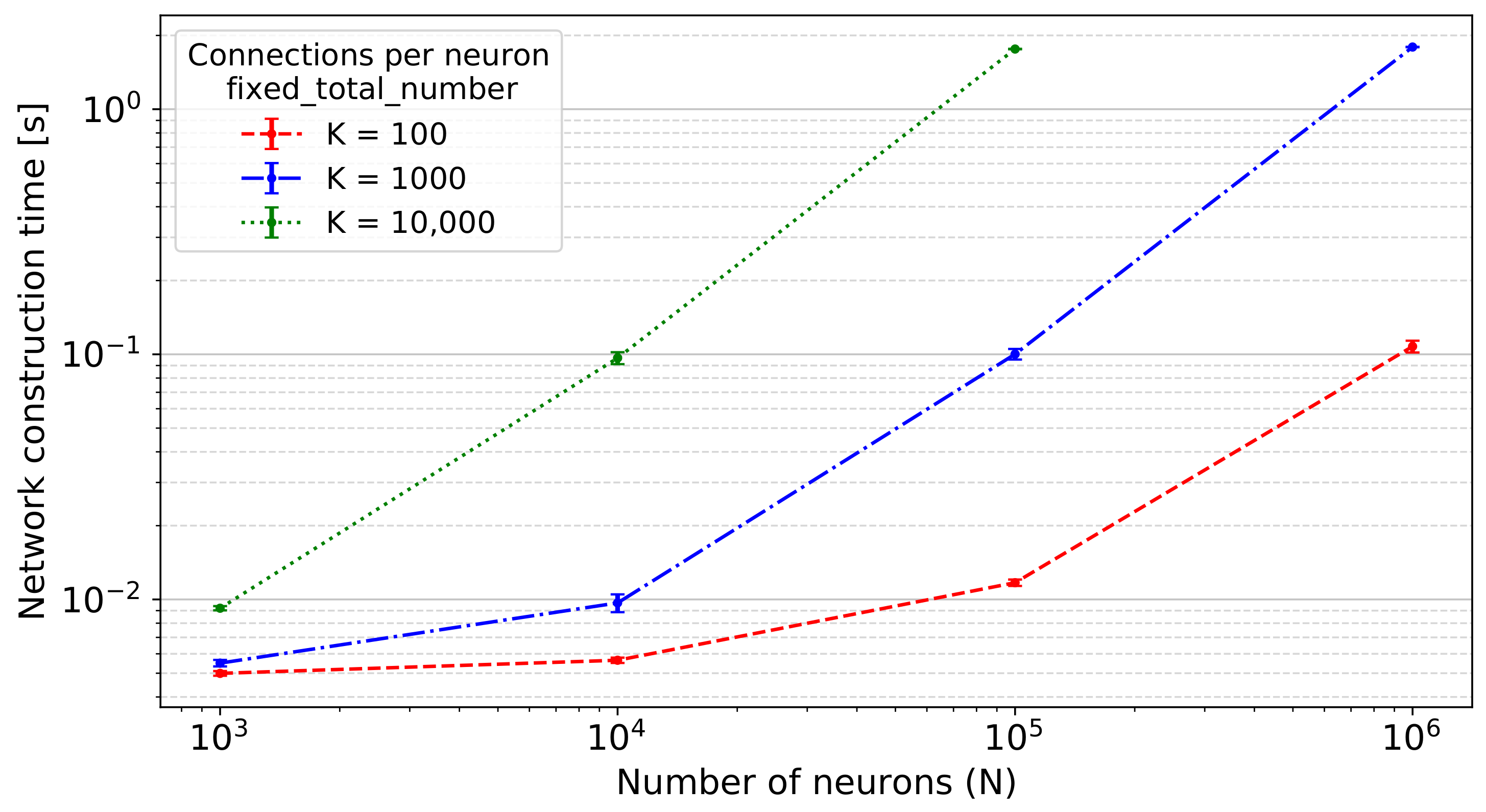
  • Random, fixed total number with multapses (fixed_total_number):
    s = s 0 + rand ( N sources )
    t = t 0 + rand ( N targets )
    where pairs of sources and targets are sampled until the specified total number of connections N newconns is reached.
If the indexes of source or target nodes are not consecutive but are explicitly given by an array, the above formulas are used to derive the indexes of the array elements from which to extract the node indexes. Weights and delays can have identical values for all connections, or be specified for each connection by an array having a size equal to the number of connections or be randomly distributed according to a given probability distribution. In the latter case, the pseudo-random numbers are generated using the cuRAND library (https://developer.nvidia.com/curand, accessed on 14 August 2023). The delays are then converted to integer numbers expressed in units of the computation time step by dividing their values, expressed in milliseconds, by the duration of the computation time step, and rounding the result to an integer. The minimal delay that is permitted is one computation time step [22]. Thus, if the result is less than 1, the delay is set to 1 in time step units.

2.2. Data Structures Used for Connections

In order to efficiently manage the spike transmission in the presence of delays, the connections must be organized in an appropriate way. To this end, the algorithm divides the connections into groups so that connections from the same group share the same source node and the same delay. This arrangement is needed for the spike delivery algorithm, which is described in the next section. The algorithm achieves this by hierarchically using two sorting keys: the index of the source node as the first key and the delay as the second. Since the connections are created dynamically, their initial order is arbitrary. Therefore, we order connections in a stage that follows network construction and that precedes the simulation called calibration phase (for a definition of the simulation phases, see Section 2.6). The sorting algorithm is an extension of radix sort [23] applied to an array organized in blocks based on the implementation available in the CUB library (https://nvlabs.github.io/cub, accessed on 14 August 2023). Once the connections are sorted, their groups must be adequately indexed so that when a neuron emits a spike, the code has quick access to the groups of connections outgoing from this neuron and to their delays. This indexing is carried out in parallel using CUDA kernels on connection blocks with one CUDA thread for each connection. The connection index extracts the source node index and the connection delay. If one of these two values differs from those of the previous connection, it means that the current connection is the first of a connection group. We use this criterion to count the number of connection groups per source node, G i , and to find the position of each connection group in the connection blocks. The next step constructs for each source node an array of size equal to the number of groups of outgoing connections containing the global indexes of the first connections of each group. Since allocating a separate array for each node would be a time-consuming operation, we concatenate all arrays into a single one-dimensional array. The starting position p i of the sub-array corresponding to a given source node i can be evaluated using the cumulative sum of G i as follows:
p i = j = 0 i 1 G j i = 1 , , N nodes and p 0 = 0
where N nodes is the total number of nodes in the network.

2.3. The Spike Buffer

The simulation algorithm employs a buffer of outgoing spikes for each neuron in the network to manage connection delays [9,13]. Each spike object is composed of three parameters: a time index, a connection group index, and a multiplicity (i.e., the number of physical spikes emitted by a network node in a single time step). The spike buffer has the structure of a queue into which the spikes emitted by the neuron are inserted. Whenever a spike is emitted from the neuron, it is buffered, and both its time index and its connection-group index are initialized to zero. At each simulation time step, the time indexes of all the spikes are increased by one unit. When the time index of a spike matches the delay of the connection group indicated by its connection group index, the spike is fed into a global array called spike array, and its connection group index is incremented by one unit to point to the next connection group in terms of delay. In the spike array, each spike is represented by the source node index, the connection group index, and the multiplicity. The spikes are delivered in parallel to the target nodes using a CUDA kernel with one CUDA thread for each connection of each connection group inserted in the spike array.

2.4. Models Used for Performance Evaluation

This present work evaluates the performance of the proposed approach on two network models: a cortical microcircuit and a simple network model of two neuron populations. The models are depicted schematically in Figure 2. The microcircuit model of Potjans and Diesmann [24] represents a 1 mm 2 patch of early sensory cortex at the biological plausible density of neurons and synapses. The full-scale model comprises four cortical layers (L2/3, L4, L5, and L6) and consists of about 77,000 current-based leaky integrate-and-fire model neurons, which are organized into one excitatory and one inhibitory population per layer. These eight neuron populations are recurrently connected by about 300 million synapses with exponentially decaying postsynaptic currents; the connection probabilities are derived from anatomical and electrophysiological measurements. The connection rule used is fixed_total_number with autapses and multapses allowed. The dynamics of the membrane potentials and synaptic currents are integrated using the exact integration method proposed by Rotter and Diesmann [25], and the membrane potential of the neurons of every population are initialized from a normal distribution with mean and standard deviation optimized from the neuron population as in [26]. This approach avoids transients at the beginning of the simulation. Signals originating from outside of the local circuitry, i.e., from other cortical areas and the thalamus, can be approximated with Poisson-distributed spike input or DC current input. Tables 1–4 of [27] (see fixed total number models) contain a detailed model description and report the values of the parameters. The model explains the experimentally observed cell-type and layer-specific firing statistics, and it has been used in the past both as a building block for larger models (e.g., [28]) and as a benchmark for several validation studies [9,17,26,29,30,31,32].
The second model is designed for testing the scaling performance of the network construction by changing the number of neurons and the number of connections in the network across biologically relevant ranges for different connection rules (see Section 2.1; autapses and multapses allowed). The model consists of two equally sized neuron populations, which are recurrently connected to themselves and to each other in four nestgpu.Connect() calls. The total number of neurons in the network is N (i.e., N / 2 per population), and the target total number of connections is N × K connections, where K is the target number of connections per neuron. Dependent on the connection rule used, the instantiated networks may exhibit small deviations from the following target values:
  • fixed_total_number:
    The total number of connections used in each connect call is set to N × K / 4 .
  • fixed_indegree:
    The in-degree used in each connect call is set to K / 2 .
  • fixed_outdegree:
    The out-degree used in each connect call is set to K / 2 .
The network uses Izhikevich neurons [33], but the studied scaling behavior is independent of the neuron model as well as the neuron, connection, and simulation parameters. Indeed, the only parameters that have an impact on this scaling experiment are the total number of neurons and the number of connections per neuron (i.e., N and K).

2.5. Hardware and Software of Performance Evaluation

As a reference, we implement the proposed method for generating connections directly in GPU memory in the GPU version of the simulation code NEST. In the following, NEST GPU (onboard) refers to the new algorithm in which the connections are created directly in GPU memory, while NEST GPU (offboard) indicates the previous algorithm, which first generates the network in CPU memory and subsequently copies the network structure into the GPU as demonstrated in [9,13]. For a quantitative comparison to other established codes, we use the CPU version of NEST [1] (version 3.3 [34]) and the GPU code generator GeNN [6] (version 4.8.0 (https://github.com/genn-team/genn/releases/tag/4.8.0, accessed on 14 August 2023)).
We evaluate the performance of the alternative codes on four systems equipped with NVIDIA GPUs of different generations and main application areas: two compute clusters, JUSUF [35] and JURECA-DC [36], both using CUDA version 11.3 and equipped with the data center GPUs V100 and A100, respectively, and two workstations with the consumer GPUs RTX 2080 Ti, with CUDA version 11.7 and RTX 4090 with CUDA version 11.4. The NEST GPU and GeNN simulations discussed in this work each employ a single GPU card, both because the novel network construction method developed for NEST GPU is limited to single-GPU simulations and also because all the simulation systems employed have enough GPU memory to simulate the models previously described using a single GPU card. The CPU simulations use a single compute node of the HPC cluster JURECA-DC and exploit its 128 cores via 8 MPI processes each running 16 threads. Table 1 shows the specifications of these three systems.
For the network models, their specific implementations were taken from the original source for each simulator in the case of the cortical microcircuit model. In particular, both NEST (https://github.com/nest/nest-simulator, accessed on 14 August 2023) and NEST GPU (https://github.com/nest/nest-gpu, accessed on 14 August 2023) provide example implementations of the cortical microcircuit model inside their respective source code repositories. Additionally, GeNN provides their own implementation of the microcircuit along with the data used for their PyGeNN publication [17] in the corresponding publicly available GitHub repository (https://github.com/BrainsOnBoard/pygenn_paper, accessed on 14 August 2023). Furthermore, to correctly compare the performance of the simulation, we adapt the existing scripts so that the overall behavior remains the same. In particular, we disabled spike recordings and we enabled optimized initialization of membrane potentials as in [26].
The second model presented in Section 2.4 is implemented for NEST GPU (onboard), and different connection rules can be chosen for the simulation. See the Data Availability Statement for further details on how to access the specific model versions used in this publication.

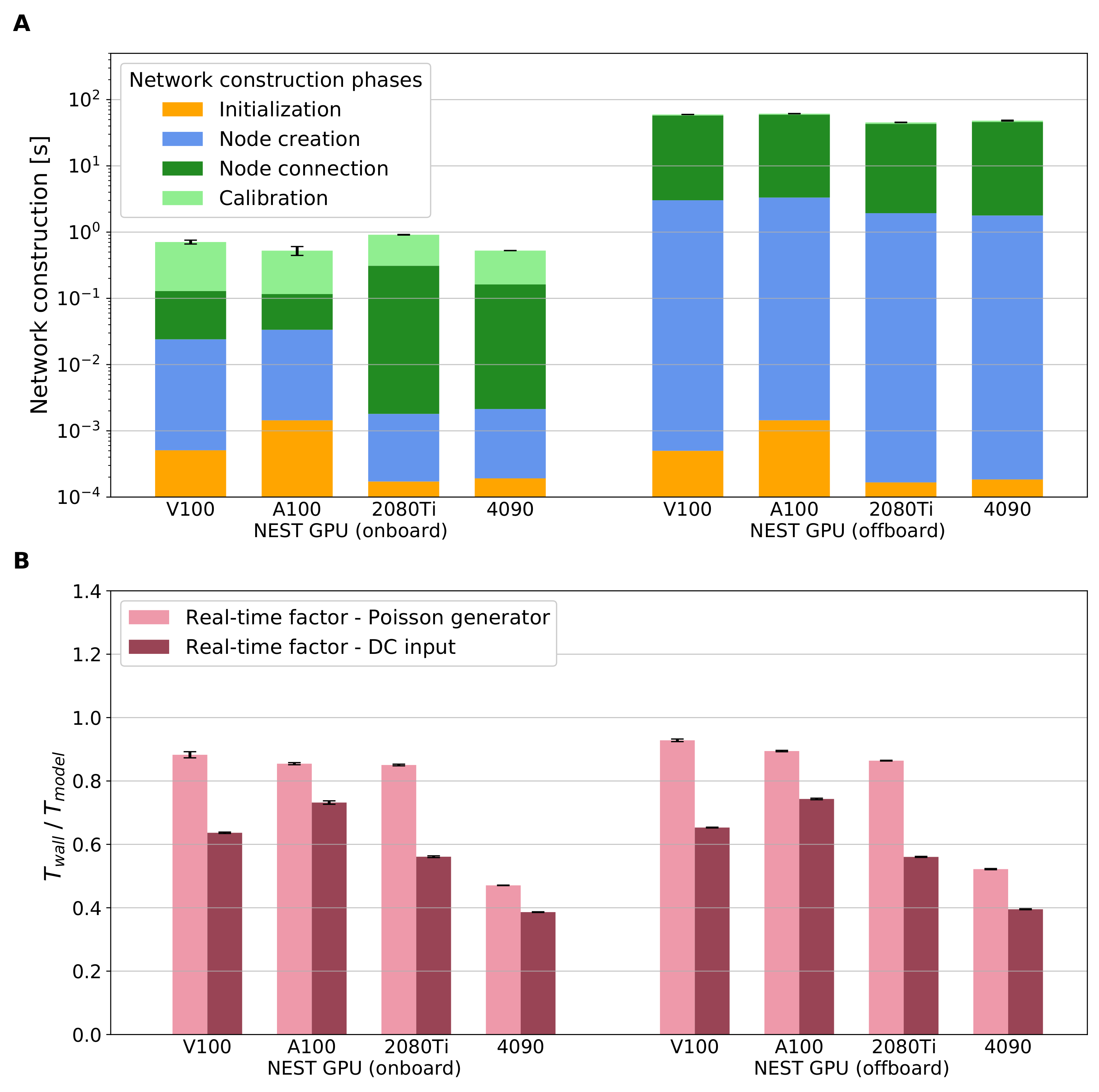
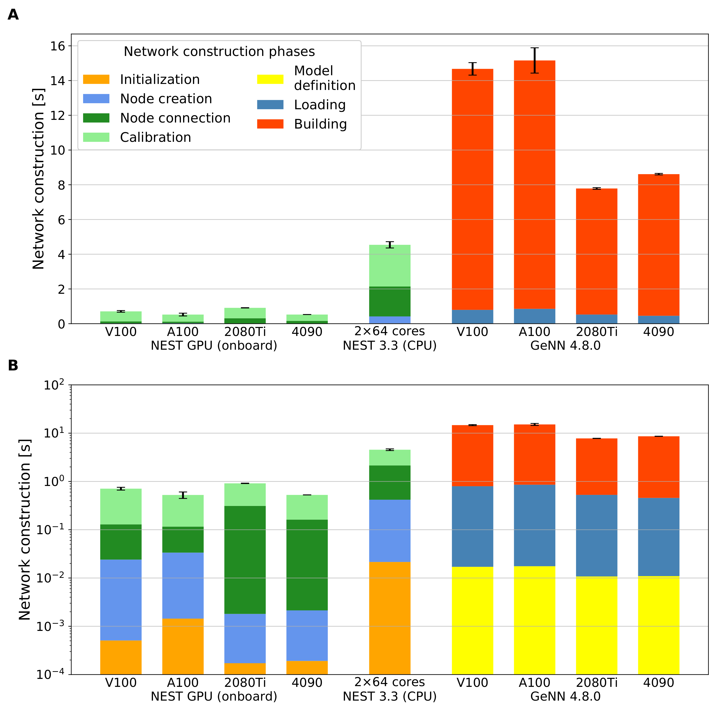
2.6. Simulation Phases

On the coarse level, we divide a network simulation into two successive phases: network construction and simulation. The network construction phase encompasses all steps until the actual simulation loop starts. To assess different contributions to the network construction, we further divide this phase into stages. The consecutively executed stages in the NEST implementations (both CPU and GPU versions) follow the same pattern as follows:
  • Initialization is a setup phase in the Python script for preparing both model and simulator by importing modules, instantiating a class, or setting parameters, etc.
    •    import nestgpu
  • Node creation instantiates all the neurons and devices of the model.
    •    nestgpu.Create()
  • Node connection instantiates the connections among network nodes.
    •    nestgpu.Connect()
  • Calibration is a preparation phase that orders the connections and initializes data structures for the spike buffers and the spike arrays just before the state propagation begins. In the CPU code, the pre-synaptic connection infrastructure is set up here. This stage can be triggered by simulating just one time step h.
    •    nestgpu.Simulate(h)
    Previously, the calibration phase of NEST GPU was used to finish moving data to the GPU memory and instantiate additional data structures like the spike buffer (cf. Section 2.3). Now, as no data transfer is needed and connection sorting is carried out instead (cf. Section 2.2), the calibration phase is now conceptually closer to the operations carried out in the CPU version of NEST [37].
In GeNN, the network construction is decomposed as follows:
  • Model definition defines neurons and devices and synapses of the network model.
    •    from pygenn import genn_model
    •    model = genn_model.GeNNModel()
    •    model.add_neuron_population()
  • Building generates and compiles the simulation code.
    •    model.build()
  • Loading allocates memory and instantiates the network on the GPU.
    •    model.load()
Timers at the level of the Python interface assess the performance of the three different simulation engines. This has the advantage of being agnostic to the implementation details of each stage at the kernel level, including any overhead of data conversion required by the C++ API, and close to the actual time perceived by the user.

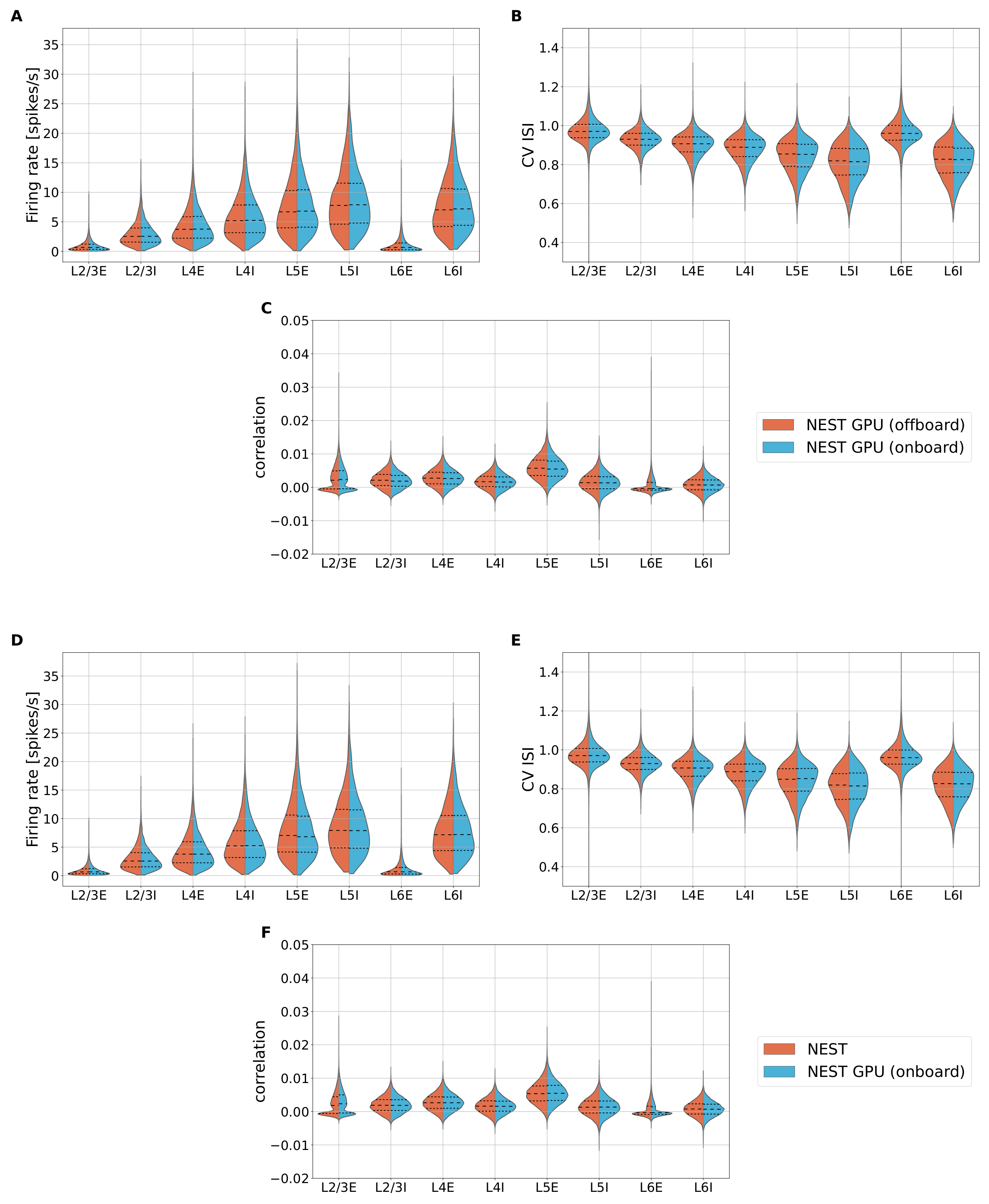
2.7. Validation of the Proposed Network Construction Method

The generation of random numbers for the probabilistic connection rules differs between the previous and the novel approach for network construction in NEST GPU. This means that the connectivity resulting from the same rule with the same parameters is not identical but only matches on a statistical level. It is, therefore, necessary to determine that the network dynamics is qualitatively preserved.
Using the cortical microcircuit model, we validate the novel method against the previous one using a statistical analysis of the simulated spiking activity data. To this end, we apply a similar validation procedure to that proposed in [9,13], where the GPU version of NEST was compared to the CPU version as a reference. We follow the example of [26,27,29,32] and compute for each of the eight neuron populations three statistical distributions to characterize the spiking activity as follows:
  • Time-averaged firing rate for each neuron;
  • Coefficient of variation of inter-spike intervals (CV ISI);
  • Pairwise Pearson correlation of the spike trains obtained from a subset of 200 neurons for each population.
These distributions are then compared for the two different approaches for network construction, as detailed in Appendix B.

3. Results

This section evaluates the performance of the proposed method for generating connections directly in GPU memory using the reference implementation NEST GPU (onboard). For the cortical microcircuit model, we compare the network construction time and the real-time factor of the simulations obtained with the novel method to NEST GPU (offboard) (i.e., the simulator version employing the previous algorithm of instantiating the connections first on the CPU), the CPU version of the simulator NEST [1] and the code-generation based simulator GeNN [6].
With the two-population network model, we assess the network construction time upon scaling the number of neurons and the number of connections per neuron. Refer to Section 2.4 for details on the network models.

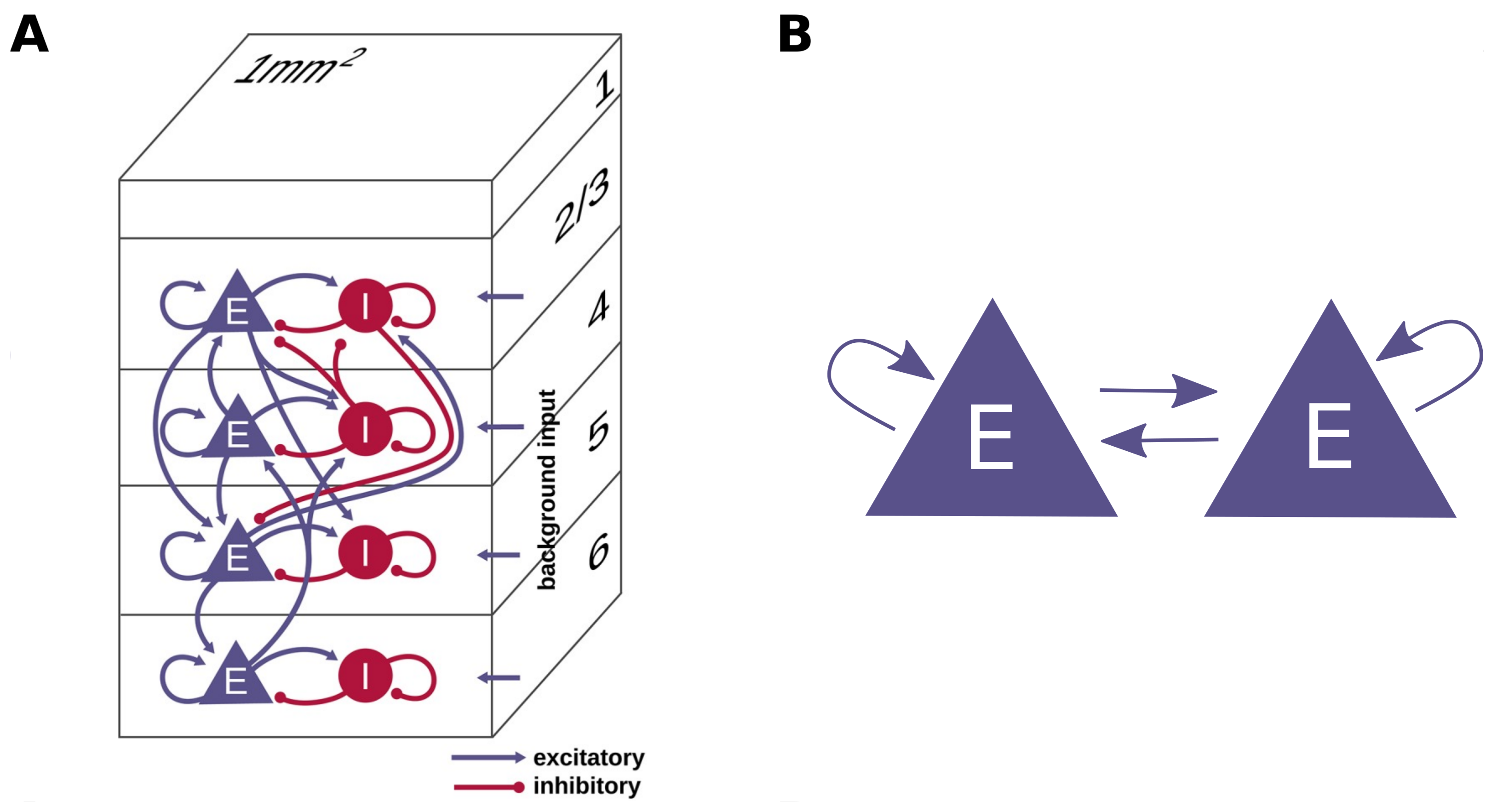
3.1. Cortical Microcircuit Model

Figure 3 directly compares the two approaches for network construction implemented in NEST GPU, i.e., onboard and offboard, in terms of the network construction time (panel A) and the real-time factor obtained using a simulation of the network dynamics (panel B). Panel A shows that the novel method for network construction enables a speed up by two orders of magnitude with respect to the previous network construction algorithm. The overhead of the offboard method (used in [9,13]) transferring the network from CPU to GPU becomes obsolete with the proposed approach to generate the connections directly on the GPU. Moreover, the onboard version shows lower network construction times across all hardware configurations without compromising the simulation times (panel B). An additional detail to take note of with the novel algorithm is that the calibration phase is now by far the longest compared to the node creation and node connection (3–5 times longer, depending on the hardware used). However, this is only due to the fact that both the creation and connection phases are now only used to instantiate data structures in GPU memory, whereas the calibration phase takes charge of the connection sorting as described in Section 2.2. Both versions have real-time factors of less than one second (sub-real-time simulation), thus showing also an improvement in the simulation time compared to the results of [9] obtained with the prototype NeuronGPU library. Additionally, in some cases, it is possible to see a small improvement when simulating using the novel network construction approach due to some code optimization related to the simulation phase. While the network construction times are independent of the choice of external drive, the DC input as expected leads to faster simulations of the network dynamics compared to the Poisson generators. Comparing the different hardware configuration, the smallest real-time factor obtained with NEST GPU (onboard) is achieved with DC input on the latest consumer GPU RTX 4090, 0.386 ( 0.001 ) (mean (standard deviation)). The respective result for Poisson input is 0.4707 ( 0.0008 ) . For completeness, we also measure the real-time factor of NEST and GeNN simulations using the same framework used for Figure 3B. These results are shown in Table 2, Table 3 and Table 4 and depicted in Appendix C.
Figure 4 compares the network construction times of the full-scale cortical microcircuit model obtained using NEST GPU (onboard), NEST 3.3, and GeNN 4.8.0 on different hardware configurations; for details on the hardware and software configurations, see Section 2.5. The settings are the same as in Figure 3. While panel A resolves the contributions of the different stages (defined in Section 2.6) using a linear y-axis, panel B shows the same data with logarithmic y-axis to facilitate a comparison of the absolute numbers. As mentioned in Section 2.4, the external input to the cortical microcircuit implementations in both the CPU and GPU versions of NEST can be provided via either generators of Poisson signals or DC input. We run simulations comparing both approaches. However, Figure 4 only shows the results for the case of Poisson generators because the network construction times with DC input are similar. GeNN, in contrast, mimics the incoming Poisson spike trains via a current directly applied to each neuron. Both NEST GPU (onboard) and GeNN (without the building phase) achieve fast network construction times of less than a second. The fastest overall network construction takes 0.499 ( 0.10 )  s, as measured with NEST GPU (onboard) using DC input on the A100 GPU, the data center GPU of the latest architecture tested. The time measured using the RTX 4090 is also compatible with the A100 result; the measured times with the V100 and the consumer GPU RTX 2080 Ti are also close. Table 2, Table 3 and Table 4 provide the measured values for reference.
Hitherto, we discussed the performance for both network construction and simulation of NEST GPU (onboard) compared to NEST GPU (offboard), NEST, and GeNN. Turning on the statistical analysis of the simulated activity, data show good agreement between NEST GPU (offboard) and NEST GPU (onboard) as well as between NEST GPU (onboard) and NEST 3.3. That means that differences between the compared simulator versions are of the same order as the fluctuations due to the choice of different seeds in either of the codes (see Section 2.7 and Appendix B). The novel approach constructs the network model in around half a second, whereas the same task using the previous network construction method took around a minute. In this validation process, we, therefore, experience a 15% reduction in the overall time to solution when obtaining the simulated activity of 600 s of biological time from NEST GPU (onboard) with respect to NEST GPU (offboard). More details on the time needed to perform this study are reported in the Appendix B.

3.2. Two-Population Network

The two-population network described in Section 2.4 is designed to evaluate the scaling performance of the proposed network construction method. To this end, we perform simulations on NEST GPU (onboard) varying the number of neurons and the number of connections per neuron. The scaling performance of NEST GPU (offboard) has been evaluated on [9] for a balanced network model. We opted for a total number of neurons in the network (N) ranging from 1000 to 1,000,000 and a target number of connections per neuron (K) ranging from 100 to 10,000.
To enable the largest networks, benchmarks are performed on the JURECA-DC cluster, which is equipped with the GPUs with the largest GPU memory (i.e., the NVIDIA A100 with 40 GB) among the systems described in Table 1. Figure 5 shows the network construction times using the fixed_total_number connection rule and ranging the number of neurons and connections per neuron. The performance obtained using the fixed_indegree and fixed_outdegree connection rules are totally compatible with the ones shown in this figure, and the respective plots are available in Appendix D for completeness.
As can be seen, the value of network construction time for the network with 10 6 neurons and 10 4 connections per neuron is not shown because of the lack of GPU memory. Using an NVIDIA A100 GPU, we can, thus, say that this method enables the construction of networks with up to an order of magnitude of 10 9 connections. The largest network tested on this GPU comprised 3 × 10 5 neurons with K = 10 , 000 connections per neuron (data not shown).

4. Discussion

It takes less than a second to generate the network of the cortical microcircuit model [24] with the GPU version of NEST using our proposed dynamic approach for creating connections directly in GPU memory on any GPU device tested. That is two orders of magnitude faster than the previous algorithm, which instantiates the connections first on the CPU and copies them from RAM to GPU memory just before the simulation starts (Figure 3). The reported network construction times are also shorter compared to the CPU version of NEST and the code generation framework GeNN (Figure 4); if code generation and compilation are not required in GeNN, the results of NEST GPU and GeNN are compatible. The time to simulate the network dynamics after network construction is not compromised by the novel approach.
The latest data center and consumer GPUs (i.e., A100 and RTX 4090, respectively) show the fastest network constructions as expected, approximately 0.5 s. We observe the shortest simulation times on the RTX 4090 and attribute this result to the fact that the kernel design of NEST GPU particularly benefits from the high clock speeds of this device (cf. Section 2.5). Contrary to expectation, our simulations with DC input on the A100 are slower compared to the V100 although the former has higher clock speeds; an investigation of this observation is left for future work.
For models of the size of the cortical microcircuit, the novel approach renders the contribution of the network construction phase to the absolute wall-clock time negligible, even for short simulation durations. Further performance optimizations should preferentially target the simulation phase. Our result that GeNN currently simulates faster than NEST GPU indicates that there is room for improvement, which could possibly be exploited via further parallelizations of the simulation kernel.
The evaluation of the scaling performance with the two-population network on the A100 shows that the network construction time is dominated by the total number of connections (i.e., N × K , Figure 5) and mostly independent of the connection rule used. The maximum network size that can be simulated depends on the GPU memory of the card employed for the simulation. Future generation GPU cards with more memory available will enable the construction of larger or denser networks of spiking neurons and, at the same time, give reasons to expect further performance improvements with novel architectures and the possibility of an even higher degree of parallelism. Nonetheless, this conclusion is affected by the structure of the connection objects, as each object contains multiple data like the weight and the delay (cf. Section 2.2); when using natural connection density, GPU memory would be consequently filled up faster. However, if one considers simple connection objects like the ones used in weightless neural networks such as the Ring Probabilistic Logic Neural Networks discussed in [38], the maximum network size would naturally increase. The novel approach is currently limited to simulations on a single GPU, and future work is required to extend the algorithm to employ multiple GPUs as achieved with the previous algorithm [13].
Further improvements to the library may also expand upon the available connection rules and more flexible control via the user interface. At present, the pairwise Bernoulli connection routine [21] is not available; this is because the onboard construction method requires a precise number of connections that must be allocated at once in order to not waste any GPU memory. The pairwise Bernoulli connection routine implies that this number is not known; hence, additional heuristics would be required to optimize memory usage. Autapses and multapses are currently always allowed in NEST GPU; therefore, another useful addition would be the possibility to prohibit them (for example, using a flag as in the CPU version of NEST).
In conclusion, we propose a novel algorithm for network construction, which dynamically creates the network exploiting the high degree of parallelism of GPU devices. It enables short network construction times comparable to code generation methods and the advantageous flexibility of run-time instantiation of the network. This optimized method makes the contribution of the network construction phase in network simulations marginal, even when simulating highly-connected large-scale networks. As discussed in [39], this is especially interesting for parameter scan applications, where a high volume of simulations needs to be tested, and any additional contribution to the overall execution time of each test aggregates considerably and slows down the exploration process. Future work can investigate the extension of this algorithm for multi-GPU simulations, incorporate further connection rules, and optimize the simulation kernel to enable the fast network construction and simulation of large networks approaching the size of the human brain.

Author Contributions

Conceptualization, B.G., J.V., G.T., E.P., J.S. (Jonas Stapmanns), V.F., P.S.P., A.M. and J.S. (Johanna Senk); methodology, B.G., J.V., G.T., E.P., J.S. (Jonas Stapmanns), P.S.P., A.M. and J.S. (Johanna Senk); software, B.G., J.V., G.T., J.S. (Jonas Stapmanns) and J.S. (Johanna Senk); investigation, formal analysis, visualization, validation, and data curation, B.G., J.V., G.T. and J.S. (Johanna Senk); resources, funding acquisition and supervision, B.G., P.S.P., A.M. and J.S. (Johanna Senk); writing—original draft preparation, B.G., J.V., G.T. and J.S. (Johanna Senk); writing—review and editing, B.G., J.V., G.T., E.P., J.S. (Jonas Stapmanns), V.F., P.S.P., A.M. and J.S. (Johanna Senk); project administration, B.G. and J.S. (Johanna Senk). All authors have read and agreed to the published version of the manuscript.

Funding

This project has received funding from the European Union’s Horizon 2020 Framework Programme for Research and Innovation under Specific Grant Agreement No. 945539 (Human Brain Project SGA3), the Initiative and Networking Fund of the Helmholtz Association in the framework of the Helmholtz Metadata Collaboration project call (ZT-I-PF-3-026), and the Joint Lab “Supercomputing and Modeling for the Human Brain”, the Italian PNRR MUR project PE0000013-FAIR CUP I53C22001400006, funded by NextGenerationEU.

Institutional Review Board Statement

Not applicable.

Informed Consent Statement

Not applicable.

Data Availability Statement

The code to reproduce all figures of this manuscript is publicly available at Zenodo: https://doi.org/10.5281/zenodo.7744238, accessed on 14 August 2023. The versions of NEST GPU employed in this work are available on GitHub (https://github.com/nest/nest-gpu, accessed on 14 August 2023) via the git tags nest-gpu_onboard and nest-gpu_offboard.

Acknowledgments

The authors gratefully acknowledge the computing time granted by the JARA Vergabegremium and provided on the JARA Partition part of the supercomputer JURECA at Forschungszentrum Jülich (computation grant JINB33) and the use of Fenix Infrastructure resources, which are partially funded from the European Union’s Horizon 2020 research and innovation programme through the ICEI project under the Grant Agreement No. 800858. The authors further thank the INFN APE Parallel/Distributed Computing laboratory and INM-6/IAS-6. Part of the work was performed while Gianmarco Tiddia enjoyed a scientific stay at INM-6/IAS-6 in the period from 21st of September 2022 to 28th of March 2023. The authors would also like to thank Markus Diesmann for the detailed comments on the manuscript and Andrea Bosin, Fabrizio Muredda, and Giovanni Serra for their support in the use of the RTX 4090 GPU.

Conflicts of Interest

The authors declare no conflict of interest. The sponsors had no role in the design, execution, interpretation, or writing of this study.

Appendix A. Block Sorting

The following appendix describes the block sorting algorithm employed in the network construction phase of the simulation and particularly when organizing connections among the nodes of the network.
Figure A1. The COPASS block-sort algorithm. (A) Unsorted array, divided in blocks (subarrays). Each element of the array is represented as a blue bar. The vertical solid lines represent the division in subarrays. (B) Each subarray is sorted using the underlying sorting algorithm. (C) The subarrays are divided in two partitions each using a common threshold, t, in such a way that the total size of the left partitions (represented in red) is equal to the size of the first block. (D) The left partitions are copied to the auxiliary array. (E) The right partitions are shifted to the right, and the auxiliary array is copied to the first block. (F) The auxiliary array is sorted. The procedure from (C) to (E) is then repeated on the new subarrays, delimited by the green dashed lines, in order to extract and sort the second block, and so on, until the last block.
Applsci 13 09598 g0a1

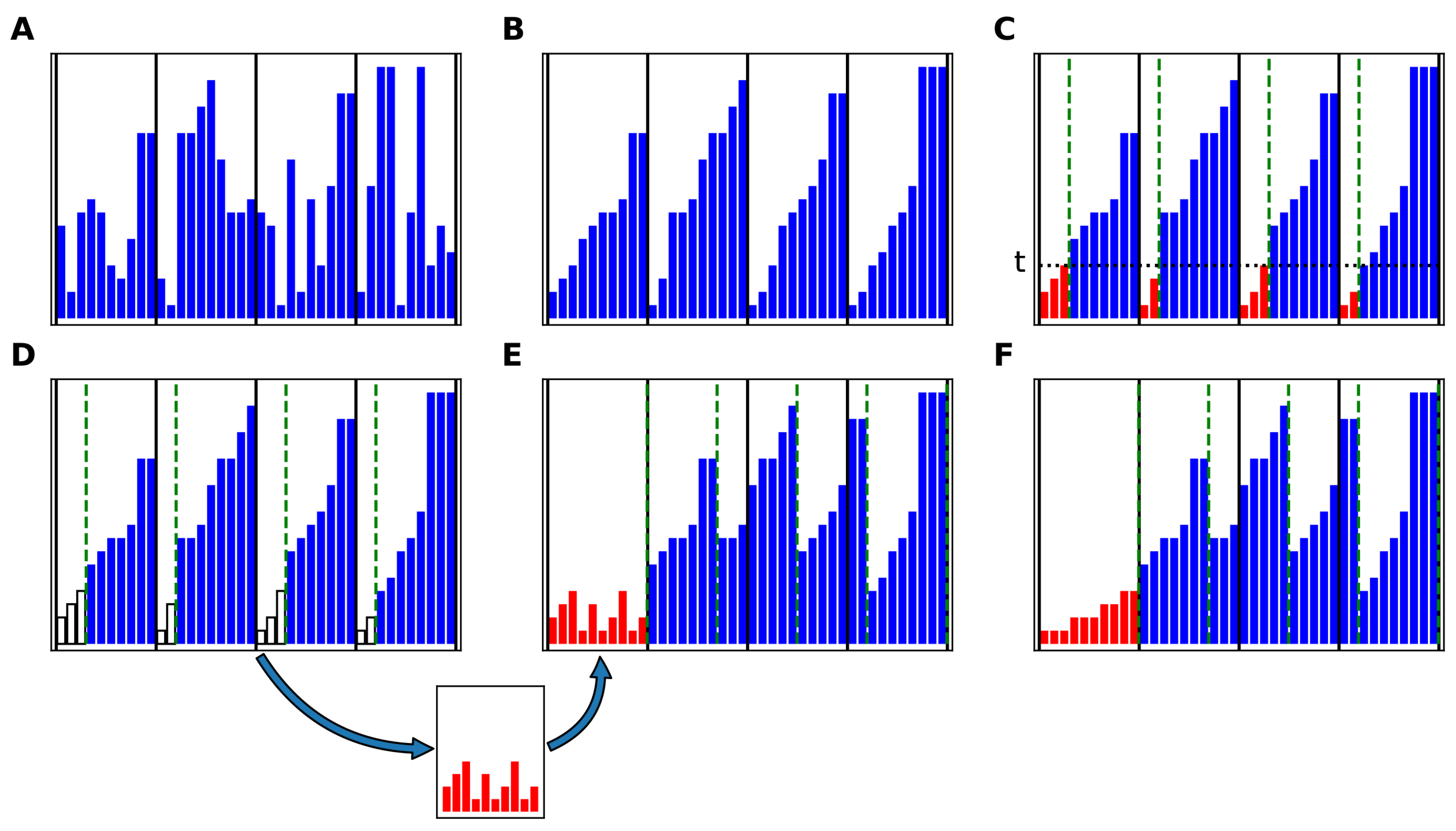
Appendix A.1. The COPASS (Constrained Partition of Sorted Subarrays) Block-Sort Algorithm

Given a real-number array A divided in k blocks (subarrays) S i , j of sizes N i
A = S 0 , 0 , , S 0 , N 0 , S 1 , 0 , , S 1 , N 1 , S k 1 , 0 , , S k 1 , N k 1
S i , j R i = 0 , , k 1 j = 0 , , N i
The aim of the COPASS block-sort algorithm is to perform an in-place sort of A maintaining its block structure. This algorithm relies on another algorithm for sorting each block. It should be noted that the subarrays do not need to be stored in contiguous locations in memory. The COPASS block-sort algorithm is illustrated in Figure A1. The k subarrays are sorted using the underlying sorting algorithm (Figure A1B). Each sorted subarray is divided in two partitions using the COPASS algorithm, described in the next sections, in such a way that all the elements of the left partitions (represented in red) are smaller than or equal to a proper common threshold, t, while all the elements of the right partitions are greater than or equal to t, and the total number of elements of the left partitions is equal to the size of the first block, N 0 (Figure A1C). The elements of the left partitions are copied to the auxiliary array (Figure A1D). The right partitions are shifted to the right, leaving the first block free, and the auxiliary array is copied to the first block (Figure A1E). The auxiliary array is sorted (Figure A1F). The whole procedure is then repeated for extracting the second block, using the logical subarrays delimited by the green dashed lines in Figure A1F, and so on, until the last block is extracted. The maximum size of the auxiliary array is equal to the size of the largest block, i.e.,
m max = max i { N i }
The auxiliary storage requirement of the COPASS block-sort algorithm is the largest between the auxiliary storage requirement of the underlying sorting algorithm for an array of size m max and the auxiliary array storage requirement. This requirement can be reduced by dividing A in a large number of small blocks.

Appendix A.2. The COPASS Partition Algorithm

Given a set of k real-number arrays S i , j (here called subarrays) of sizes N i
S i , j R i = 0 , , k 1 j = 0 , , N i
each sorted in ascending order
S i , j S i , l for j l
and a positive integer m < i , j S i , j , the purpose of this algorithm is to find a threshold t and k non-negative integers m i such that
S i , j t for j < m i
S i , j t for j m i
i m i = m       
We will call left partitions the subarrays of size m i
S i , j j = 0 , , m i 1
and right partitions the complementary subarrays
S i , j j = m i , , N i 1
The basic idea of the algorithm is to start from an initial interval [ t ¯ 0 , t ¯ 0 ] , such that t ¯ 0 t t ¯ 0 , and to proceed iteratively, shrinking the interval and ensuring that the condition
t ¯ s t t ¯ s
is satisfied at each iteration index s, until either t ¯ s or t ¯ s is equal to t. For this purpose, for each iteration index s, we define m ¯ i , s as the number of the elements of the subarray S i , j that are smaller than or equal to t ¯ s , i.e., the cardinality of the set of integers j such that S i , j t ¯ s
m ¯ i , s = card { j : S i , j t ¯ s }
and m ¯ i , s as the number of elements that are strictly smaller than t ¯ s
m ¯ i , s = card { j : S i , j < t ¯ s }
Since the subarrays S i , j are sorted, and m ¯ i , s and m ¯ i , s can be computed through a binary search algorithm. In a parallel implementation, their values can be evaluated for all i = 0 , , k 1 by performing the binary searches in parallel on the k subarrays. As an initial condition, we set
t ¯ 0 = min ( S i , j ) 1
t ¯ 0 = max ( S i , j ) + 1
From Equations (A12) and (A13), it follows that
m ¯ i , 0 = 0
m ¯ i , 0 = N i
and
i m ¯ i , 0 < m < i m ¯ i , 0
We proceed iteratively to evaluate the values of t ¯ s + 1 , t ¯ s + 1 , m ¯ i , s + 1 and m ¯ i , s + 1 for the iteration index s + 1 from their values at the previous iteration index s. Assume that the condition
i m ¯ i , s < m < i m ¯ i , s
is satisfied for the iteration index s. The iterations are carried on only if m ¯ i , s m ¯ i , s > 1 for at least one index i, i.e.,
i : m ¯ i , s m ¯ i , s > 1
If the latter condition is not met, the iterations are concluded, and a solution is found as described in Appendix A.3. Otherwise, if Equation (A20) is satisfied, let
l s = arg max i { m ¯ i , s m ¯ i , s }
m ˜ s = m ¯ l s , s + m ¯ l s , s 2
t ˜ s = S l s , m ˜ s
where x represents the integer part of x. Since m ¯ l s , s m ¯ l s , s > 1 , clearly m ¯ l s , s < m ˜ s < m ¯ l s , s , and from Equations (A12) and (A13)
t ¯ s < t ˜ s < t ¯ s
Let
μ ¯ i , s = card { j : S i , j t ˜ s }
μ ¯ i , s = card { j : S i , j < t ˜ s }
From the latter equations and from Equations (A12) and (A13), it follows that
m ¯ i , s μ ¯ i , s μ ¯ i , s m ¯ i , s
for all i, and thus,
i m ¯ i , s i μ ¯ i , s i μ ¯ i , s i m ¯ i , s
The three following cases are possible:
  • Case 1
    i μ ¯ i , s m i μ ¯ i , s
    In this case, t = t ˜ s . The iteration is concluded, and the partition sizes m i are computed using the procedure described in Appendix A.4.
  • Case 2
    i m ¯ i , s < m < i μ ¯ i , s
    In this case, we set
    m ¯ i , s + 1 = m ¯ i , s t ¯ s + 1 = t ¯ s
    m ¯ i , s + 1 = μ ¯ i , s t ¯ s + 1 = t ˜ s
    and continue with the next iteration. Equations (A30)–(A32) ensure that the condition of Equation (A19) is satisfied for the next iteration index s + 1 .
  • Case 3
    i μ ¯ i , s < m < i m ¯ i , s
    In this case, we set
    m ¯ i , s + 1 = μ ¯ i , s t ¯ s + 1 = t ˜ s
    m ¯ i , s + 1 = m ¯ i , s t ¯ s + 1 = t ¯ s
    and continue with the next iteration. Equations (A33)–(35) ensure that the condition of Equation (A19) is satisfied for the next iteration index s + 1 .

Appendix A.3. The COPASS Partition Last Step, Case 1

This final step is carried out at the end of the iterations when the following condition is met:
m ¯ i , s m ¯ i , s 1 i
Consider the set of the ordered pairs ( S i , m ¯ i , s , i ) such that m ¯ i , s is equal to m ¯ i , s + 1
C = { ( S i , m ¯ i , s , i ) : m ¯ i , s = m ¯ i , s + 1 }
We sort them in ascending order of S i , m ¯ i , s values
C ˜ = sort ( C )
Let d be the difference
d = m i m ¯ i , s
and D the set of the first d elements of C ˜
D = { C ˜ 0 , , C ˜ d 1 }
We set the left partition sizes as
m i = m ¯ i , s for ( S i , m ¯ i , s , i ) D
m i = m ¯ i + 1 for ( S i , m ¯ i , s , i ) D
From the latter equation, obviously, the total size of the left partitions will be
m i = m ¯ i , s + d
From Equation (A39), it can be observed that this is equal to m, as requested. Furthermore, since D is sorted, the elements of the left partitions will be smaller than or equal to those of the right partitions.

Appendix A.4. The COPASS Partition Last Step, Case 2

This last step is taken when the condition of Equation (A29) is met. In this case, t = t ˜ s , and from Equations (A25), (A26) and (A29), it follows that
S i , j = t for μ ¯ i , s j μ ¯ i , s
Let d be the difference
d = m i μ ¯ i , s
In order to find a solution for the left partition sizes, m i , we need to find k integers, d i , in the ranges [ 0 , μ ¯ i , s μ ¯ i , s ] , such that their sum is equal to d
i d i = d
μ ¯ i , s d i μ ¯ i , s
and set
m i = μ ¯ i , s + d i
In fact, from Equations (A45), (A46), and (A48), it follows that
i m i = m
as requested, while Equations (A26) and (A44) imply that S i , j is smaller than or equal to t in the left partitions, while it is larger than or equal to t in the right partitions.

Appendix B. Validation Details

As described in Section 2.7, the new method for network construction implemented in NEST GPU needs an in-depth analysis for validating the new version against the previous version of the library. To verify the quality of the results, we collect the spiking activity of the neuron populations of the cortical microcircuit model and compute the three distributions of the spiking activity to be compared, i.e., the average firing rate of the populations, the coefficient of variation of inter-spike intervals (CV ISI), and the pairwise Pearson correlation of the spike trains for each population. The simulations are performed using a time step of 0.1  ms and 500 ms of the network dynamics are simulated before recording the spiking activity to avoid transients. Then, the spiking activity of the subsequent 600 s of network dynamics is recorded to compute the distributions. As shown in [27], this large amount of biological time to be simulated is needed to let the activity statistics converge and, thus, to be able to distinguish the statistic of the activity from random processes. Regarding the performance of such simulations, the real-time factor of NEST GPU with enabled spike recording has only a 1.5 % increase with respect to the performance shown in Figure 3. Figure A2 shows the violin plots of the distributions obtained with the seaborn.violinplot function of the Seaborn [40] Python library. The function computes smoothed distribution through the Kernel Density Estimation method [41,42] with Gaussian kernel, with bandwidth optimized using the Silverman method [43].
Figure A2. Violin plots of the distributions of firing rate (A), CV ISI (B), and Pearson correlation (C) for a simulation for the populations of the cortical microcircuit model using NEST GPU with (sky blue distributions, right) or without (orange distributions, left) the new method for network construction. (DF) Same as (AC), but the orange distributions are obtained using NEST 3.3. Central dashed line represents the median of the distributions, whereas the two dashed lines represent the interquartile range.
Applsci 13 09598 g0a2
The distributions obtained with the two versions of NEST GPU are visually indistinguishable; the distributions of the CPU simulator (version 3.3) are likewise indistinguishable, as previously demonstrated in [9] for the comparison between the previous version of NEST and NeuronGPU, the prototype library of NEST GPU. Additionally, to quantitatively evaluate the difference between the different versions of NEST GPU, we compute the Earth Mover’s Distance (EMD) between the pairs of distributions using the scipy.stats.wasserstein_distance of the SciPy library [44]. More details on this method can be found in [13]. We simulate sets of 100 simulations changing the seed for random number generation. The sets of simulations for the two versions of the NEST GPU library are, thus, pairwise compared, obtaining for each distribution and each population of the model a set of 100 values of EMD, evaluating the difference between the distributions of the two versions of NEST GPU (offboard-onboard). Furthermore, we compute an additional set of simulations for the previous version of NEST GPU to be compared with the other set of the same version (offboard-offboard). This way, we can evaluate the differences that can arise using the same simulator with different seeds for random number generation and compare it with the differences obtained by comparing the two different versions of NEST GPU. Additionally, we performed the same validation to compare NEST and NEST GPU to have a quantitative comparison between the most recent versions of the two simulators, i.e., NEST-NEST GPU (onboard) and NEST-NEST. Figure A3 shows the EMD box plots for all the distributions computed and for all the populations.
Figure A3. Box plots of the Earth Mover’s Distance comparing side by side firing rate (A), CV ISI (B) and Pearson correlation (C) of the two versions of NEST GPU (sky blue boxes, left) and the previous version of NEST GPU using different seeds (orange boxes, right). Panels (DF) are the same as (AC), but distributions of NEST GPU (onboard) and NEST 3.3 are compared. In particular, the comparison between the different simulator is represented by the sky blue boxes on the left, whereas the comparison between two sets of NEST simulations is depicted with the orange boxes. Central line of the box plot represent the median of the distribution, whereas the extension of the boxes is determined by the interquartile range of the distribution formed by the values of EMD of each comparison. Whiskers shows the rest of the distribution as a function of the interquartile range, and dots represent the outliers.
Applsci 13 09598 g0a3
Comparing the box plots in panels A–C reveals very similar distributions in EMD for the two comparisons, meaning that the variability we measure from comparing the two versions is compatible with the one that we have by employing the previous version of NEST GPU using different seeds, ergo the new method does not add variability with respect to simulating the model with the previous version of NEST GPU using different seeds. Similar conclusions can be derived from the comparison between NEST and NEST GPU (onboard) (see panels D–F).
As mentioned before, the real-time factor of NEST GPU marginally increased because of the activation of the spike recording. The overall simulation time of a set of 100 simulations using the novel method for network construction took around 868 min, with less than one minute dedicated to network construction (more precisely, the average time is 0.53  s for a single simulation). A set of simulations obtained using the old method for network construction took around 1020 min, with around 100 min of them related to the network construction phase. This represents a reduction in the network construction time of around 116 times with respect to the previous network construction method.

Appendix C. Additional Data for Cortical Microcircuit Simulations

Analog to Figure 3B, we show in Figure A4 the real-time factor for simulations run with the CPU version of NEST and GeNN.
Figure A4. Real-time factor, defined as T wall / T model , of cortical microcircuit model simulations for NEST GPU (onboard), NEST and GeNN. The biological model time we use to compute the real-time factor is T model = 10 s, simulated driving the external stimulation using Poisson spike generators (left bars, pink) or DC input (right bars, dark red). GeNN (magenta bars) employs a different approach for simulating external stimuli. Error bars show the standard deviation of the simulation phase over ten simulations using different random seeds.
Applsci 13 09598 g0a4
For the CPU version of NEST, ref. [31] demonstrated a smaller real-time factor for the simulations of the cortical microcircuit model with DC input compared to our results in Figure A4, which is likely due to a different version of the simulation code. We also employ a different parallelization strategy to optimize the real-time factor with the recent release NEST 3.3 on a compute node of the JURECA-DC cluster (i.e., 8 MPI processes each running 16 threads, as in [45] who obtained similar results with NEST 3.0).

Appendix D. Additional Data for the Two-Population Network Simulations

Figure 5 shows the network construction time of the two-population network using the fixed_total_number connection rule. In Figure A5, we provide the corresponding data for the fixed_indegree and the fixed_outdegree rules.
Figure A5. Network construction time of the two-population network with N total neurons and K connections per neuron using different connection rules. (A) Performance obtained using the fixed_indegree connection rule, i.e., each neuron of the network has an in-degree of K. (B) Performance obtained using the fixed_outdegree connection rule, i.e., each neuron of the network has K out-degrees. The value of network construction time for the network with 10 6 neurons and 10 4 connections per neuron is not shown because of lack of GPU memory. Error bars indicate the standard deviation of the performance across 10 simulations using different seeds.
Applsci 13 09598 g0a5

References

  1. Gewaltig, M.O.; Diesmann, M. NEST (NEural Simulation Tool). Scholarpedia 2007, 2, 1430. [Google Scholar] [CrossRef]
  2. Carnevale, N.T.; Hines, M.L. The NEURON Book; Cambridge University Press: Cambridge, UK, 2006. [Google Scholar] [CrossRef]
  3. Stimberg, M.; Brette, R.; Goodman, D.F. Brian 2, an intuitive and efficient neural simulator. eLife 2019, 8, e47314. [Google Scholar] [CrossRef] [PubMed]
  4. Bekolay, T.; Bergstra, J.; Hunsberger, E.; DeWolf, T.; Stewart, T.; Rasmussen, D.; Choo, X.; Voelker, A.; Eliasmith, C. Nengo: A Python tool for building large-scale functional brain models. Front. Neuroinform. 2014, 7, 48. [Google Scholar] [CrossRef]
  5. Vitay, J.; Dinkelbach, H.U.; Hamker, F.H. ANNarchy: A code generation approach to neural simulations on parallel hardware. Front. Neuroinform. 2015, 9, 19. [Google Scholar] [CrossRef]
  6. Yavuz, E.; Turner, J.; Nowotny, T. GeNN: A code generation framework for accelerated brain simulations. Sci. Rep. 2016, 6, 18854. [Google Scholar] [CrossRef]
  7. Nageswaran, J.M.; Dutt, N.; Krichmar, J.L.; Nicolau, A.; Veidenbaum, A.V. A configurable simulation environment for the efficient simulation of large-scale spiking neural networks on graphics processors. Neural Netw. 2009, 22, 791–800. [Google Scholar] [CrossRef]
  8. Niedermeier, L.; Chen, K.; Xing, J.; Das, A.; Kopsick, J.; Scott, E.; Sutton, N.; Weber, K.; Dutt, N.; Krichmar, J.L. CARLsim 6: An Open Source Library for Large-Scale, Biologically Detailed Spiking Neural Network Simulation. In Proceedings of the 2022 International Joint Conference on Neural Networks (IJCNN), Padua, Italy, 18–23 July 2022; pp. 1–10. [Google Scholar] [CrossRef]
  9. Golosio, B.; Tiddia, G.; De Luca, C.; Pastorelli, E.; Simula, F.; Paolucci, P.S. Fast Simulations of Highly-Connected Spiking Cortical Models Using GPUs. Front. Comput. Neurosci. 2021, 15, 627620. [Google Scholar] [CrossRef] [PubMed]
  10. Kumbhar, P.; Hines, M.; Fouriaux, J.; Ovcharenko, A.; King, J.; Delalondre, F.; Schürmann, F. CoreNEURON: An Optimized Compute Engine for the NEURON Simulator. Front. Neuroinform. 2019, 13, 63. [Google Scholar] [CrossRef]
  11. Golosio, B.; De Luca, C.; Pastorelli, E.; Simula, F.; Tiddia, G.; Paolucci, P.S. Toward a possible integration of NeuronGPU in NEST. In Proceedings of the NEST Conference, Aas, Norway, 29–30 June 2020; Volume 7. [Google Scholar]
  12. Stimberg, M.; Goodman, D.F.M.; Nowotny, T. Brian2GeNN: Accelerating spiking neural network simulations with graphics hardware. Sci. Rep. 2020, 10, 410. [Google Scholar] [CrossRef]
  13. Tiddia, G.; Golosio, B.; Albers, J.; Senk, J.; Simula, F.; Pronold, J.; Fanti, V.; Pastorelli, E.; Paolucci, P.S.; van Albada, S.J. Fast Simulation of a Multi-Area Spiking Network Model of Macaque Cortex on an MPI-GPU Cluster. Front. Neuroinform. 2022, 16, 883333. [Google Scholar] [CrossRef]
  14. Alevi, D.; Stimberg, M.; Sprekeler, H.; Obermayer, K.; Augustin, M. Brian2CUDA: Flexible and Efficient Simulation of Spiking Neural Network Models on GPUs. Front. Neuroinform. 2022, 16, 883700. [Google Scholar] [CrossRef]
  15. Awile, O.; Kumbhar, P.; Cornu, N.; Dura-Bernal, S.; King, J.G.; Lupton, O.; Magkanaris, I.; McDougal, R.A.; Newton, A.J.H.; Pereira, F.; et al. Modernizing the NEURON Simulator for Sustainability, Portability, and Performance. Front. Neuroinform. 2022, 16, 884046. [Google Scholar] [CrossRef] [PubMed]
  16. Abi Akar, N.; Cumming, B.; Karakasis, V.; Küsters, A.; Klijn, W.; Peyser, A.; Yates, S. Arbor—A Morphologically-Detailed Neural Network Simulation Library for Contemporary High-Performance Computing Architectures. In Proceedings of the 2019 27th Euromicro International Conference on Parallel, Distributed and Network-Based Processing (PDP), Pavia, Italy, 13–15 February 2019; pp. 274–282. [Google Scholar] [CrossRef]
  17. Knight, J.C.; Komissarov, A.; Nowotny, T. PyGeNN: A Python Library for GPU-Enhanced Neural Networks. Front. Neuroinform. 2021, 15, 659005. [Google Scholar] [CrossRef]
  18. Balaji, A.; Adiraju, P.; Kashyap, H.J.; Das, A.; Krichmar, J.L.; Dutt, N.D.; Catthoor, F. PyCARL: A PyNN Interface for Hardware-Software Co-Simulation of Spiking Neural Network. In Proceedings of the 2020 International Joint Conference on Neural Networks (IJCNN), Glasgow, UK, 19–24 July 2020; pp. 1–10. [Google Scholar] [CrossRef]
  19. Eppler, J.; Helias, M.; Muller, E.; Diesmann, M.; Gewaltig, M.O. PyNEST: A convenient interface to the NEST simulator. Front. Neuroinform. 2009, 2, 12. [Google Scholar] [CrossRef]
  20. Davison, A.P. PyNN: A common interface for neuronal network simulators. Front. Neuroinform. 2008, 2, 11. [Google Scholar] [CrossRef] [PubMed]
  21. Senk, J.; Kriener, B.; Djurfeldt, M.; Voges, N.; Jiang, H.J.; Schüttler, L.; Gramelsberger, G.; Diesmann, M.; Plesser, H.E.; van Albada, S.J. Connectivity concepts in neuronal network modeling. PLoS Comput. Biol. 2022, 18, e1010086. [Google Scholar] [CrossRef]
  22. Morrison, A.; Diesmann, M. Maintaining Causality in Discrete Time Neuronal Network Simulations. In Lectures in Supercomputational Neurosciences: Dynamics in Complex Brain Networks; Graben, P.b., Zhou, C., Thiel, M., Kurths, J., Eds.; Springer: Berlin/Heidelberg, Germany, 2008; pp. 267–278. [Google Scholar] [CrossRef]
  23. Cormen, T.H.; Leiserson, C.E.; Rivest, R.L.; Stein, C. Introduction to Algorithms, 3rd ed.; The MIT Press: Cambridge, MA, USA, 2009. [Google Scholar]
  24. Potjans, T.C.; Diesmann, M. The Cell-Type Specific Cortical Microcircuit: Relating Structure and Activity in a Full-Scale Spiking Network Model. Cereb. Cortex 2014, 24, 785–806. [Google Scholar] [CrossRef] [PubMed]
  25. Rotter, S.; Diesmann, M. Exact digital simulation of time-invariant linear systems with applications to neuronal modeling. Biol. Cybern. 1999, 81, 381–402. [Google Scholar] [CrossRef]
  26. Van Albada, S.J.; Rowley, A.G.; Senk, J.; Hopkins, M.; Schmidt, M.; Stokes, A.B.; Lester, D.R.; Diesmann, M.; Furber, S.B. Performance Comparison of the Digital Neuromorphic Hardware SpiNNaker and the Neural Network Simulation Software NEST for a Full-Scale Cortical Microcircuit Model. Front. Neurosci. 2018, 12, 291. [Google Scholar] [CrossRef]
  27. Dasbach, S.; Tetzlaff, T.; Diesmann, M.; Senk, J. Dynamical Characteristics of Recurrent Neuronal Networks Are Robust Against Low Synaptic Weight Resolution. Front. Neurosci. 2021, 15, 757790. [Google Scholar] [CrossRef]
  28. Schmidt, M.; Bakker, R.; Shen, K.; Bezgin, G.; Diesmann, M.; van Albada, S.J. A multi-scale layer-resolved spiking network model of resting-state dynamics in macaque visual cortical areas. PLoS Comput. Biol. 2018, 14, e1006359. [Google Scholar] [CrossRef] [PubMed]
  29. Knight, J.C.; Nowotny, T. GPUs Outperform Current HPC and Neuromorphic Solutions in Terms of Speed and Energy When Simulating a Highly-Connected Cortical Model. Front. Neurosci. 2018, 12, 941. [Google Scholar] [CrossRef]
  30. Rhodes, O.; Peres, L.; Rowley, A.G.D.; Gait, A.; Plana, L.A.; Brenninkmeijer, C.; Furber, S.B. Real-time cortical simulation on neuromorphic hardware. Philos. Trans. R. Soc. A Math. Phys. Eng. Sci. 2019, 378, 20190160. [Google Scholar] [CrossRef]
  31. Kurth, A.C.; Senk, J.; Terhorst, D.; Finnerty, J.; Diesmann, M. Sub-realtime simulation of a neuronal network of natural density. Neuromorphic Comput. Eng. 2022, 2, 021001. [Google Scholar] [CrossRef]
  32. Heittmann, A.; Psychou, G.; Trensch, G.; Cox, C.E.; Wilcke, W.W.; Diesmann, M.; Noll, T.G. Simulating the Cortical Microcircuit Significantly Faster Than Real Time on the IBM INC-3000 Neural Supercomputer. Front. Neurosci. 2022, 15, 728460. [Google Scholar] [CrossRef] [PubMed]
  33. Izhikevich, E. Simple model of spiking neurons. IEEE Trans. Neural Netw. 2003, 14, 1569–1572. [Google Scholar] [CrossRef] [PubMed]
  34. Spreizer, S.; Mitchell, J.; Jordan, J.; Wybo, W.; Kurth, A.; Vennemo, S.B.; Pronold, J.; Trensch, G.; Benelhedi, M.A.; Terhorst, D.; et al. NEST 3.3. Zenodo 2022. [Google Scholar] [CrossRef]
  35. Vieth, B.V.S. JUSUF: Modular Tier-2 Supercomputing and Cloud Infrastructure at Jülich Supercomputing Centre. J. Large-Scale Res. Facil. JLSRF 2021, 7, A179. [Google Scholar] [CrossRef]
  36. Thörnig, P. JURECA: Data Centric and Booster Modules implementing the Modular Supercomputing Architecture at Jülich Supercomputing Centre. J. Large-Scale Res. Facil. JLSRF 2021, 7, A182. [Google Scholar] [CrossRef]
  37. Jordan, J.; Ippen, T.; Helias, M.; Kitayama, I.; Sato, M.; Igarashi, J.; Diesmann, M.; Kunkel, S. Extremely Scalable Spiking Neuronal Network Simulation Code: From Laptops to Exascale Computers. Front. Neuroinform. 2018, 12, 2. [Google Scholar] [CrossRef]
  38. Azizi, A. Introducing a Novel Hybrid Artificial Intelligence Algorithm to Optimize Network of Industrial Applications in Modern Manufacturing. Complexity 2017, 2017, 8728209. [Google Scholar] [CrossRef]
  39. Schmitt, F.J.; Rostami, V.; Nawrot, M.P. Efficient parameter calibration and real-time simulation of large-scale spiking neural networks with GeNN and NEST. Front. Neuroinform. 2023, 17, 941696. [Google Scholar] [CrossRef] [PubMed]
  40. Waskom, M.L. Seaborn: Statistical data visualization. J. Open Source Softw. 2021, 6, 3021. [Google Scholar] [CrossRef]
  41. Rosenblatt, M. Remarks on Some Nonparametric Estimates of a Density Function. Ann. Math. Stat. 1956, 27, 832–837. [Google Scholar] [CrossRef]
  42. Parzen, E. On Estimation of a Probability Density Function and Mode. Ann. Math. Stat. 1962, 33, 1065–1076. [Google Scholar] [CrossRef]
  43. Silverman, B.W. Density Estimation for Statistics and Data Analysis; Chapman and Hall: London, UK, 1986. [Google Scholar]
  44. Virtanen, P.; Gommers, R.; Oliphant, T.E.; Haberland, M.; Reddy, T.; Cournapeau, D.; Burovski, E.; Peterson, P.; Weckesser, W.; Bright, J.; et al. SciPy 1.0: Fundamental Algorithms for Scientific Computing in Python. Nat. Methods 2020, 17, 261–272. [Google Scholar] [CrossRef]
  45. Albers, J.; Pronold, J.; Kurth, A.C.; Vennemo, S.B.; Mood, K.H.; Patronis, A.; Terhorst, D.; Jordan, J.; Kunkel, S.; Tetzlaff, T.; et al. A Modular Workflow for Performance Benchmarking of Neuronal Network Simulations. Front. Neuroinform. 2022, 16, 837549. [Google Scholar] [CrossRef]
Figure 1. Example of connection creation using the all-to-all connection rule. (A) Each one of the four source nodes (green) is connected to all three target nodes (orange). The connections generated via this rule are identified with an index, i newconns , ranging from 0 to 11 (blue disks). (B) The connections are stored in blocks that are allocated dynamically, where, for demonstration purposes, a block size of ten connections is used. The black squares represent previous connections (established using an earlier connect call), while the twelve connections generated via the considered instance of the all-to-all rule are represented by the same blue disks labeled with i newconns as in panel A. The new connections in different blocks are generated via separate CUDA kernels. In this example, N prevconns , 2 of the new connections are created in the previous block (grey frame), and the remaining ones in the current block ( b = 2 , yellow frame), where i newconns is computed by adding the CUDA thread index k to N prevconns , 2 .
Applsci 13 09598 g001
Figure 2. Schematic representation of the networks used in this work. (A) Diagram of the cortical microcircuit model reproduced from [26]. (B) Scheme of the network of two populations of Izhikevich neurons.
Applsci 13 09598 g002
Figure 3. Comparison of network construction phase and simulation of the network dynamics for the two versions of NEST GPU on the cortical microcircuit model. (A) Performance comparison of the network construction phase using different hardware configurations. (B) Real-time factor defined as T wall / T model . The biological model time we use to compute the real-time factor is T model = 10 s. The external drive is provided via Poisson spike generators (left bars, pink) or DC input (right bars, dark red). Error bars show the standard deviation of the simulation phase over ten simulations using different random seeds.
Applsci 13 09598 g003
Figure 4. Performance comparison of the network construction phase for different simulators and hardware configurations on the cortical microcircuit model. Data for NEST GPU (onboard) are the same as in Figure 3. (A) Network construction time of the model in linear scale for different simulators and hardware configurations. (B) as in (A) but with logarithmic y-axis scale. In both panels, the building phase of GeNN is placed on top of the bar, breaking with the otherwise chronological order because this phase is not always required, and, at the same time, this display makes the shorter loading phase visible in the plot with the logarithmic y-axis. Error bars show the standard deviation of the overall network construction phase over ten simulations using different random seeds.
Applsci 13 09598 g004
Figure 5. Network construction time of the two-population network with N neurons in total and K connections per neuron using the fixed_total_number connection rule, i.e., the average amount of connections per neuron is K, and the total number of connections is N × K . Error bars indicate the standard deviation of the performance across 10 simulations using different seeds.
Applsci 13 09598 g005
Table 1. Hardware configuration of the different systems used to measure the performance of the simulators. Cluster information is given on a per node basis.
SystemCPUGPU
JUSUF cluster2× AMD EPYC 7742, 2× 64 cores, 2.25 GHzNVIDIA V100 1, 1530 MHz, 16 GB HBM2e, 5120 CUDA cores
JURECA-DC cluster2× AMD EPYC 7742, 2× 64 cores, 2.25 GHzNVIDIA A100 2, 1410 MHz, 40 GB HBM2e, 6912 CUDA cores
Workstation 1Intel Core i9-9900K, 8 cores, 3.60 GHzNVIDIA RTX 2080 Ti 3, 1545 MHz, 11 GB GDDR6, 4352 CUDA cores
Workstation 2Intel Core i9-10940X, 14 cores, 3.30 GHzNVIDIA RTX 4090 4, 2520 MHz, 24 GB GDDR6X, 16384 CUDA cores
1 Volta architecture: https://developer.nvidia.com/blog/inside-volta, accessed on 14 August 2023. 2 Ampere architecture: https://developer.nvidia.com/blog/nvidia-ampere-architecture-in-depth, accessed on 14 August 2023. 3 Turing architecture: https://developer.nvidia.com/blog/nvidia-turing-architecture-in-depth, accessed on 14 August 2023. 4 Ada Lovelace architecture: https://www.nvidia.com/en-us/geforce/ada-lovelace-architecture, accessed on 14 August 2023.
Table 2. Performance metrics of NEST and NEST GPU when using Poisson spike generators to drive external stimulation to the neurons of the model. All times are in seconds with notation (mean (standard deviation)). Simulation time is calculated for a simulation of 10 s of biological time.
MetricsNEST GPU (onboard)NEST GPU (offboard)NEST 3.3 (CPU)
V100A1002080Ti4090V100A1002080Ti40902 × 64 Cores
Initialization 5.08 ( 0.15 )
× 10−4
1.44 ( 0.15 )
× 10−3
1.71 ( 0.09 )
× 10−4
1.91 ( 0.04 )
× 10−4
4.99 ( 0.08 )
× 10−4
1.44 ( 0.15 )
× 10−3
1.66 ( 0.12 )
× 10−4
1.84 ( 0.05 )
× 10−4
0.02 ( 0.01 )
Node creation 0.02 ( 0.004 ) 0.03 ( 0.007 ) 1.63 ( 0.09 )
× 10−3
1.94 ( 0.02 )
× 10−3
3.02 ( 0.02 ) 3.32 ( 0.05 ) 1.93 ( 0.04 ) 1.781 (0.018) 0.39 ( 0.02 )
Node connection 0.105 (0.0003) 0.08 ( 0.002 ) 0.308 (0.009) 0.1600 (0.0005) 54.65 ( 0.11 ) 56.02 ( 0.27 ) 41.16 ( 0.28 ) 44.2 ( 0.7 ) 1.72 ( 0.17 )
Calibration 0.57 (0.001) 0.408 (0.005) 0.602 (0.0006) 0.3638 (0.0004) 1.99 ( 0.01 ) 2.06 ( 0.01 ) 2.202 ( 0.01 ) 2.183 (0.014) 2.39 ( 0.01 )
Network construction 0.708 (0.001) 0 . 52 ( 0 . 08 ) 0.91 ( 0.09 ) 0 . 5259 (0.0008) 59.67 ( 0.13 ) 61.41 ( 0.27 ) 45.29 ( 0.32 ) 48.2 ( 0.7 ) 4.54 ( 0.18 )
Simulation (10 s) 8.82 ( 0.09 ) 8.54 ( 0.03 ) 8.504 ( 0.02 ) 4.707 (0.008) 9.28 ( 0.04 ) 8.94 ( 0.02 ) 8.64 ( 0.01 ) 5.219 (0.018) 12.66 ( 0.08 )
Table 3. Performance metrics of NEST and NEST GPU when using DC input to drive external stimulation to the neurons of the model. All times are in seconds with notation (mean (standard deviation)). Simulation time is calculated for a simulation of 10 s of biological time.
MetricsNEST GPU (onboard)NEST GPU (offboard)NEST 3.3 (CPU)
V100A1002080Ti4090V100A1002080Ti40902 × 64 Cores
Initialization 5.04 ( 0.13 )
× 10−4
1.44 ( 0.08 )
× 10−3
1.75 ( 0.16 )
× 10−4
1.97 ( 0.09 )
× 10−4
5.1 ( 0.4 )
× 10−4
1.5 ( 0.4 )
× 10−3
1.62 ( 0.04 )
× 10−4
1.86 ( 0.04 )
× 10−4
0.018 (0.003)
Node creation 7.0 ( 0.5 )
× 10−3
6.6 ( 0.3 )
× 10−3
1.43 ( 0.13 )
× 10−3
1.64 ( 0.04 )
× 10−3
3.01 ( 0.02 ) 3.28 ( 0.03 ) 1.91 ( 0.02 ) 1.79 ( 0.03 ) 0.392 (0.003)
Node connection 0.1028 (0.0004) 0.0790 (0.0013) 0.31 ( 0.02 ) (0.009) 0.1538 (0.0005) 54.65 ( 0.17 ) 55.89 ( 0.19 ) 40.8 ( 0.5 ) 44.2 ( 0.7 ) 1.53 ( 0.07 )
Calibration 0.5785 (0.0013) 0.412 (0.008) 0.6011 (0.0006) 0.3632 (0.0003) 1.993 (0.012) 2.059 (0.016) 2.194 (0.015) 2.181 (0.015) 2.352 (0.005)
Network construction 0.6888 (0.0018) 0 . 499 ( 0 . 10 ) 0.91 ( 0.02 ) 0 . 5189 (0.0005) 59.65 ( 0.19 ) 61.23 ( 0.19 ) 44.9 ( 0.5 ) 48.1 ( 0.7 ) 4.30 ( 0.07 )
Simulation (10 s) 6.36 ( 0.02 ) 7.32 ( 0.05 ) 5.61 ( 0.03 ) 3.86 ( 0.01 ) 6.530 (0.012) 7.43 ( 0.02 ) 5.604 (0.016) 3.953 (0.013) 7.77 ( 0.15 )
Table 4. Performance metrics of GeNN. All times are in seconds with notation (mean (standard deviation)). Simulation time is calculated for a simulation of 10 s of biological time.
MetricsGeNN
V100A1002080Ti4090
Model definition 1.704 ( 0.008 ) × 10−2 1.75 ( 0.01 ) × 10−2 1.07 ( 0.01 ) × 10−2 1.094 ( 0.007 ) × 10−2
Building 13.87 ( 0.36 ) 14.301 ( 0.72 ) 7.25 ( 0.04 ) 8.15 ( 0.04 )
Loading 0.77 ( 0.02 ) 0.85 ( 0.006 ) 0.51 ( 0.01 ) 0.445 ( 0.015 )
Network construction (no building) 0.79 ( 0.02 ) 0.85 ( 0.006 ) 0.52 ( 0.01 ) 0.456 ( 0.015 )
Network construction 14.67 ( 0.35 ) 15.15 ( 0.72 ) 7.78 ( 0.04 ) 8.61 ( 0.04 )
Simulation (10 s) 6.48 ( 0.01 ) 5.39 ( 0.01 ) 7.007 ( 0.01 ) 2.719 ( 0.006 )
Disclaimer/Publisher’s Note: The statements, opinions and data contained in all publications are solely those of the individual author(s) and contributor(s) and not of MDPI and/or the editor(s). MDPI and/or the editor(s) disclaim responsibility for any injury to people or property resulting from any ideas, methods, instructions or products referred to in the content.

