Abstract
Small space targets are usually present in the form of point sources when observed by space-based sensors. To ease the difficulty of obtaining real observation images and overcome the limitations of the existing Systems Tool Kit/electro-optical and infrared sensors (STK/EOIR) module in supporting the display and output of point target observation results from multiple platforms of the constellation, a method is provided for the fast simulation of point target groups using EOIR combined with external computation. A star lookup table based on the Midcourse Space Experiment (MSX) infrared astrometry catalog is established by dividing the grid to generate the background. A Component Object Model (COM) is used to connect STK to enable the rapid deployment and visualization of complex simulation scenarios. Finally, the automated output of simulated images and infrared information is achieved. Simulation experiments on point targets show that the method can support 20 sensors to image groups of targets at 128 × 128 resolution and achieve 32 frames of real-time output at 1 K × 1 K resolution, providing an effective approach to spatial situational awareness and the building of target infrared datasets.
1. Introduction
With the development of computer-based visual simulation technology, infrared imaging simulation has received increasing attention. Many integrated scenario infrared visual simulation systems have been developed abroad [1,2,3,4,5,6]. These systems play an important role in the design and evaluation of sensors. Space targets are often observed as point targets on images due to their distance from sensors, making it challenging to obtain complete and accurate data. Therefore, simulation is necessary to supplement real data. The Systems Tool Kit/electro-optical and infrared sensors (STK/EOIR) module takes into account the interactions between sensors, targets, and the environment to establish a customizable, high-confidence optoelectronic sensor model. This model can provide accurate data support for the simulation of spatial point target groups. One study [7] provides an overview of the simulation process of this module and analyzes the simulation results. However, it does not address the performance overhead that this module brings to system operation during calculation. At the same time, STK has limitations with respect to simulation objects. For example, when the target is in deep space with stars as the main background element, users can only make simple adjustments based on the software’s built-in star catalog. Additionally, detailed infrared simulation results are only displayed within the software and cannot be output together with the simulation images. This makes it difficult to create datasets for follow-up target detection and recognition algorithms.
In the area of stellar research, several publicly available infrared star catalogs have been established by missions that observe stars [8,9,10,11,12,13]. They provide precise materials for stellar simulations. Huang et al. [14] analyzed various all-sky survey programs and their generated infrared catalogs, selected suitable stars for astronomical infrared calibration, and integrated atmospheric effects. Wang et al. [15] proposed a method of stellar energy extrapolation for multiple catalog data and calculated the relationship between magnitude and point source irradiance. Miao et al. [16] obtained the stellar backgrounds of different observatories in the visible range by using the Hipparcos catalog with space time conversion. Li et al. [17] and Hong et al. [18] developed a radiative generation model of the starry sky point source background based on the MSX catalog and simulated images in the corresponding wavelength bands, emphasizing the spatiotemporal accuracy of star background generation. However, these studies did not address the efficiency of visual simulation or the presence of targets in the scenario.
STK provides two connection modes to aid users in secondary development. Early system development is generally connected through Connect mode. Zhang et al. [19] designed a multi-target flight simulation system with micromotion characteristics using MATLAB and STK. Li et al. [20] delved into the method of system integration between Visual C++ (VC) and STK to realize the combination of STK simulation and VC data analysis. Huo et al. [21] improved the Connect mode calling method to reduce the complexity of type conversion. Zhang et al. [22] used High-Level Architecture (HLA) to solve the problem of rapid integration of verification systems in space orbit through the interconnection of VC and STK. Owing to the many inconveniences of using Connect mode, the newly introduced component object model (COM)-based approach has been gradually adopted by external systems to complete connection and control work in recent years. Zhang et al. [23] analyzed the applicable scenarios of MATLAB under the two development approaches and simulated the Global Navigation Satellite System (GNSS) constellation. Guo et al. [24] implemented a three-dimensional scene display for radar simulation based on Microsoft Foundation Class (MFC) and COM. Chen et al. [25] established an STK-based spatial posture simulation system. These visual simulation scenarios, in combination with STK, focus on analyzing the motion and coverage of satellites. When the sensor is operating under the EOIR module, Zhou et al. [26] proposed a simulation method for simulating the infrared imaging of space-based infrared system to point source targets and analyzing their characteristics. Cao et al. [27] used it to generate sequence images and proposed an algorithm for detecting spatial targets in and out of the field of view of the sequence frame images. Clark et al. [28] used it to compare the simulation results with their own starfield simulator, and mentioned performance problems of STK during target group simulations; however, they did not solve the performance issue of this module in simulating image output which is very important for real-time visual simulation [29,30,31,32].
The current system has the following main issues: the simulation performance does not match the actual needs, there are limited options for star catalogs, and it is difficult to construct complex scenes. Thus, we construct a space-based infrared point target simulation system to improve performance and practicality. We decompose the EOIR simulation flow and build a lookup table to improve the background simulation efficiency; use external MSX catalogs to generate stellar backgrounds, improving the scalability of the system; and use COM mode to connect STK to adapt to complex simulation needs.
2. System Design
2.1. EOIR Module Introduction
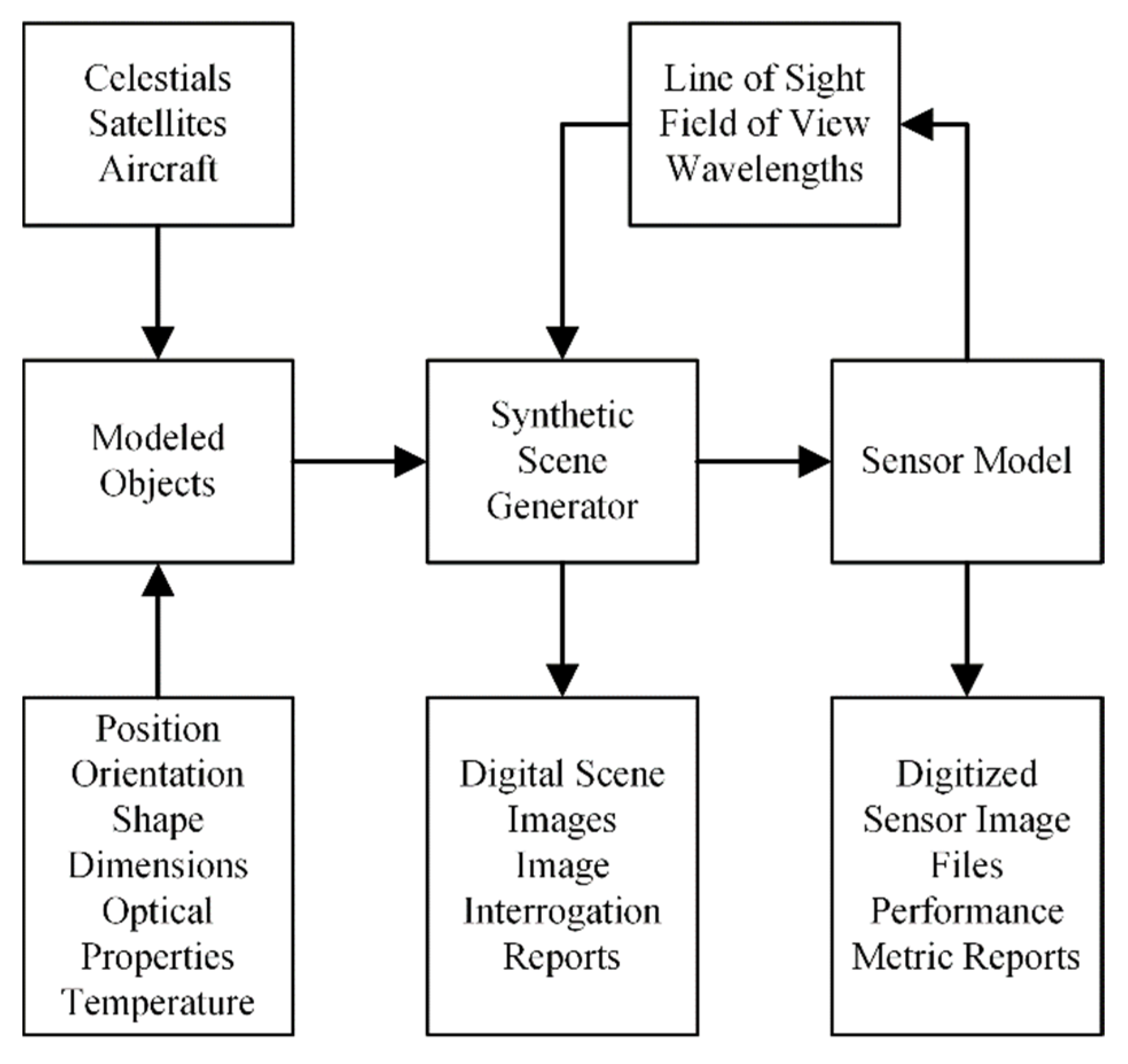
The EOIR module can simulate the detection, tracking, and imaging performance of electro-optical and infrared sensors for applications in Earth science and space situational awareness [33]. It supports the development, design, fielding, and operations of such systems. The module operates on a modeled Universe of Interest (MUI), which includes the Sun, the planets in the solar system, and stars. Users can design their own infrared objects and add them to it. Within the MUI, synthetic scene generator-sensor model pairs are placed and operated to produce images from various viewpoints or wavelength bands. The synthetic scene generator calculates radiation at the pupil entrance, while the sensor model adapts to spatial, spectral, optical, and radiometric aspects. In our system, we mainly used this module to obtain corresponding signal-to-noise ratio (SNR) data by customizing the infrared parameters of the target and sensor. The relationship between these components is shown in Figure 1.

Figure 1.
EOIR module overview.
2.2. COM Introduction
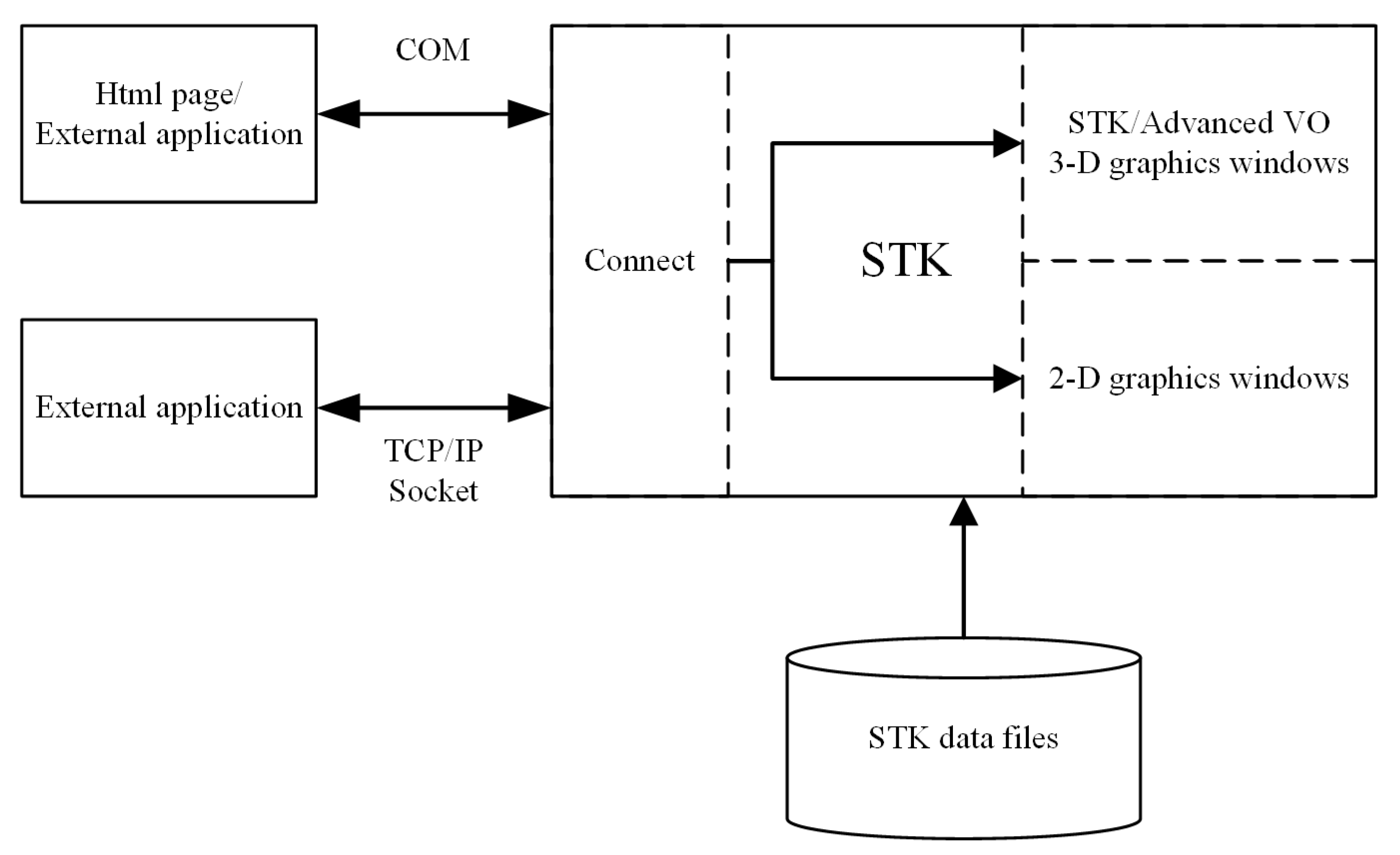
STK has two methods for secondary development: Connect mode and COM mode [34]. Figure 2 illustrates the operation of the two external interconnection methods of STK. Connect mode was originally designed to operate STK over TCP/IP by sending commands. Although the command design is characterized by readability, customizability, and platform independence, it has significant limitations such as supporting only built-in report graphs, manual parsing of returned data, and poorly designed error messages which make debugging difficult. COM’s purpose is to enable building custom solutions using STK. Additionally, it supports programming languages such as C#, Java, and C++, and provides the ability to control and automate STK objects, manage their lifecycle, and access data provider tools. This enables users to integrate STK scenes into their own systems, reducing the difficulty of developing visualization solutions. We took advantage of COM’s custom output to reduce the time overhead of interacting with STK. In addition, we temporarily switched to Connect mode to complete settings such as constellation parameters and target property data when COM did not have the corresponding methods.

Figure 2.
STK external interconnection diagram.
2.3. Function Design
The observation of point targets in the deep-space background by the EOIR module poses a challenge to the normal operation of the simulation scenario owing to the complex processing flow and high-resolution image output. Even at 64 × 64 resolution, the entire system can only generate 1 frame per second (FPS). For real-time target recognition algorithms, this is not enough to support their analysis of target micromotion. To balance accuracy and performance, we divided the process into two parts: target area and background area. The EOIR module simulates the high-confidence targets, while the stars and background are produced by an external system model based on a Central Processing Unit (CPU).
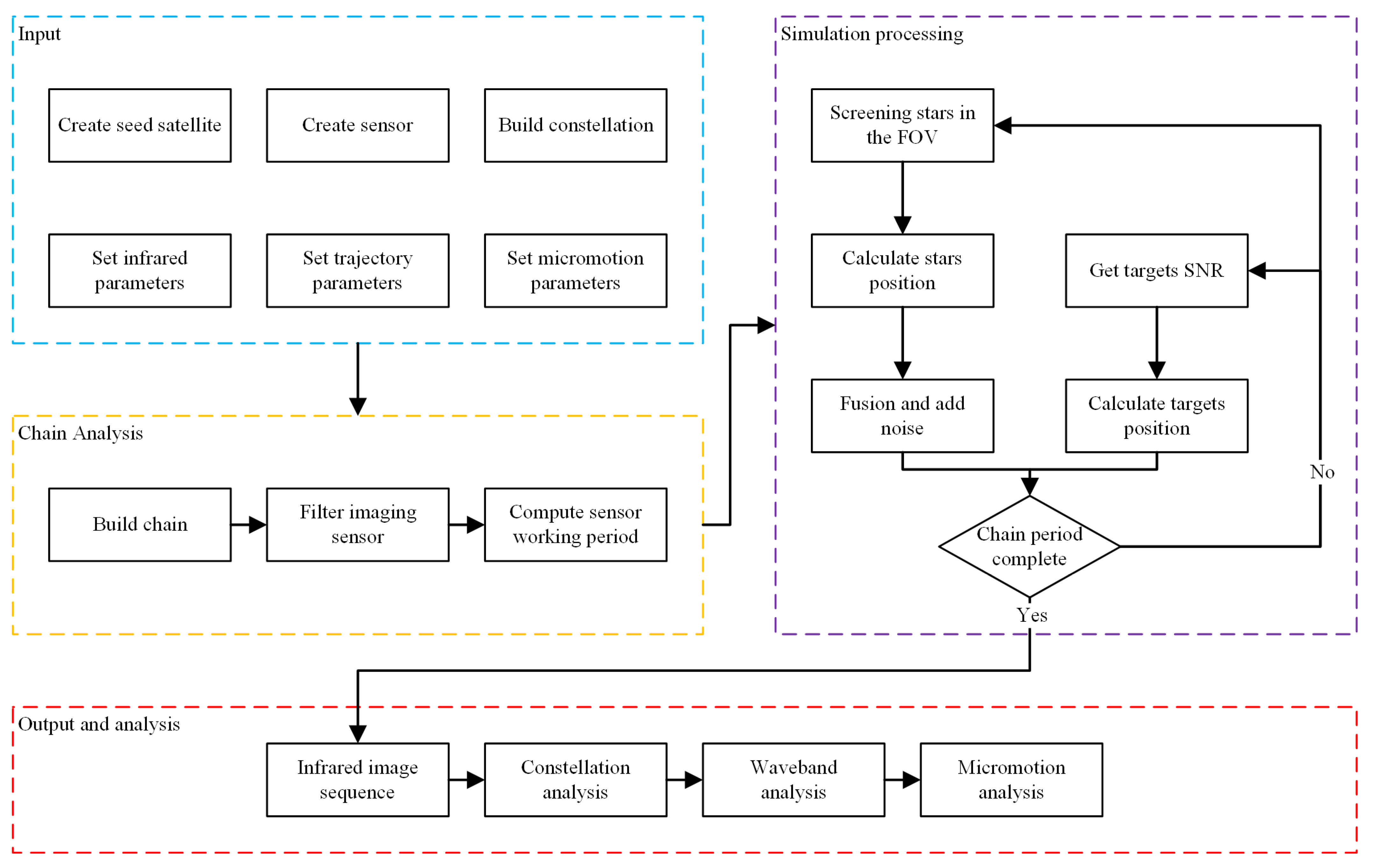
Figure 3 illustrates the functional flow of the system. Our fast simulation strategy addresses the performance challenge by improving the simulation process and optimizing the program execution, while optimizing the time complexity of the algorithms in the background generation to further enhance the simulation efficiency. At the onset of the simulation, we connected with STK [25] and established the target and seed satellite that carries the infrared sensor to complete the scenario initialization as input. Next, we generated the satellite constellation from the seed satellite, filtered the sensors involved in imaging through chain analysis, recorded their imaging periods, and removed other satellites from the scenario. During the simulation process, the target part contacts the STK data provider service to obtain the SNR of the sensor for each target in bulk. The background part first performs a preliminary screening of stars contained in the nearby table through sensor pointing and field of view (FOV), and then calculates their positions in parallel [18]. Finally, we merge the target and background and introduce diffraction effects and noise [35] asynchronously to complete the image simulation. After the imaging period ends, the system generates infrared image sequences and analyzes them in terms of constellation, waveband, and target micromotion.
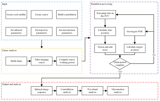
Figure 3.
System process.
3. Star Background Simulation
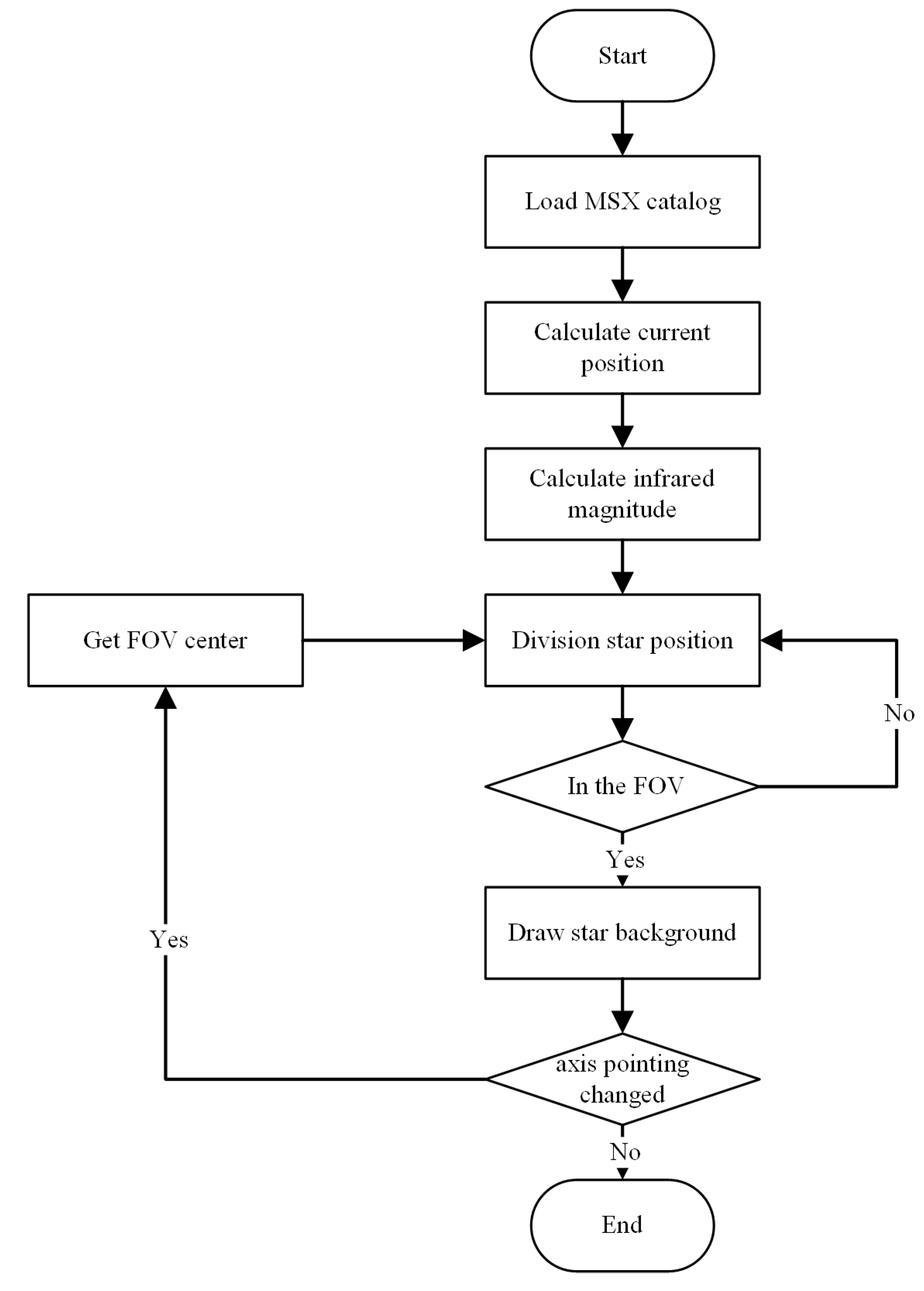
Given that the simulation scenario spans less than one day, the change in the position of stars relative to Earth can be considered negligible. Thus, the initial position of each star can be assumed to be static throughout the simulation. The process for simulating the star background is illustrated in Figure 4. Firstly, we read the data from the MSX catalog to obtain the initial position and the proper motion of the star. Next, we calculated both the right ascension and declination of the star at the beginning of the simulation, and the infrared magnitude of stars at different wavelengths. This information is stored in a database that adopts the format of latitude/longitude grid-latitude band, which enhances the efficiency of the background simulation module as it facilitates the search for stars in the FOV based on the optical axis point.

Figure 4.
Star background simulation process.
3.1. Star Catalog Selection
In practical applications, the background for space targets primarily consists of deep-space and various objects present in the universe. Given the limited FOV of sensors, we selected deep-space and stars as the background. Since the distance between stars and the Earth is vast, they can be considered as point targets in theory. The selection of a star catalog depends on the target’s equilibrium temperature and the sensor’s waveband range. In practice, the equilibrium temperature of the target is generally around 300 K, and the waveband range of the real sensor is generally medium wave or long wave. The MSX catalog provides spatial data, including the orientations and proper motions of 177,860 stars, as well as irradiance data ranging between 4 and 22 μm, making it a more suitable source of simulation data than other catalogs.
3.2. Infrared Magnitude Calculation
In the MSX catalog, the brightness of stars is represented by Jansky (Jy), which is denoted by [14].
where Jy is the unit of spectral flux density, W is the unit of power and m is the unit of length.
Irradiance within a specific wavelength band is denoted as and measured in W⋅cm−2⋅μm−1, and the conversion relation is [14]:
where c is the speed of light and its value is 3 × 10⁸ m/s; λ is the wavelength.
In astronomy, we commonly use equivalent magnitude to represent the brightness of celestial bodies. Therefore, we converted the brightness of stars to equivalent magnitude for storage and calculation [15]. Infrared magnitudes are established with reference to apparent magnitudes. The infrared magnitude of the requested star s1 is represented as m1. The irradiance of the zero-magnitude star and the star are represented as and , respectively. We can then express the relationship between these values using Equation (3):
By combing in Equations (2) and (3), it is possible to directly convert from the catalog Jy to the corresponding infrared magnitude. This conversion provides a straightforward method for determining the brightness of stars in infrared wavelengths:
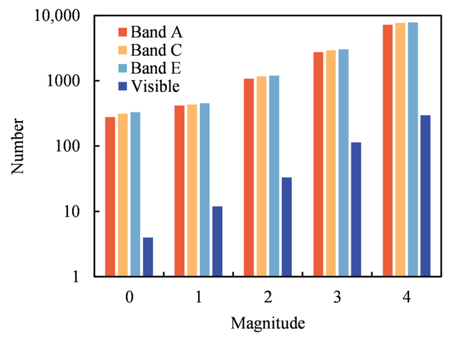
The relevant information from this catalog is presented in Table 1, including the number of stars with the same brightness in different infrared bands, as shown in Figure 5. Owing to the difference in the wavelength bands, there is a significant difference in the radiant fluxes corresponding to zero magnitude stars in band A and band C. However, the difference between band A and band C is not significant in terms of the number of stars of different magnitudes by calculation. Stars observed in the infrared band at each magnitude are one order of magnitude higher than those in visible light. Therefore, the influence of stars in the background should not be ignored.

Table 1.
The flux of zero-magnitude stars in MSX catalog.

Figure 5.
Number of stars of different band and magnitude in MSX catalog.
3.3. Lookup Table Design
The actual position of the star during the simulation time may not match the catalog owing to the motion of both the star and the Earth. Therefore, before the simulation starts, it is necessary to conduct spatial and temporal processing of the catalog. In our system, we mainly considered the effects of the proper motion of stars. Equation (5) calculates the right ascension and declination of the star at the beginning of the simulation in the J2000 coordinate system [18]:
where and are the right ascension and declination of the star at the simulation moment. The values and are the right ascension and declination recorded by the catalog. The values and denote annual proper motion of the right ascension and declination. This, , is the time difference between the simulation moment and the initial moment in years.
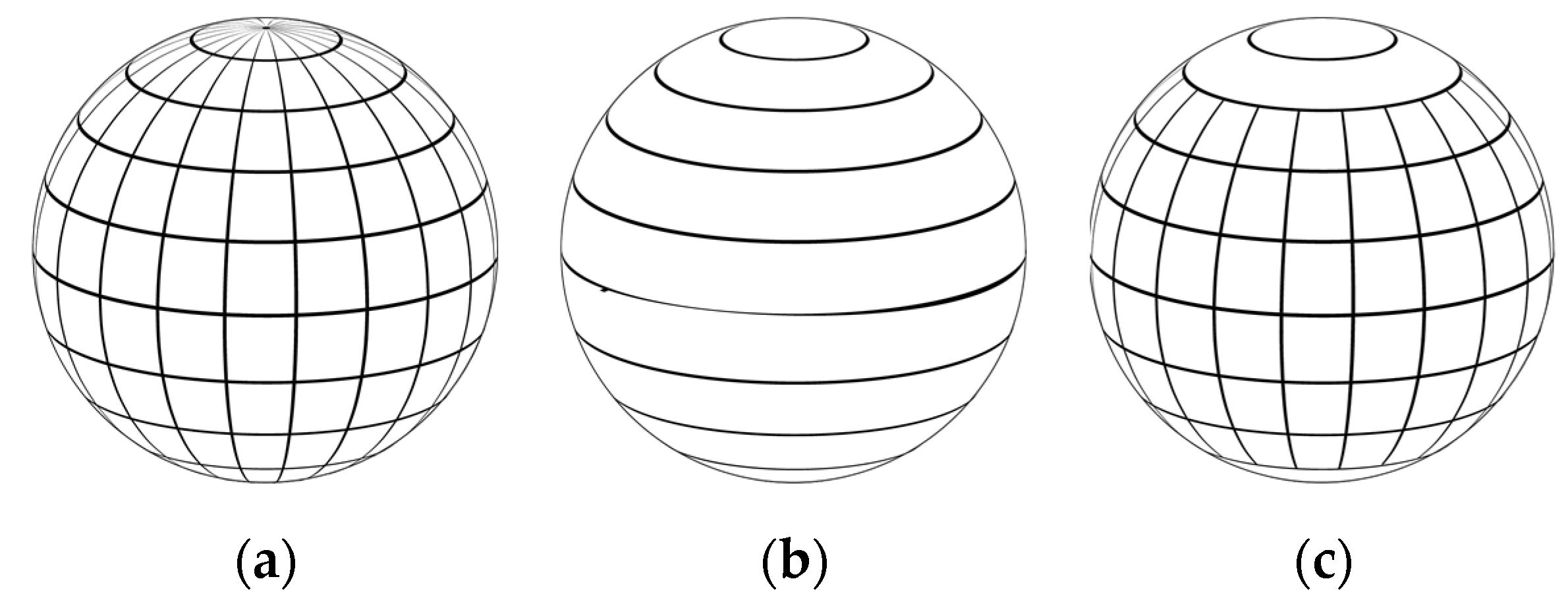
Additionally, the uneven distribution of stars in the catalog means that processing all the data in each frame would take excessive time. To address this issue, star sensors often use star map partitioning to accelerate the star detection process. For our database, we adopted a common partitioning method used in the field [36]. A longitude–latitude grid is used when the latitude along the optical axis is less than 60°, with one grid per degree; other high-latitude regions adopt a latitude band division with one band per degree of latitude. We created a two-dimensional array of size 360 × 180 to reduce the time complexity from O(n) to O(1) by space for time. This corresponding grid can be loaded based on the sensor’s optical axis point and FOV size; the required data can be obtained through deserialization, avoiding the traversal of the catalog during simulation. Because the array stores star data of high-latitude regions in the first grid corresponding to the latitude, it also avoided complex cross-region issues. The three catalog division methods are shown in Figure 6.
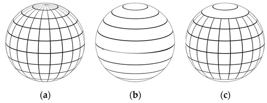
Figure 6.
Different partition methods: (a) Mash table; (b) Latitude table; (c) Comprehensive table.
3.4. Star Brightness Calculation
We calculated the stellar dynamic range using the specifications of the Space Infrared Imaging Telescope (SPIRIT III) sensor on the MSX satellite. This instrument underwent sufficient corrections before the measurement to ensure the accuracy of the results. Equation (6) shows the exact calculation, where the dynamic range of the star is determined by its own irradiance and the sensor noise equivalent irradiance (NEI) and saturated equivalent irradiance (SEI) together.
where and are the dynamic range and magnitude of the star, is the dynamic range of the sensor, and and are the irradiance of the 0-magnitude star and target star, respectively. For instance, in the case of the C band in the MSX catalog, stars with magnitudes less than 4 are not relevant and can be ignored during storage, which simplifies subsequent star filtering. The relevant information is presented in Table 2.
Table 2.
Dynamic range of infrared magnitude of MSX catalog.
The diffraction effect causes the star’s infrared radiation to be imaged as a point with a certain area as it passes through the optical system. To improve the accuracy of the simulation’s background, we considered the primary diffraction spot in the background simulation and assumed that the energy of the star obeys a Gaussian distribution in Equation (7) within the spot [37].
where are the coordinates of the target on the sensor, and is the standard deviation which indicates the width of the point diffusion.
The radius of the Airy spot is given by Equation (8). Combining the pixel pitch of the sensor, we can calculate the size of the Airy spot and the gray values of different pixels based on the dynamic range of the star.
where λ is the wavelength, L is the focal length, and D is the diameter of the optical pupil.
4. Simulation Experiments and Validation
4.1. Parameter Design
4.1.1. Walker Constellation Design
Walker constellations are based on the T/P/F for distributing the satellites in a constellation [38]. T is the total number of satellites in the constellation, P is the number of planes, and F is an interplane phasing designation. The right ascension of the ascending nodes (RAAN) and the mean anomaly of the jth satellites on the ith plane are described by Equations (9) and (10).
where S is the number of satellites per plane, Ω is the RAAN, and M is the mean anomaly. In the experiment, we built a Space Tracking and Surveillance System (STSS)-like Walker satellite constellation [39,40] with four satellite orbital planes and seven satellites in each plane. The main parameters of this constellation are presented in Table 3. The chain analysis reveals the participation of 10 satellites in the simulation scenario’s imaging process for the target. Given that the STK scenario imposes a constraint on the quantity of infrared sensors, extraneous satellites were eliminated before the simulation calculation.
Table 3.
Seed satellite and Walker constellation parameters.
4.1.2. Sensor Design
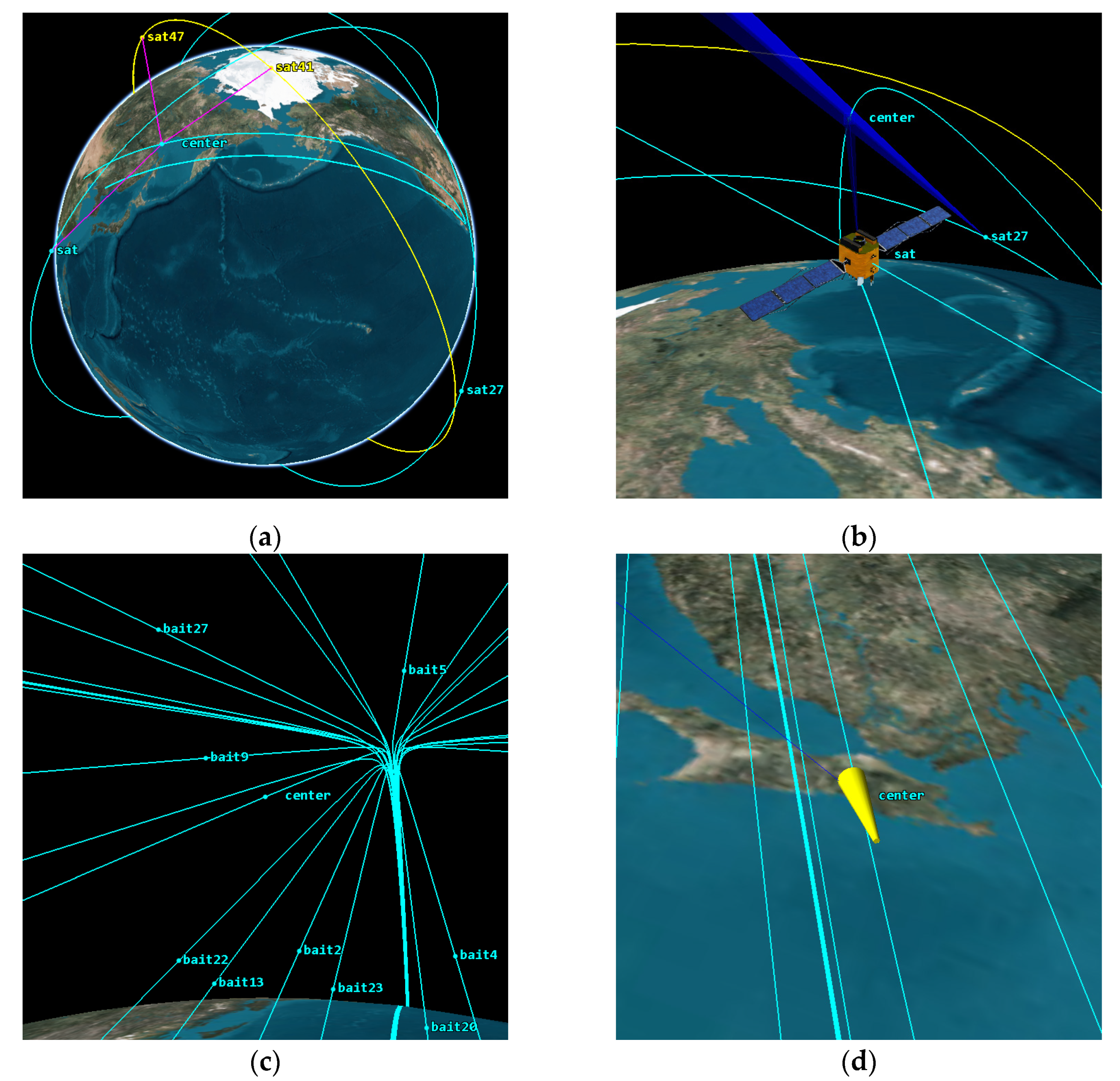
The sensor parameters were modeled after SPIRIT III. The main parameters of this sensor are divided into four aspects: spatial, spectral, optical, and radiometric. The spatial aspect sets the FOV and the number of pixels. The spectral aspect sets the number of intervals. The optical aspect sets the focal length and pupil diameter. The radiation aspect sets the NEI and SEI. To accurately simulate the target observation scenario and calculate the chain access durations, we imposed constraints on the distance and elevation angle. The specific parameters are detailed in Table 4. Figure 7a shows the overall situation of this simulation scenario and Figure 7b shows the scenario where three satellites in the Walker constellation observe the target group at the same time.
Table 4.
Sensor main parameters.

Figure 7.
Simulation scenario from multiple perspectives: (a) Full view; (b) Satellite view; (c) Group view; (d) Target view.
4.1.3. Target Design
Our observation object was a target group comprising one principal target named center and 29 secondary targets named bait. The trajectory parameters are outlined in Table 5. We assumed that the target trajectory was an arc that starts at 129.67° E, 40.86° N and ends at 118.40° W, 34.10° N after 1614 s. The ground distance of the trajectory was 9179 km, with a maximum altitude of 825.45 km. The complete trajectory of the target in the J2000 coordinate system was generated using the Runge–Kutta method. These methods incorporate random directions and sizes of tangential velocities to the position and velocity of the primary target at the release time. Figure 7c shows the scene of target group diffusion in this simulation scenario.
Table 5.
Targets trajectory parameters.
Each type of target has different parameters. In terms of shape, cone and sphere are generally considered to be the most common target types, and the cylinder is a container for placing targets. In terms of attitude, we assumed that cones type targets perform spin and precession, and sphere and cylinder type targets perform rolling [41]. In terms of temperature, we set the initial temperature of the target to 350 K and gradually reduced it to 328 K as the target moved [42,43,44]. Table 6 provides specific parameters for the above settings, and Figure 7d shows the shape of the main targets in the simulation scenario.
Table 6.
Targets infrared and attitude parameters.
4.2. Simulation Analysis
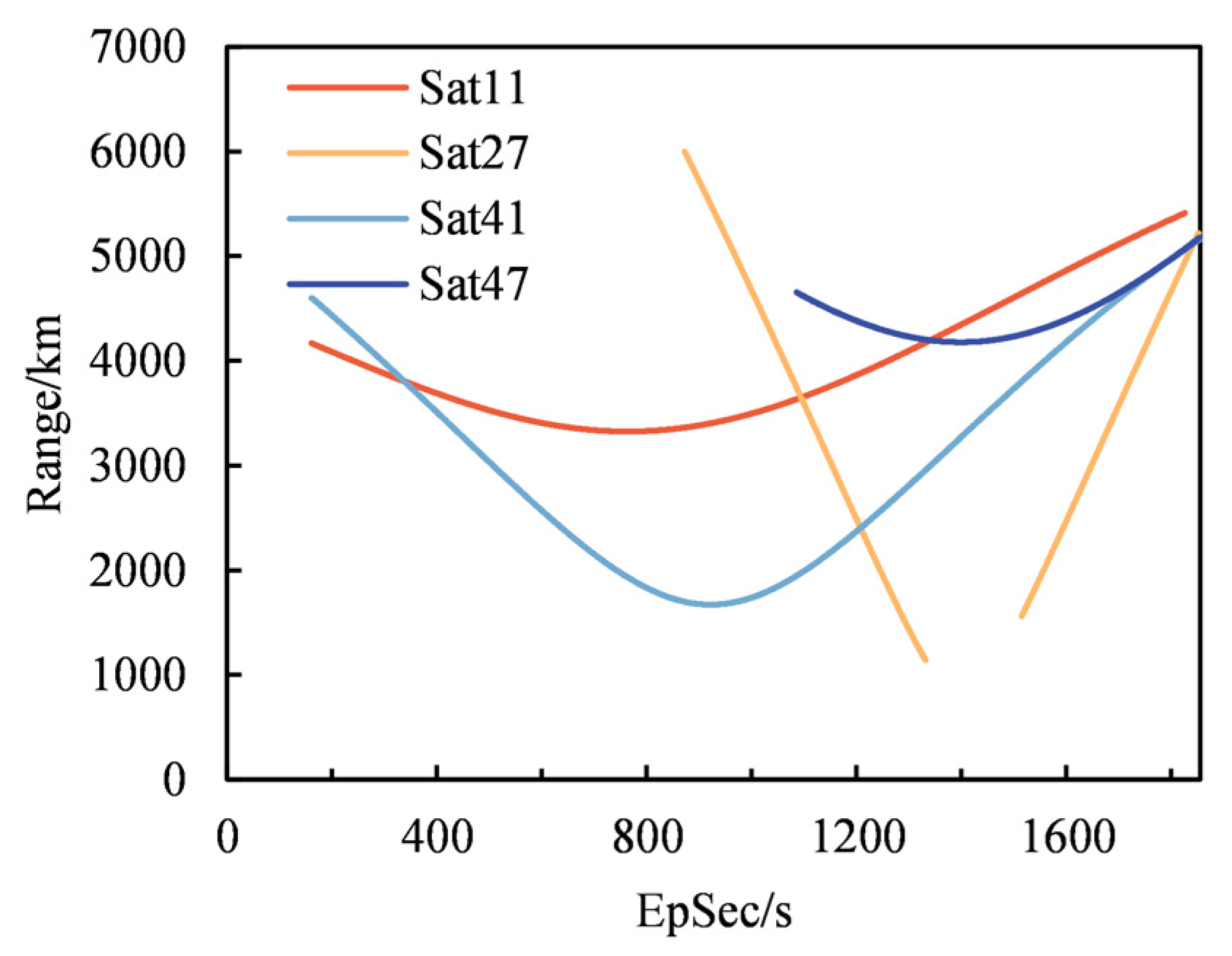
The position changes of the target group in the image plane are caused by several factors including the observation distance, direction of the optical axis, and relative motion between targets. We analyzed several satellites to describe the characteristics of the target group under different conditions. Sat11, located in the first orbital plane, has observed the trajectory throughout the entire journey, and the distance between the targets did not change significantly. Both Sat27 in the second orbital plane and Sat47 in the fourth orbital plane face the direction of target dispersion and provide different views of the target’s motion; this helps illustrate the motion more intuitively than the other satellites. Sat41 closely observed the target group from the side. Figure 8 shows the variation in distance from these satellites to the main target over time.
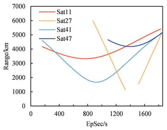
Figure 8.
Distance between satellites and the main target.
4.2.1. Constellation Analysis
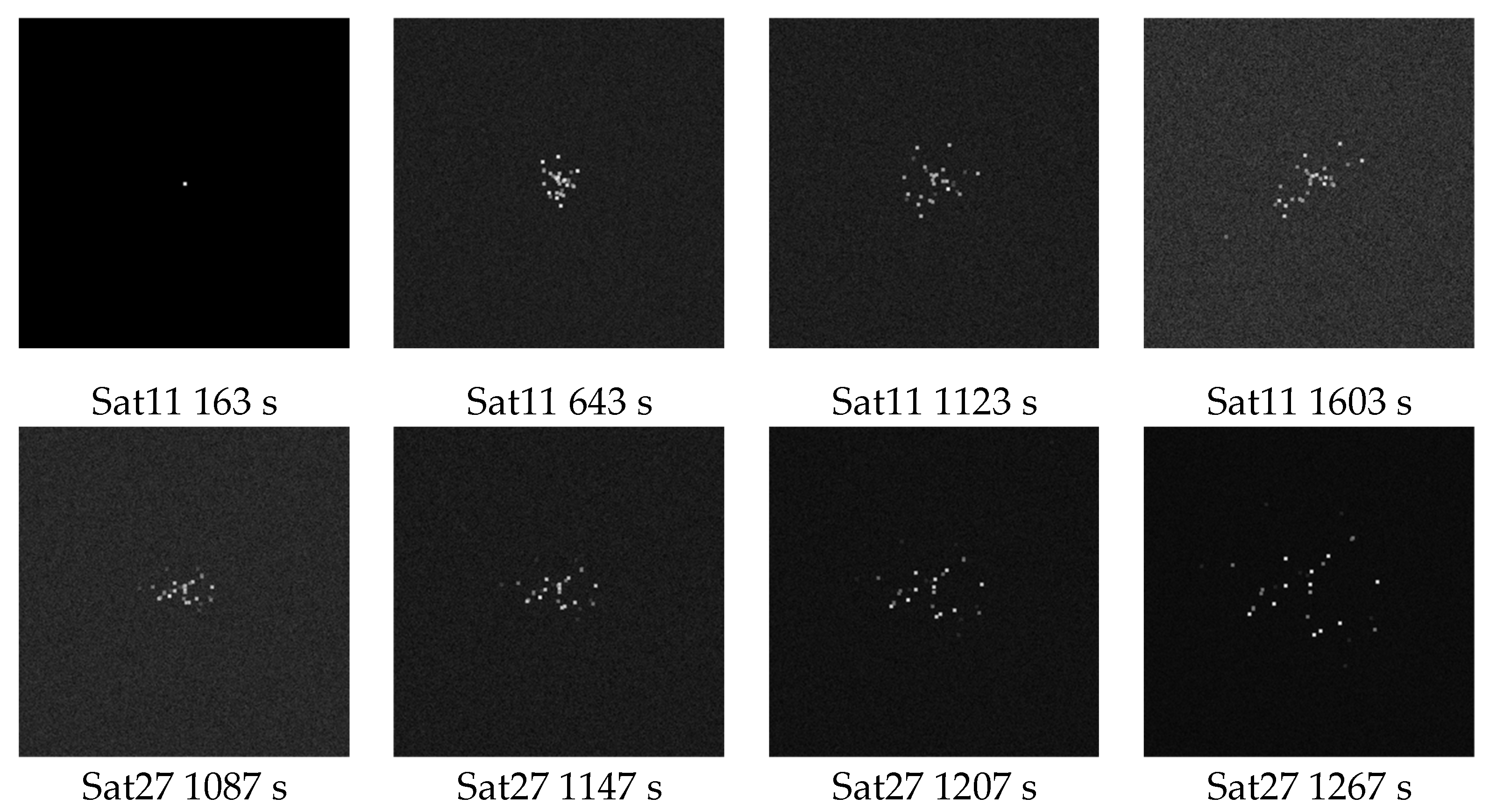
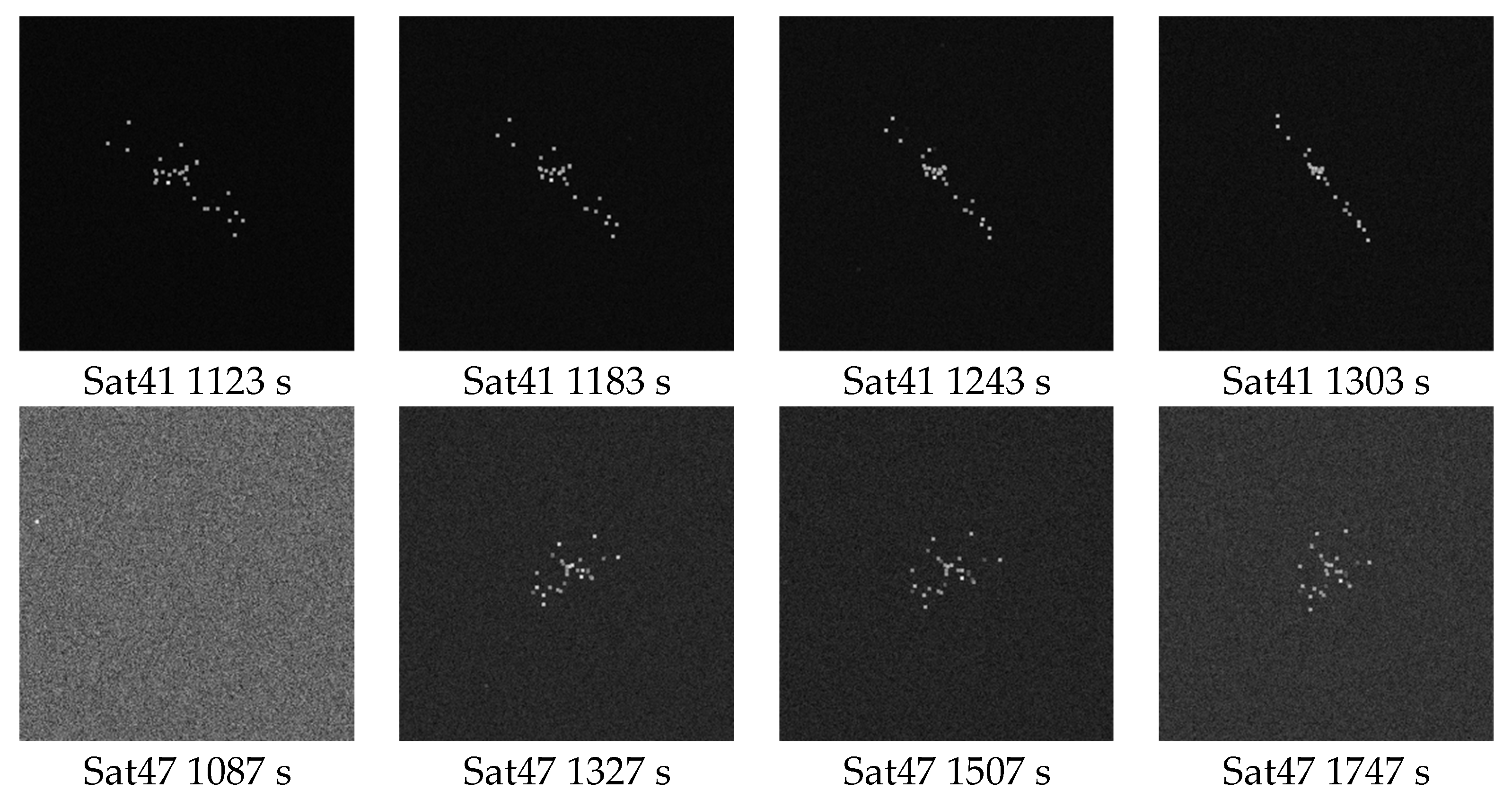
The results from sensor imaging are displayed in Figure 9. Upon analysis, the following characteristics were identified when the constellation imaged the targets:
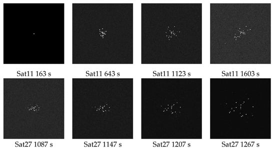

Figure 9.
Image results in band A from different satellites to targets.
Taking the image from Sat11 as an example, the target group was a bright spot at the beginning. As time progressed, each target consistently spread outward, and the images showed a general spreading trend. Because of the high-speed movement of both the satellites and targets, the relative angles between them underwent constant changes. For instance, images taken by Sat41 evolved from scattered to concentrated. With respect to observational efficacy, during the constellation imaging period, satellites (e.g., Sat27 and Sat47) that pass through the orbits plane of the target group have a lower probability of mutual occlusion during imaging which makes them suitable for the classification and tracking of target groups. In conclusion, observing from multiple perspectives using a constellation ensures that complete spatiotemporal distribution information of the target group is collected. Thus, it is essential to make targeted adjustments to the trajectory of potential observation targets when designing a satellite constellation to enhance the constellation’s tracking ability.
4.2.2. Waveband Analysis
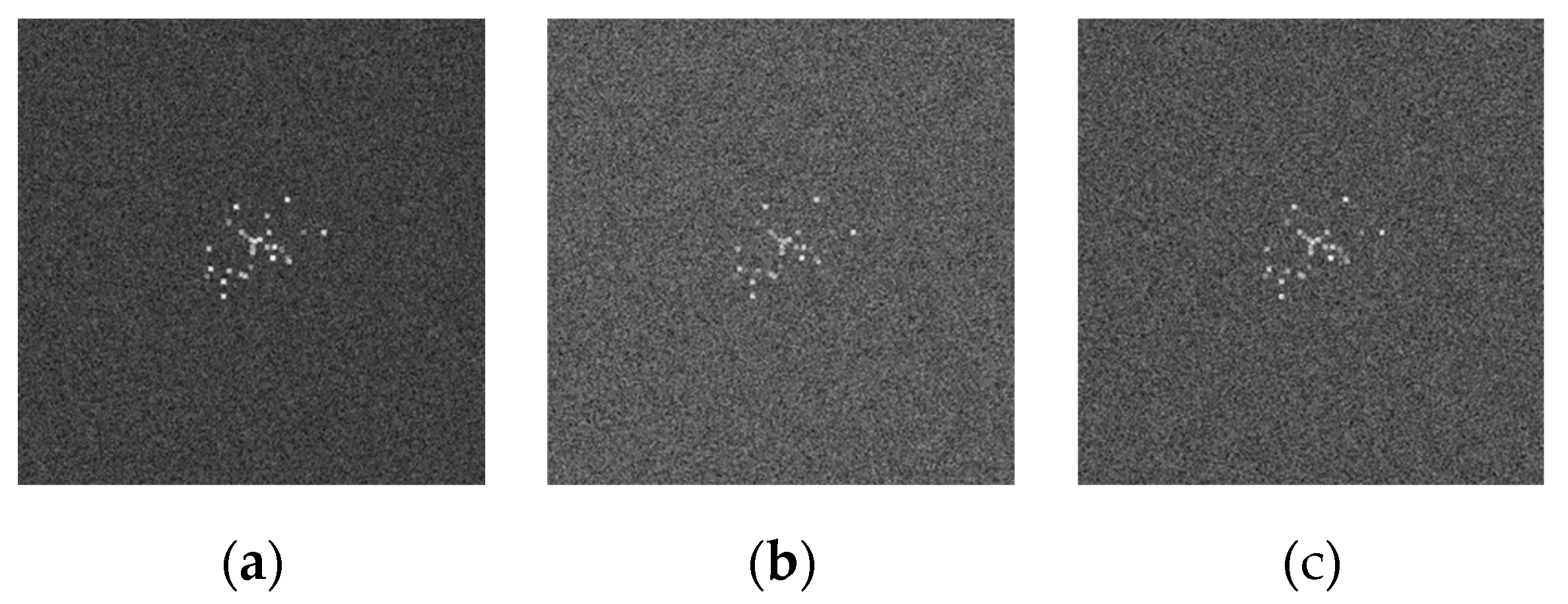
Targets’ different infrared properties and distance from the sensor cause them to show different levels of brightness on the sensor at the same time. Because of changes in the solar vector and observation distance, some of a target’s signal may be lost in the sensor system noise response, rendering it undetectable. Additionally, certain targets have a lower signal than stars in the FOV, making them harder to identify within the image. Figure 10 displays the imaging results of satellite Sat11 sensors on a target group simultaneously using different wavebands. The simulation scenario indicates that, because of the exclusion of interference from the imaging time of the sensor and the spatial relationship between the sensor and targets, the targets exhibit the same geometric features; the SNR of the medium wave sensor is more significant than that of the medium-long wave and long wave sensors. Traversing the sensor band reveals that increasing the band’s width can significantly enhance the sensor’s SNR within the background noise of deep space.
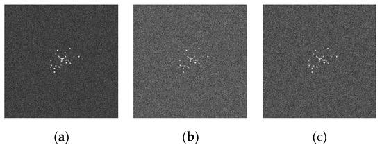
Figure 10.
Images in different bands from Sat11 to targets: (a) Band A; (b) Band C; (c) Band E.
4.2.3. Micromotion Analysis
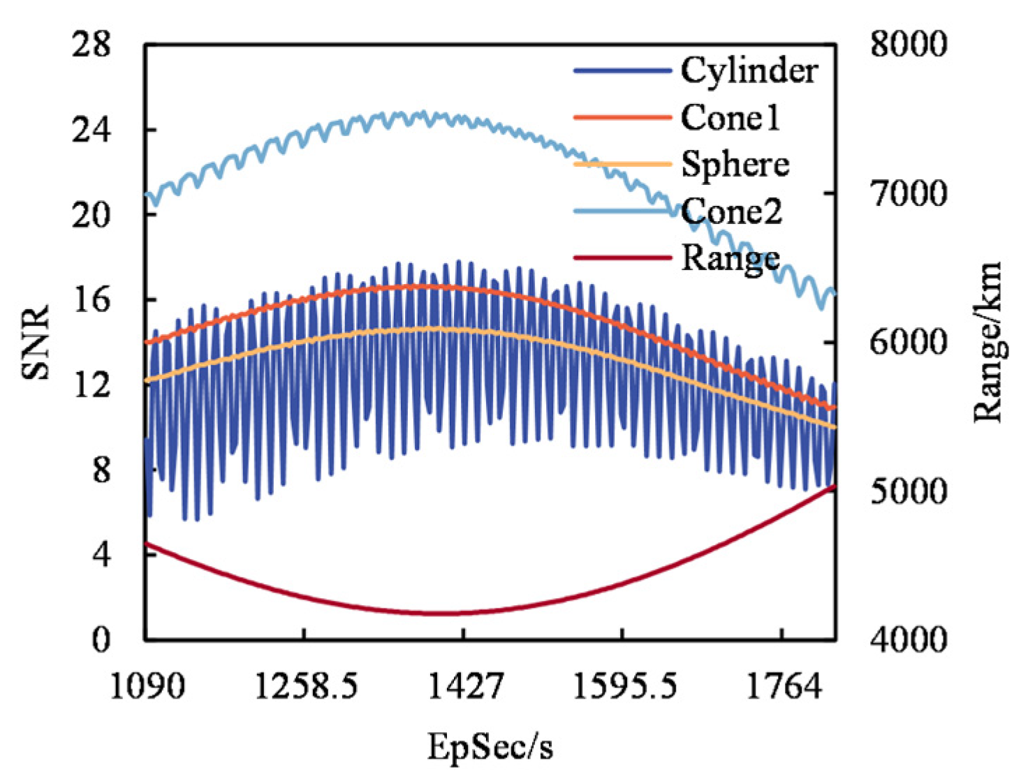
Target micromotion causing a change in projected area is an important factor contributing to the variability of target SNR. The proposed method supported the analysis of the micromotion characteristics in shorter time steps by enhancing the performance of the simulation system. A representative of each target type was selected for analysis; their corresponding SNR values over time are presented in Figure 11, obtained from the Sat47 sensor. Under the present circumstances, the Cylinder, which has notable variations in projected area across multiple dimensions, experiences a considerably greater change in SNR because of micromotion compared to other targets over the entire observation period. The observation effect of micromotion varies greatly at different time periods owing to changes in the sensor’s viewpoint during long-term observation. The Cone2 target exhibits the smallest fluctuation during the period closest to the sensor. Figure 12 displays the effect of short-term target micromotion after excluding the interference caused by sensor line-of-sight changes. Cylinder rolling causes a more pronounced change in projected area than other types of targets, whereas Sphere rolling has the least effect on the change in projected area and the weakest SNR fluctuations. The different reflectivity of two cone-shaped targets with the same size leads to differences in average SNR. Cone2, with higher precession angle and frequency, exhibits significant differences in terms of the amplitude and frequency of SNR changes. Our system, combined with STK, can differentiate between the various micromotion modes of space targets with different shapes. Establishing a practical micromotion model of complex targets can be a crucial means of distinguishing target types in practical scenarios.

Figure 11.
Sat47 observes SNR changes for various types of targets.
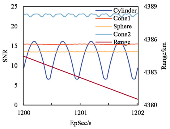
Figure 12.
Effect of targets micromotion on SNR.
4.2.4. Speed Analysis
Since STK did not provide specific implementation details, we compared the original method mainly in terms of simulation time cost. We used the parallel implementation for the computation of the positions and gray values of the stars and targets. Although the time complexity was kept as O(n), the engineering goal of saving time in the simulation phase was achieved. Meanwhile, we used C#’s asynchronous approach to allow the simulation system to perform subsequent computations, and also implemented noise templates to pre-generate noisy data in scenarios requiring higher output performance, further reducing the time cost. We evaluated the performance of the simulation system under different satellite constellations and sensor parameters using the Monte Carlo method; Table 7 shows the rate of simulated image generation at different resolutions. Our system demonstrated a remarkable 186-fold improvement in CPU-based simulation of the output of MSX satellite sensors for target imaging when compared to STK. This satisfied the observation of targets by 20 sensors in the satellite constellation at the same moment, surpassing the number of target-visible satellites in the above case of an STSS-like constellation. Despite a decline in the frame rate of the system after the resolution increase, it maintained 32 FPS at a resolution of 1 K × 1 K, fulfilling the real-time simulation requirement. This advancement significantly enhances the usability of STK in infrared simulation and improves the viewing experience. In the future, we will continue to optimize the simulation process and use GPU-based methods to refine the simulation requirements at high resolutions.
Table 7.
System simulation performance at different resolutions.
5. Results and Discussion
The improvements of proposed method compared to others are shown in Table 8. In terms of simulation performance, while the original techniques excelled in establishing simplistic space-based infrared simulation scenarios and presenting results in an intuitive manner [7,29], they encountered challenges when confronted with complex scenarios. Furthermore, they lacked support for fast infrared simulation output. Conversely, the proposed method achieved real-time simulation of space-based sensors on space point targets, thereby enhancing its practicality. In terms of background generation, the original STK-based methods could generate star backgrounds without requiring complex setups [7]. However, the absence of customization options for star catalogs and the inability to export star simulation results limited their practicality. Other star background simulation methods accurately calculated star positions [17,18], yet they did not provide further discussion of spatial targets within the FOV. In this regard, the proposed method generated high-quality star background for the targets, effectively compensating for STK’s deficiency in star simulation. In terms of target features, the original techniques primarily focused on the influence of target attitude while setting the temperature to a fixed value or a linear function of time [7,37,41,43]. In contrast, the proposed method embraced a dynamic temperature model and accounted for the impact of micromotion during the simulation process. In terms of development mode, the original methods fulfilled their specific application requirements through secondary development of STK, leveraging its data analysis capabilities [20,21,22,23], but they did not mention the program maintainability and expandability. The proposed method employed contemporary tools and connection modes to enhance the system’s scalability. In short, we established the foundation of a modern space-based simulation platform.
Table 8.
Overview of the improvement of the proposed methods.
6. Conclusions
This paper presents a background model, including star motion and infrared brightness, based on the MSX catalog. We have achieved autonomous and controllable deep-space background creation from external catalog data. The visual simulation system can obtain infrared information in the deep-space background of space-based scenes and generate image sequences of point target groups. Compared with the default EOIR process, our approach supports 20 sensors simultaneously observing the target groups and achieved simulation of 30 FPS on 1 K × 1 K high-resolution sensors. It therefore supports the rapid construction of complex space-based scenarios and provides efficient high-quality data support for target identification and tracking algorithms.
Author Contributions
All the authors contributed to this study. Conceptualization, C.G. and P.R.; Investigation, C.G. and Y.L.; Methodology, P.R. and Y.L.; Software, C.G.; Data curation, C.G.; Funding acquisition, P.R.; Project administration, P.R. and Y.L.; Supervision, Y.L.; writing—original draft preparation, C.G.; writing—review and editing, P.R. and Y.L. All authors have read and agreed to the published version of the manuscript.
Funding
This research was funded by Innovation Project of Shanghai Institute of Technical Physics of the Chinese Academy of Sciences, grant number CX-375.
Institutional Review Board Statement
Not applicable.
Informed Consent Statement
Not applicable.
Conflicts of Interest
The authors declare no conflict of interest.
References
- Gartley, M.G. Polarimetric Modeling of Remotely Sensed Scenes in the Thermal Infrared. Ph.D. Thesis, Chester F. Carlson Center for Imaging Science, Henrietta, NY, USA, 2007. [Google Scholar]
- Latger, J.; Cathala, T.; Douchin, N.; Goff, A.L. Simulation of active and passive infrared images using the SE-WORKBENCH. In Proceedings of the Defense & Security Symposium, Orlando, FL, USA, 9–13 April 2007. [Google Scholar]
- Murrer, R.; Thompson, R.A.; Coker, C.F. Recent Technology Developments for the Kinetic Kill Vehicle Hardware-In-The-Loop Simulator (KHILS); Air Force Research Laboratory: Wright-Patterson Air Force Base, OH, USA, 1998. [Google Scholar]
- Nelsson, C.; Hermansson, P.; Nyberg, S.; Persson, A.; Persson, R.; Sjökvist, S.; Winzell, T.J. Optical signature modeling at FOI. In Proceedings of the Optics/Photonics in Security and Defence, Stockholm, Sweden, 11–14 September 2006. [Google Scholar]
- Savage, J.; Coker, C.; Edwards, D.; Thai, B.; Kim, C.J. Irma 5.1 multi-sensor signature prediction model-art. no. 62390C. In Proceedings of the Optics/Photonics in Security and Defence, Orlando, FL, USA, 17–21 April 2006. [Google Scholar]
- Vaitekunas, D.A.; Holst, G.C.; Ramaswamy, S. Validation of ShipIR (v3.2): Methodology and results. In Proceedings of the Optics/Photonics in Security and Defence, Baltimore, MD, USA, 20–24 April 2006. [Google Scholar]
- Dai, H.; Zhang, Y.; Zhou, H.; Zhao, S. Infrared imaging simulation of midcourse ballistic target based on STK/EOIR. Electron. Opt. Control 2018, 25, 1–5. [Google Scholar]
- Helou, G.; Walker, D.W. Infrared Astronomical Satellite (IRAS) Catalogs and Atlases. Volume 7: The Small Scale Structure Catalog. In Proceedings of the Infrared Astronomical Satellite (IRAS) Catalogs and Atlases, USA, 1 January 1988; Volume 7, pp. 1–265. [Google Scholar]
- Egan, M.P.; Price, S.D. The MSX Infrared Astometric Catalog. Astron. J. 1996, 112, 2862. [Google Scholar] [CrossRef]
- Cutri, R.; Skrutskie, M.; Van Dyk, S.; Beichman, C.; Carpenter, J.; Chester, T.; Cambresy, L.; Evans, T.; Fowler, J.; Gizis, J. VizieR online data catalog: 2MASS all-sky catalog of point sources (Cutri+ 2003). VizieR Online Data Cat. 2003, II/246. [Google Scholar]
- Ishihara, D.; Onaka, T.; Kataza, H.; Salama, A.; Alfageme, C.; Cassatella, A.; Cox, N.; Garcia-Lario, P.; Stephenson, C.; Cohen, M. The AKARI/IRC mid-infrared all-sky survey. Astron. Astrophys. 2010, 514, A1. [Google Scholar] [CrossRef]
- Cutri, R.M.; Wright, E.L.; Conrow, T.; Bauer, J.; Benford, D.; Brandenburg, H.; Dailey, J.; Eisenhardt, P.R.M.; Evans, T.; Fajardo-Acosta, S.; et al. Explanatory Supplement to the WISE Preliminary Data Release Products. Explan. Suppl. WISE All-Sky Data Release Prod. 2011, 1. [Google Scholar]
- Hernán-Caballero, A.; Alonso-Herrero, A.; Hatziminaoglou, E.; Spoon, H.W.; Almeida, C.R.; Santos, T.D.; Hönig, S.F.; González-Martín, O.; Esquej, P. Resolving the active galactic nucleus and host emission in the mid-infrared using a model-independent spectral decomposition. Astrophys. J. 2015, 803, 109. [Google Scholar] [CrossRef]
- Huang, C.; Wang, J.; Gao, X.; Li, J. Application of infrared star catalog in ground-based infrared radiation measurement system. Infrared Laser Eng. 2013, 42, 2901–2906. [Google Scholar]
- Wang, Y.; Sun, X.; Zhang, H.; Chen, F. A new approach for extrapolating star flux using cross-matching multiple catalogues. J. Infrared Millim. Waves 2019, 38, 473–478. [Google Scholar]
- Miao, Y.; Wang, Z.; Wang, C.; Liu, S.; Peng, Q. Modeling and simulation of celestial background. J. Syst. Simul. 2005, 17, 267–269. [Google Scholar]
- Li, X.; Dong, Y.; Wang, Y.; Wang, J. Study of radiation of sky background model. Infrared Laser Eng. 2007, 90, 382–384. [Google Scholar]
- Hong, Y.; Xu, X. IR radiation scene generation model of celestial point source background. Mod. Def. Technol. 2011, 39, 170–175+182. [Google Scholar]
- Zhang, R.; Xu, S.; Chen, Z. Multi-target Flight Scene Simulation Based on STK/X. In Proceedings of the 2nd IEEE Advanced Information Technology, Electronic and Automation Control Conference (IAEAC), Chongqing, China, 25–26 March 2017; pp. 1139–1143. [Google Scholar]
- Li, L.; Wang, P. Research and application of visualization simulation system based on VC/STK. Comput. Digit. Eng. 2018, 46, 94–97+107. [Google Scholar]
- Huo, L.; Liu, Z.; Chen, L.; Zhao, W.; Qian, S. Design and implementation of STK remote control system based on C# Connect connection. Ship Electron. Eng. 2017, 37, 102–105. [Google Scholar]
- Zhang, Z.; Liao, X.; Gao, Y. Space orbit quick interception module design and simulation based on HLA and STK. J. Syst. Simul. 2013, 25, 2390–2396. [Google Scholar] [CrossRef]
- Zhang, Y.; Guo, Y.; Hong, J. Analysis of distributed inter-satellite link network coverage based on STK and Matlab. IOP Conf. Ser. Mater. Sci. Eng. 2019, 563, 052003. [Google Scholar]
- Guo, X.; Xi, C.; Pan, Z. Application of STK software in digital target scene simulation. Mod. Radar 2018, 40, 71–76. [Google Scholar] [CrossRef]
- Chen, Z.; Meng, Y.; Mao, J. Design and implementation of spatial situation simulation system based on STK. In Proceedings of the International Conference on Space Information Technology 2009, Beijing, China, 26–27 November 2010. [Google Scholar]
- Zhou, H.; Li, Z.; Li, X. Study of lnfrared Radiation Characteristics of Midcourse Ballistic Targets Based on STK/EOIR. Infrared 2017, 38, 21–25+48. [Google Scholar]
- Cao, C.; Wu, W.; Wang, Y. Detection of Space Target in and out of Field of View for Continuous Image Frame. In Proceedings of the Applied Optics and Photonics China (AOPC) Conference—Optical Spectroscopy and Imaging and Biomedical Optics, Beijing, China, 30 November–2 December 2020. [Google Scholar]
- Clark, R.; Fu, Y.; Dave, S.; Lee, R. Simulation of RSO Images for Space Situation Awareness (SSA) Using Parallel Processing. Sensors 2021, 21, 7868. [Google Scholar] [CrossRef]
- Wei, R.; Song, A.; Duan, H.; Pei, H. An Effective Procedure to Build Space Object Datasets Based on STK. Aerospace 2023, 10, 258. [Google Scholar] [CrossRef]
- Wang, F.; Liu, X.; Jiang, B.; Zhuo, H.; Chen, W.; Chen, Y.; Li, X. Low-loading Pt nanoparticles combined with the atomically dispersed FeN4 sites supported by FeSA-N-C for improved activity and stability towards oxygen reduction reaction/hydrogen evolution reaction in acid and alkaline media. J. Colloid Interface Sci. 2023, 635, 514–523. [Google Scholar] [CrossRef]
- Li, Q.; Zhao, D.; Yin, J.; Zhou, X.; Li, Y.; Chi, P.; Han, Y.; Ansari, U.; Cheng, Y. Sediment Instability Caused by Gas Production from Hydrate-bearing Sediment in Northern South China Sea by Horizontal Wellbore: Evolution and Mechanism. Nat. Resour. Res. 2023, 32, 1595–1620. [Google Scholar] [CrossRef]
- Li, Q.; Zhang, C.; Yang, Y.; Ansari, U.; Han, Y.; Li, X.; Cheng, Y. Preliminary experimental investigation on long-term fracture conductivity for evaluating the feasibility and efficiency of fracturing operation in offshore hydrate-bearing sediments. Ocean Eng. 2023, 281, 114949. [Google Scholar] [CrossRef]
- STK Help. Available online: https://help.agi.com/stk/#eoir/eoir_properties.htm?Highlight=eoir (accessed on 30 July 2023).
- Getting Started with Connect. Available online: https://help.agi.com/stkdevkit/index.htm#stkObjects/ObjModProgramming.htm?Highlight=COM (accessed on 30 July 2023).
- Zhang, Z. Research on Realistic Imaging of Space Scenes in Visible and Infrared Wavebands. Master’s Thesis, Zhejiang University, Zhejiang, China, 2004. [Google Scholar]
- Zhang, W. Research on Camera On-Orbit Radial Calibration and Ground Verification Methods Based on Infrared Catalog Extrapolation. Master’s Thesis, Shanghai Institution of Technical Physics Chinese Academy of Sciences, Beijing, China, 2017. [Google Scholar]
- Mao, H.; Li, X.; Wang, Z.; Su, Y.; Wu, K.; Ma, J.; Zhao, K. Simulation of infrared radiation from outer space targets and environment, and its generation technique of scene. Infrared Laser Eng. 2007, 36, 607–610. [Google Scholar]
- Guan, M.; Xu, T.; Gao, F.; Nie, W.; Yang, H. Optimal Walker Constellation Design of LEO-Based Global Navigation and Augmentation System. Remote Sens. 2020, 12, 1845. [Google Scholar] [CrossRef]
- Yu, E.; Xu, X. Study on the Method of STSS Space Coverage Performance. Comput. Simul. 2010, 27, 103–106. [Google Scholar]
- Mao, Y.; Zhang, D.; Wang, L. Simulation Analysis of Ballistic Missile Detection by STSS. Infrared Technol. 2015, 37, 218–223. [Google Scholar]
- Zhang, H.; Rao, P.; Xia, H.; Weng, D.; Li, Y. Modeling and analysis of infrared radiation dynamic characteristics for space micromotion target recognition. Infrared Phys. Technol. 2021, 116, 103795. [Google Scholar] [CrossRef]
- Zhu, D.; Shen, W.; Cai, G.; Ke, W. Numerical simulation and experimental study of factors influencing the optical characteristics of a spatial target. Appl. Therm. Eng. 2013, 50, 749–762. [Google Scholar] [CrossRef]
- Yuan, H.; Wang, X.; Zhang, K.; Ren, D.; Li, K. Analysis of the detection ability of midcourse ballistic targets in the complex environment. Infrared Laser Eng. 2019, 48, 302–311. [Google Scholar]
- Zhang, S. Simulation Study of Airborne Infrared Early Warning Imaging Target Trajectory Test. Master’s Thesis, Xidian University, Xidian, China, 2022. [Google Scholar]

Disclaimer/Publisher’s Note: The statements, opinions and data contained in all publications are solely those of the individual author(s) and contributor(s) and not of MDPI and/or the editor(s). MDPI and/or the editor(s) disclaim responsibility for any injury to people or property resulting from any ideas, methods, instructions or products referred to in the content. |
© 2023 by the authors. Licensee MDPI, Basel, Switzerland. This article is an open access article distributed under the terms and conditions of the Creative Commons Attribution (CC BY) license (https://creativecommons.org/licenses/by/4.0/).