Abstract
Road detection technology is an important part of the automatic driving environment perception system. With the development of technology, the situations that automatic driving needs to consider will become broader and more complex. This paper contributes a lightweight convolutional neural network model, incorporating novel convolution and parallel pooling modules, an improved network activation function, and comprehensive training and verification with multiple datasets. The proposed model achieves high accuracy in detecting drivable areas in complex autonomous driving situations while significantly improving real-time performance. In addition, we collect data in the field and create small datasets as reference datasets for testing algorithms. This paper designs relevant experimental scenarios based on the datasets and experimental platforms and conducts simulations and real-world vehicle experiments to verify the effectiveness and stability of the algorithm models and technical solutions. The method achieves an MIoU of 90.19 and a single batch time of 340 ms with a batch size of 8, which substantially reduces the runtime relative to a typical deep network structure like ResNet50.
1. Introduction
Road detection is an important yet challenging task in driverless technology. It is a crucial component of the visual navigation system for autonomous vehicles. Currently, deep-learning-based road detection algorithms are widely used for autonomous driving. These algorithms employ fully convolutional neural networks (CNNs) to extract features and classify image regions or pixels [1,2,3]. This enables the extraction of more abstract features and high detection accuracy. With the application of deep learning in image semantic segmentation, road detection methods using deep neural networks and segmentation [4,5] architectures emerge. This propels progress in road detection. However, such networks focus on semantic segmentation accuracy over real-time performance. Given hardware constraints in vehicles, lightweight real-time algorithm models are essential for various driving tasks in autonomous scenarios.
On the basis of the road structure characteristics of the current autonomous driving scenarios mainly studied, the road structure can be roughly divided into structured roads and unstructured roads. Structured roads usually have road markings and clear boundaries, with flat and less or no defects on the road surface, while unstructured roads typically do not have clear lane lines or road edges, and the road surface may be uneven or the road composition elements may be complex and varied. At this stage, the research technology for structured road detection under normal weather and light conditions is relatively well established. However, in reality, weather conditions and lighting conditions are not always constant, and road conditions are not always well-structured, so it is difficult for autonomous driving systems based on structured roads to cope with the demands of further development of their research, and the algorithms need to be strengthened to detect and recognize the complex environment of unstructured roads. There are two main problems with the current unstructured path:
- (1)
- The boundary between the drivable area and the non-drivable area of the unstructured road may be blurred. The road edge is irregular and discontinuous, and there is no clear lane line. Its complexity has a great influence on the accurate extraction of the edge points, which poses a challenge to the traditional edge fitting method.
- (2)
- The structured road has fewer obstacles, while the unstructured road environment has more complex road conditions and often has various kinds of interference, which may appear at random locations, vehicles, people or animals, and non-motorized vehicles suddenly appear behind buildings, with higher environmental variability, requiring real-time detection of interference information and differentiation from the feasible driving area.
Considering the accuracy and real-time performance of the feasible region detection of the model, as well as the value of unstructured road research in civil, commercial, and military fields, this paper aims at the drivable area detection of unstructured roads for autonomous driving. Based on the characteristics of unstructured roads and the theory of neural networks and deep learning, a lightweight convolutional neural network model for the identification of drivable areas in complex situations of autonomous driving is established.
2. Background
The method based on deep learning is based on the traditional neural network. It mainly extracts features through convolutional neural networks (CNNs) and classifies the pixels in the image area. It can extract more abstract image features. Through the training of a large amount of datasets, the model parameters are iteratively optimized, which can achieve higher road detection accuracy. However, due to the large processing data, higher requirements are placed on the computing hardware.
The AlexNet network [6] improves the local response normalization (LRN) layer of the generalization ability of the model, expands the data through data augmentation, and modifies the network structure to achieve random dropout to prevent the model from overfitting. Alvarez [7] et al. proposed to extract image features through CNN, combined with texture description factors to detect road driving areas in real time. Long [8] et al. from the University of California, Berkeley, proposed the idea of fully convolutional networks (FCNs), which extends the original CNN structure and decomposes the semantic segmentation task into a combination of encoder and decoder for the first time. Mendes et al. [9] proposed a road detection algorithm based on a fully convolutional neural network, which transforms the road detection problem into a two-class image semantic segmentation problem and introduces image context information, which has excellent performance on the KITTI road detection dataset and once achieved a road detection performance ahead of other algorithms. PSPNet [10] and Deeplab [3] use a spatial pyramid model to combine multi-scale contextual information, while Bilinski [11], Yang [12], and Li [13] et al. use dense layers at the decoder side to inject the advantage of multi-level feature reuse, and Jiqing C [14] et al. propose a recurrent GAN-based image enhancement network (IEC-Net) to enhance diverse features of the input image. Some of the recent studies have used attentional mechanisms to capture richer global contextual information [15,16,17,18,19,20,21,22,23,24,25,26,27,28,29,30]. YOLACT [4], D3NET [5], and CycleGAN [14] network structures are proposed for the detection of drivable areas and to achieve good results. Although the effectiveness of these approaches has been validated on datasets collected from structured environments (e.g., Cityscapes [31] and ADE20K [32]), their effectiveness in unstructured and complex environments (e.g., rural, wilderness, and harsh weather) has not been verified.
In terms of enhancing the lightweight of semantic segmentation algorithms, many lightweight models have been proposed, such as MobileNetV1, MobileNetV2 [33,34], ESP-Net [35], Enet [36], LAANet [37], and CCC [38]; also, Shuhao Ma [39] performed real-time image semantic segmentation by improving the DeepLabV2 network model, which obtains real-time operation by significantly reducing the computational and parametric quantities in the network model, but at the same time, it also reduces the measurement accuracy.
To summarize, there is currently a lack of neural network research that balances accuracy and real-time performance for the detection of drivable areas in complex unstructured environments.
3. Method
In the field of computer vision, road detection can be categorized as a semantic segmentation task, where classification is performed at the pixel level. For the detection of drivable areas, this is a binary classification problem. Differentiated features learned across various stages are projected onto the pixel space to generate the segmentation output, which can then be visualized as needed.
This paper realizes pixel-level classification and global area detection. It distinguishes drivable areas from non-drivable ones under complex road conditions and changing weather. The model needs to be lightweight for deployment on embedded platforms. Model depth, calculation amount, and precision are constrained to account for hardware variability and uncertainty in real-world use.
3.1. Structural Model
The lightweight deep learning network model constructed for traveling area identification is shown in Figure 1. A to H, in turn, through multiple convolution models implement changes to the dimension of the input image and feature extraction operation, generating preliminary image feature mapping, and then through the parallel pooling module I + J operations implement multi-scale hierarchical image feature extraction and scale. Different levels of features map the input feature fusion layer K for operation, and the fused features are reduced in dimension through the convolution layers L and M. The feature mapping dimension is reduced to the dimension of the detection target type. Finally, the up-sampling is carried out in the network layer N to restore the image scale, and the prediction results are obtained. In the later part of the article, the network training process, input and output data will be visualized.
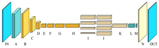
Figure 1.
Network model structure diagram.
In Table 1, the input data are of the form (CH, H, W), which denote the number of channels, height, and dimension, respectively. The column of the kernel parameter indicates the parameter factor of the first convolutional kernel or the parameter factor of the pooling kernel of the first convolutional operation within the corresponding layer in the row. The constant coefficients of the kernel parameters in the form of multiplication indicate the number of repetitions of the convolution operation in the corresponding layer in that row, where the first convolution operation completes the channel number transformation, feature extraction, and dimensionality enhancement operations. The repetition operation after the first convolution does not change the channel number of the corresponding input and output, indicating the inverse residual module operation. The step size column indicates the step size parameter selected for the convolution or pooling operation, where each row in the column vector form indicates the step size used for the convolution operation of the corresponding order.

Table 1.
Overall network structure.
3.2. Convolution Module
In the initial network design, convolutional layers were constructed to separate each input channel, with multiple small kernels convolving the data channel-wise. However, depthwise convolution alone is insufficient to expand the feature space for subsequent operations [40,41,42]. Therefore, a high-dimensional point convolution kernel of size 1*1 is introduced after the depthwise convolution, and the multiple mapping features after the depthwise convolution are fused and transformed into high-dimensional mapping features, while the relationship between the mapping features of each channel is established, which finally forms the convolution calculation process as shown in Figure 2.
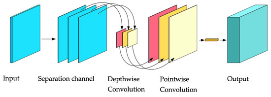
Figure 2.
Convolution calculation process diagram.
This method reduces the number of parameter factors compared to the direct use of high-dimensional large convolutional kernels, thus reducing the amount of operations. However, due to the decreasing number of parameter factors, the fitting ability of individual network layers also decreases relatively, and the network needs to be built by combining methods such as classical convolutional layers and deepening network layers to get good output. Therefore, the lightweight optimization of the residual module is combined with the residual module of ResNet and MobileNetV2. Therefore, combining the residual module of ResNet and MobileNetV2’s lightweight optimization of the residual module [34], the full convolutional layer is first used to increase the data dimensionality, and then different convolutional steps and inflated convolutional architectures are used to construct the inverted residual layer to complete the depthwise convolution and dimensionality change operations. The internal structure of the inverted residual layer is shown in Figure 3. Firstly, the channel number of feature mapping is increased by a 1*1 convolution kernel. Then, the convolution operation is carried out by a 3*3 convolution kernel. Subsequently, the channel number of feature mapping is either returned to the initial state or transformed to other dimensions using a 1*1 convolution kernel; combined with residuals, and finally, the output is completed.
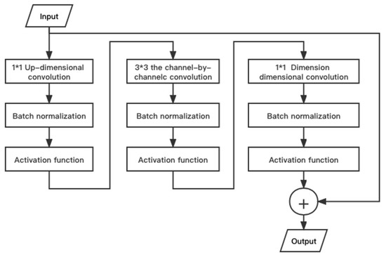
Figure 3.
Inverted residual layer structure diagram.
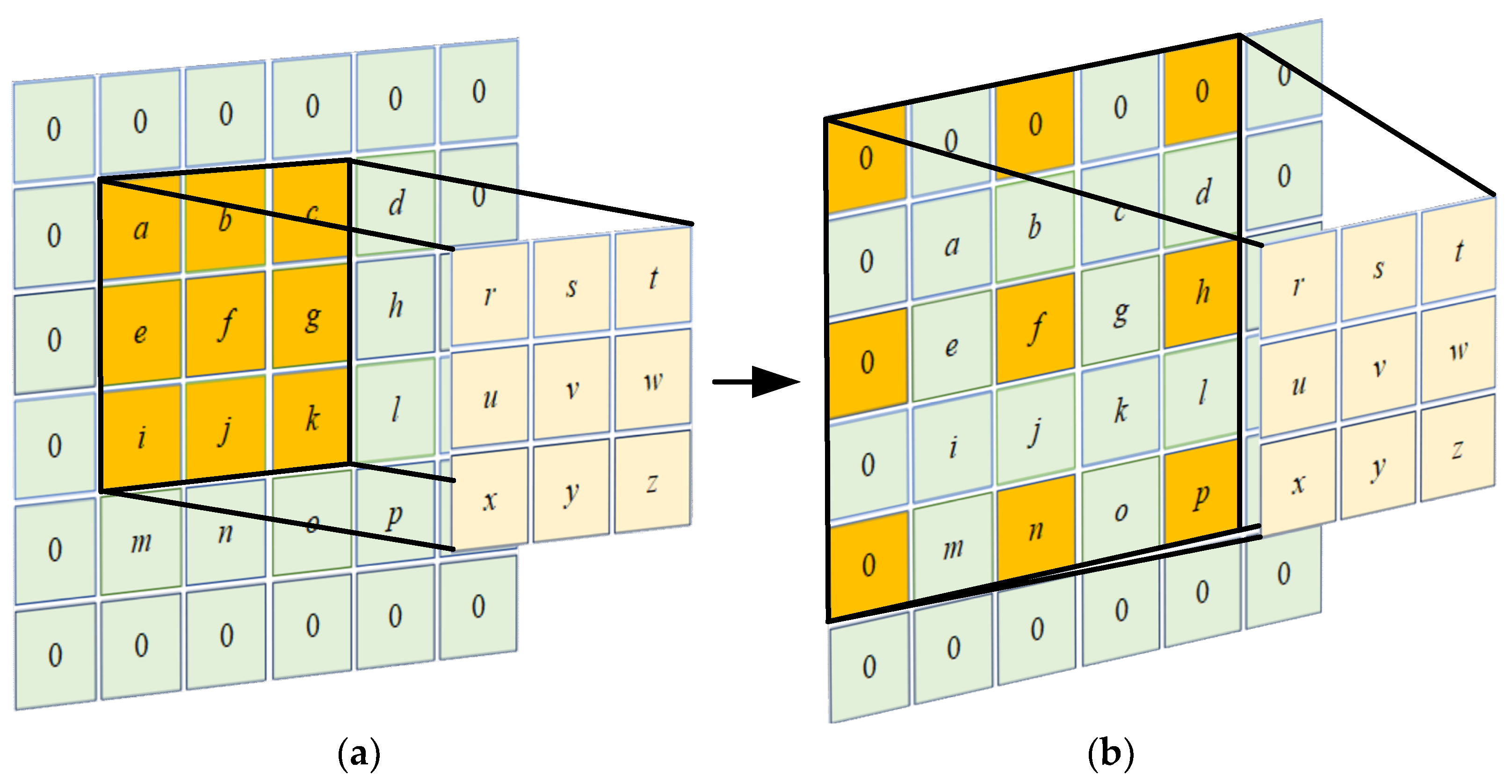
In the inverted residual layers G and H, the theory of dilated convolution [43] is introduced, which transforms depthwise convolution into depthwise dilated convolution. The convolution kernel of the dilated convolution is the same as the ordinary convolution; that is, the parameters are the same, but the area on the original image corresponding to the convolution kernel is changed, and the distance between the adjacent elements extracted by the convolution kernel is enlarged by the expansion coefficient. As shown in Figure 4b, with other parameters unchanged, the dilated convolution with an expansion coefficient of 2 expands the region by one week compared to the ordinary convolution, and the sensory field becomes twice the original, which facilitates the integration of context information, while the mapping feature resolution does not change. The expansion coefficient of the inverted residual layers G and H is 2.
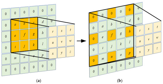
Figure 4.
Comparison between dilated convolution and ordinary convolution: (a) ordinary convolution area and (b) dilated convolution region with an expansion coefficient of 2.
3.3. Parallel Pooling Module
Based on the idea of multi-process and multi-thread parallelization in computer systems and along with the theory of spatial pyramid pooling, this paper designs a parallel pooling module as shown in Figure 5.
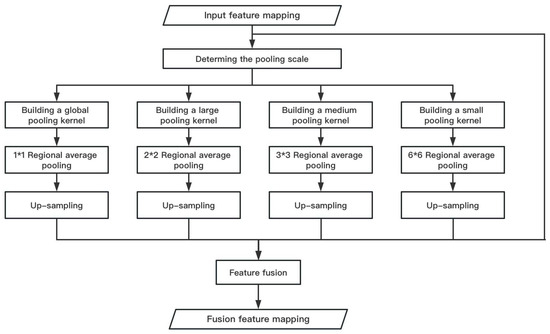
Figure 5.
Parallel pooling module calculation process diagram.
The parallel pooling modules can be divided into parallel pooling layer I and parallel up-sampling layer J. The parallel pooling layer is pooled by four pooling channels of different scales. Each channel automatically adjusts the parameter values of the pooling kernel and stride through internal calculation based on the size of the input feature mapping. The input feature mapping is divided into 1*1, 2*2, 3*3, and 6*6 target areas, and then, the average pooling processing is performed on each area. According to the size of the area, a variety of pooling scales including global average pooling and pooling kernels of different sizes are realized, and then, the pooled feature maps are scaled to the same size through parallel up-sampling operation, entering the next feature mapping fusion stage.
In the feature mapping fusion stage, since the research content of this paper is a binary classification problem, there are a few types of image features to be considered, and the feature mapping similarity of the network model near the output end is high. Therefore, the feature fusion layer K uses the summation method for feature fusion. At the same time, in order to make better use of the global information and spatial position relationship, the feature mapping used in the feature fusion operation includes not only the four feature mappings output by the parallel pooling module but also the feature mapping before pooling, that is, the feature mapping output by the inverted residual layer H.
The parallel pooling module broadens the network structure and enhances the nonlinearity of the network without deepening the network depth too much. Compared with the decoder network of linear superposition network layer, it simplifies the number of network layers and the amount of calculation. At the same time, it can aggregate the feature maps of different regions at different scales and obtain more global information.
3.4. Activation Function and Loss Function
Combining parametric ReLU with ReLU6, this paper proposes an activation function PRLU6 based on improved ReLU. The greatest advantage of PReLU is that it enhances its robustness when using low-precision calculations [44]. The equation can be formalized as follows:
Among them, α is the parameter factor, and the initial value is set to 0.01 with reference to leaky ReLU [45]. The update and optimization of α can be realized with backpropagation during network training. When x ≥ 0, the activation function is similar to ReLU6, which can ensure that the activation function value is within a certain range when the data value is too large and avoid the calculation loss when the model is applied on the low-precision platform.
In the shallow network structure from network layer A to network layer F, the activation function adopts PRLU6, which reduces the amount of calculation and retains the network characteristics better than ReLU. While in the deep network, the cost of applying the nonlinear activation function will decrease, resulting in an improved performance of Hard Swish. Compared with PRLU6, it can better handle parallel pooling modules. Therefore, in the network layer G to L, the network module uses Hard Swish. The functional expression is given in Equation (2).
4. Dataset
The following four datasets are constructed and used in the following experiments.
- (1)
- The global drivable area dataset includes 8000 instances of the BDD100k [46] dataset and 16,063 instances of the IDD dataset [47]. The road, parking, and ground annotations in the BDD100k dataset and the road, parking, and drivable fallback annotations in the IDD dataset are used as the target drivable areas, and the corresponding conversion masks are generated. The scene includes scenes of multiple pedestrians, vehicles, and obstacles in cities and villages, as well as lane-less roads, paved roads, and unpaved roads.
- (2)
- The road drivable area dataset contains 80,000 copies of BDD100k dataset data and corresponding conversion masks. This dataset mask file is mainly generated based on the area/drivable kinds and area/alternative kinds in the annotation of the BDD100k dataset, which can be used as a control group of unstructured environments to verify the applicability of the model structure of this paper in a variety of road situations.
- (3)
- The off-road environment drivable dataset, containing 7436 data from the RUGD dataset [48], and the corresponding transformation masks validate the generalizability of the model in this paper in the face of somewhat challenging data situations.
- (4)
- Self-built small datasets are used to simply evaluate the applicability of this paper’s model in the Chinese environment and also participate in the training and testing of this paper’s network model together with the validation and test sets in the above (1) and (2) datasets.
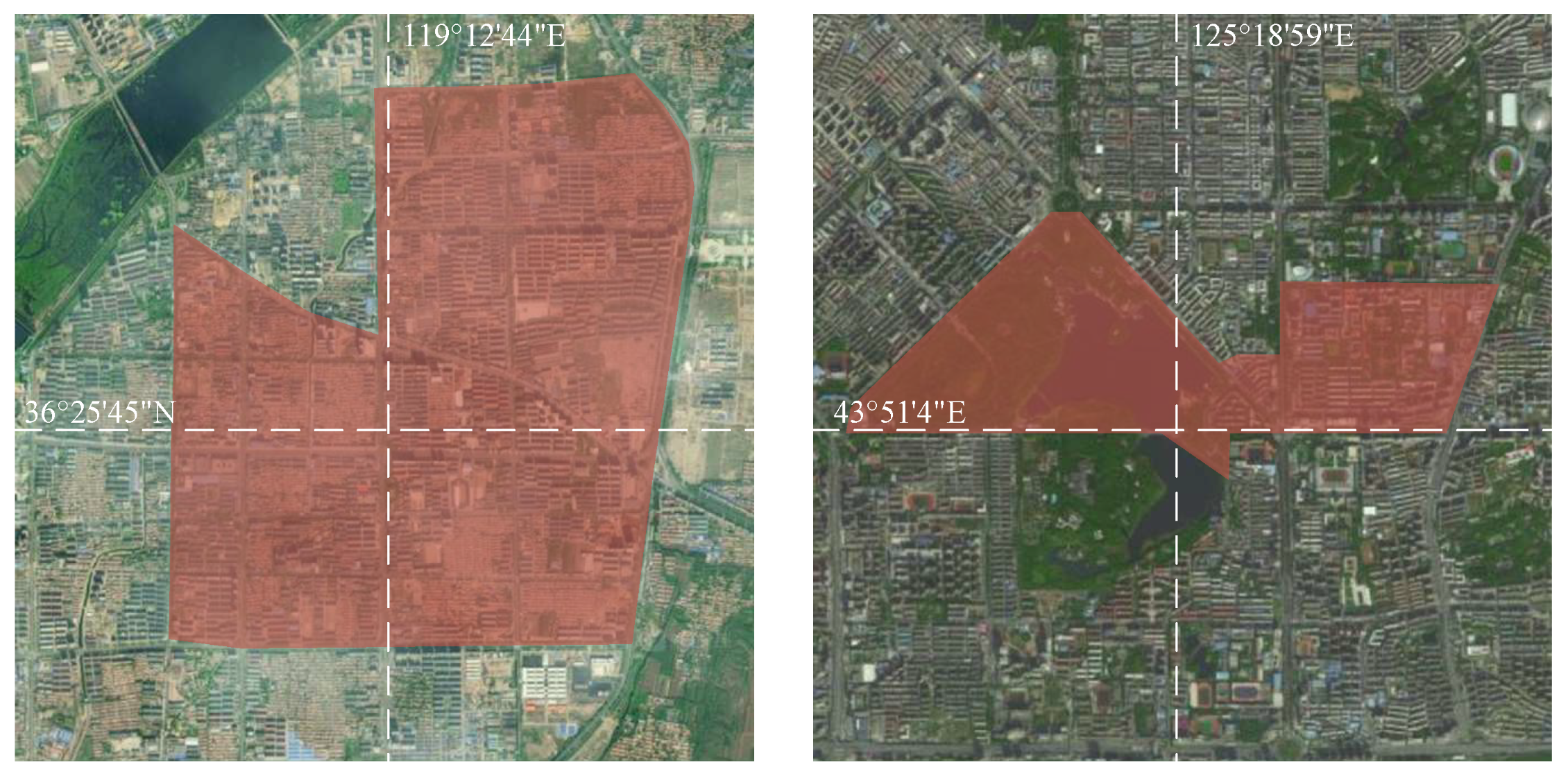
Since most public datasets consist of scenes from other countries that are unrepresentative of Chinese environments, we collected information and data using industrial cameras, smart handheld devices, and other equipment across various regions in China. The data cover diverse conditions including residential areas, campus roads, urban–rural junctions, day and night, clear and inclement weather, and different times of day and seasons. The data format includes continuous videos and individual single-frame pictures, covering old lane-free, unmarked highways, community unstructured roads, rural dirt roads, night unmarked highways, rain and snow-covered roads, etc. At the same time, network data collection is carried out to supplement the self-collected data set. Part of the acquisition range is shown in Changchun, China, in Figure 6. Compared with the publicly available dataset, the dataset collected in this paper has some quantitative gaps. Sample self-picked datasets are shown in Figure 7. Therefore, this paper randomly selects some images in the self-built dataset for annotation.

Figure 6.
Partial data collection scope.
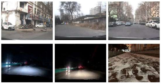
Figure 7.
Sample images from self-selected datasets.
5. Results
The algorithm used in this paper is built and tested on Windows 10 and Ubuntu 20.04 LTS platforms, using the dataset constructed in our previous work. The hardware includes an Nvidia GTX 1660Ti GPU, 16GB DDR4 memory, and an AMD Ryzen 5800H 3.20 GHz CPU.
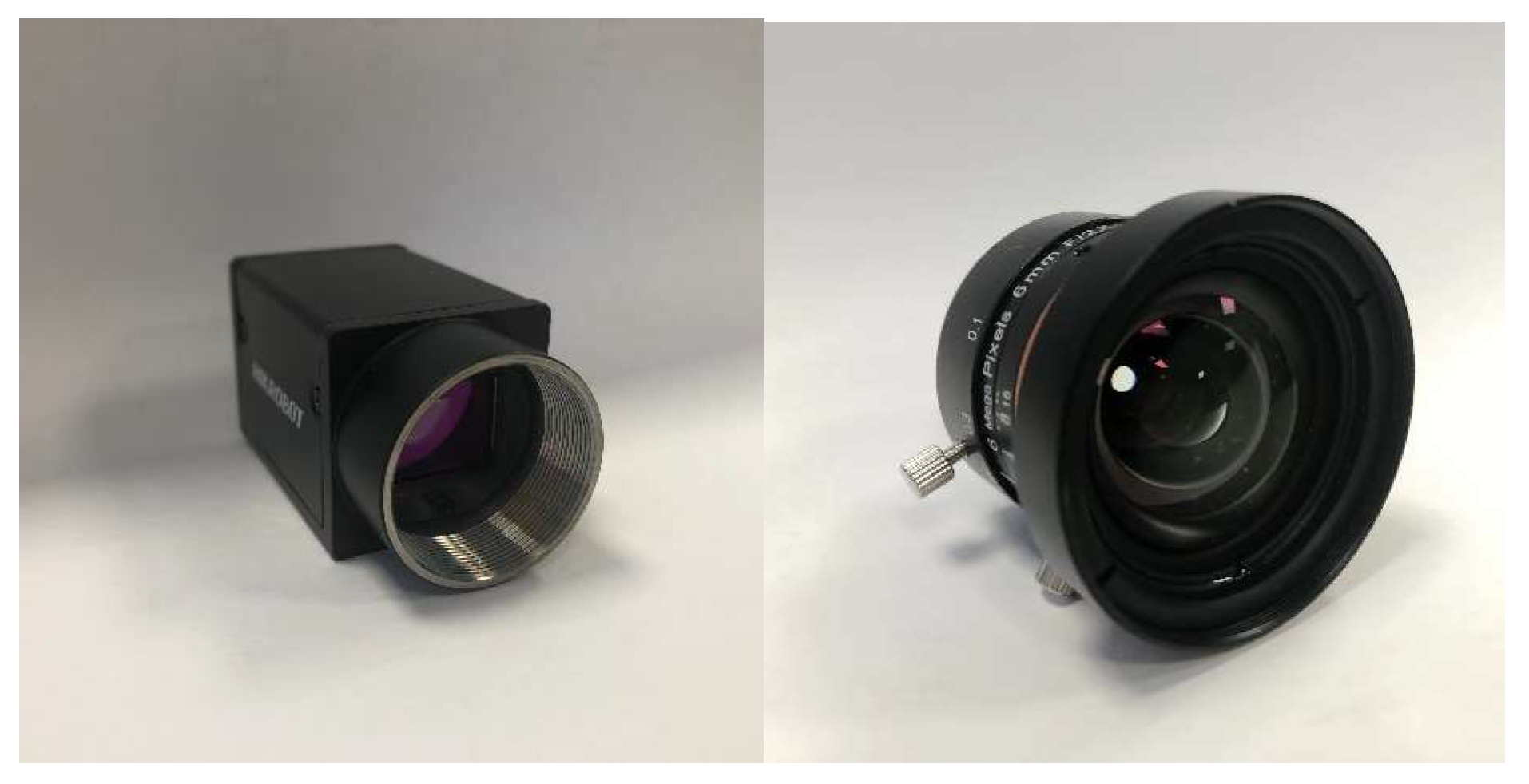
In this paper, we utilize an industrial camera with enhanced manufacturing accuracy and quality control as the visual sensor, along with an appropriate lens. The industrial camera is a Hikvision area-array CMOS camera, model MV-CE013-50GC and they are shown in Figure 8.
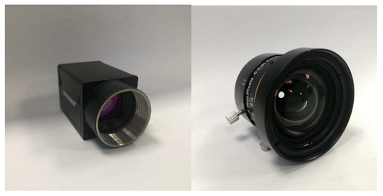
Figure 8.
Industrial camera and lens.
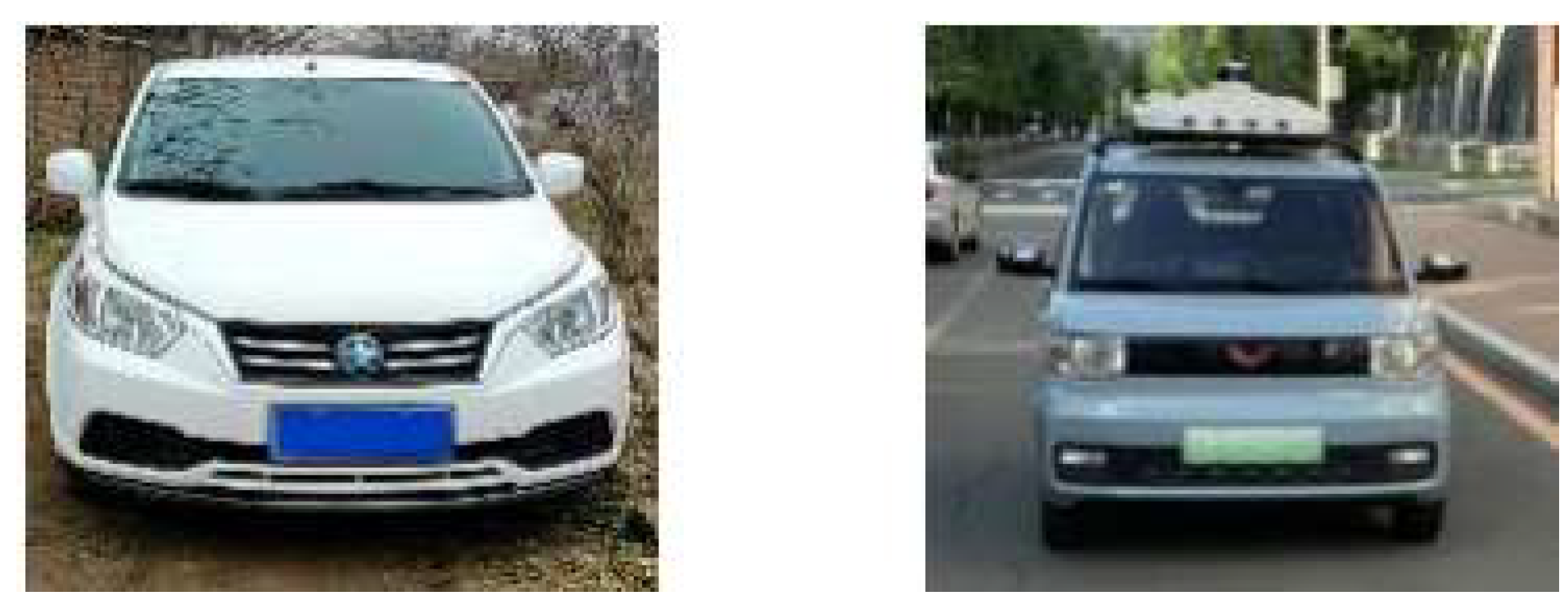
The vehicles used for data collection and real-world testing are Dongfeng Nissan Qichen R50 and Wuling Hongguang MINIEV. Figure 9 and Table 2 show the experimental vehicle and corresponding parameters, respectively. To enable convenient sensor installation while minimizing the effects of low temperature, the camera was horizontally mounted below the windshield, aligned with the vehicle’s center axis and placed in the center console.

Figure 9.
Experimental vehicles.
Table 2.
Experimental vehicle parameters.
5.1. Experiment of Drivable Area Detection Algorithm based on Lightweight Neural Network
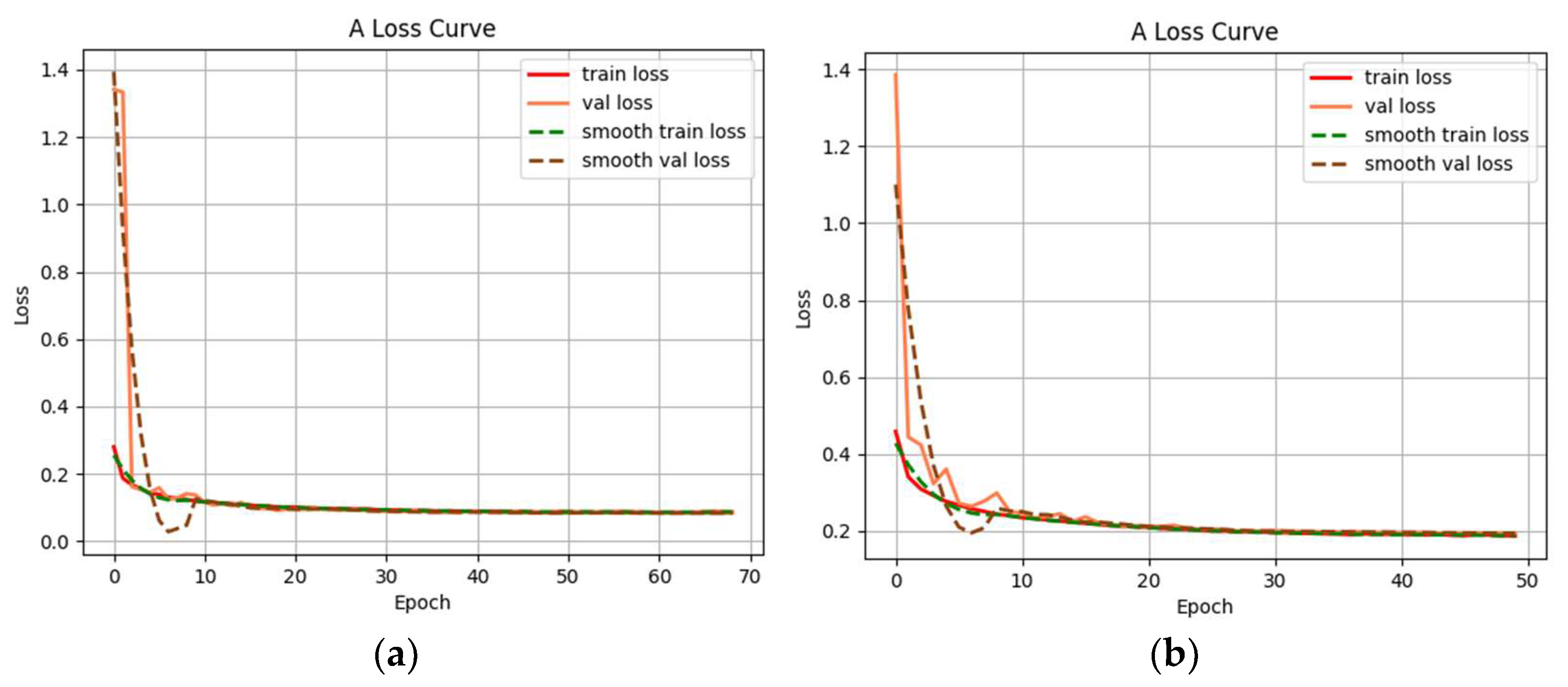
In this paper, three datasets were constructed: the global drivable area dataset, the road drivable area dataset, and the off-road environment drivable area dataset. These datasets are utilized for training and testing the network model separately. Additionally, a self-built small dataset is employed as an auxiliary validation set. Its purpose is to verify if the model can converge and demonstrate a certain level of generalizability. Simultaneously, this validation set helps assess the impact of different datasets on the network’s fitting ability. After the validation process, the final formal training is performed. The parameters are as follows: initial learning rate is set to 0.0001, decay ratio is 0.94, and the Adam optimizer is used; input image size is (3,469,469), automatic adjustment of the input image size is made through the internal interface, and the size of the network kernel parameters remains unchanged; batch size is 8, initial iteration number is 100, and single iteration data loading volume is adjusted based on the different datasets, using 10,000 as the base unit. Each dataset is randomly divided into multiple groups each time, and the training is validated by the group. Finally, the verification effect and loss function curve of the network model under three data sets are obtained, which are shown in Figure 10, Figure 11, Figure 12 and Figure 13.
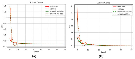
Figure 10.
Training model loss function graphs: (a) global training model loss function and (b) local training model loss function.
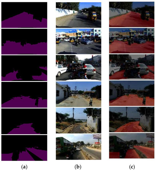
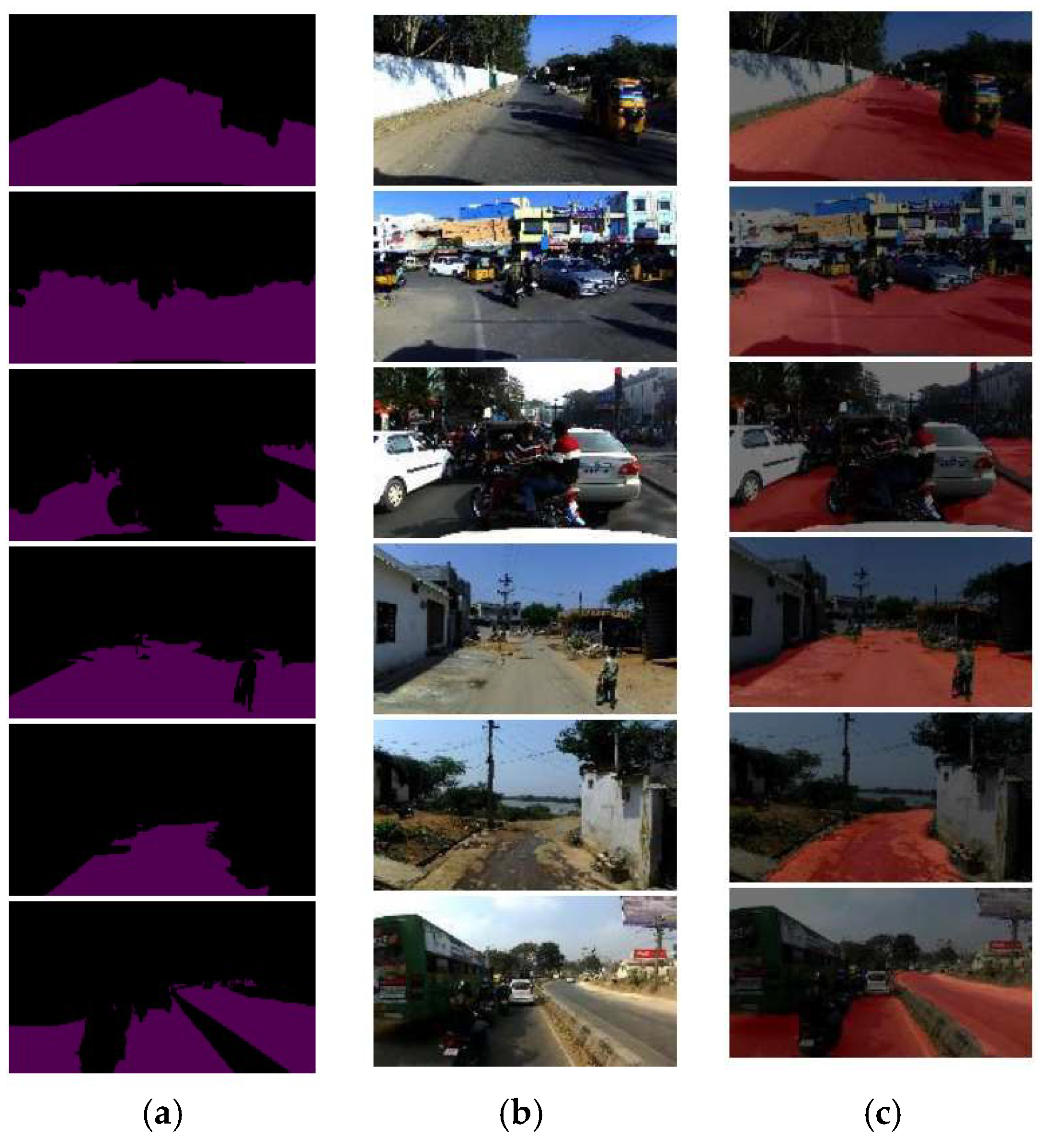
Figure 11.
Global training verification effect: (a) label of real value, (b) original images, and (c) global training model output.
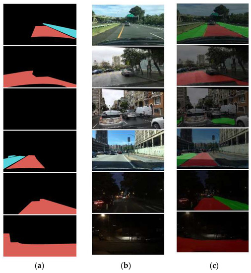
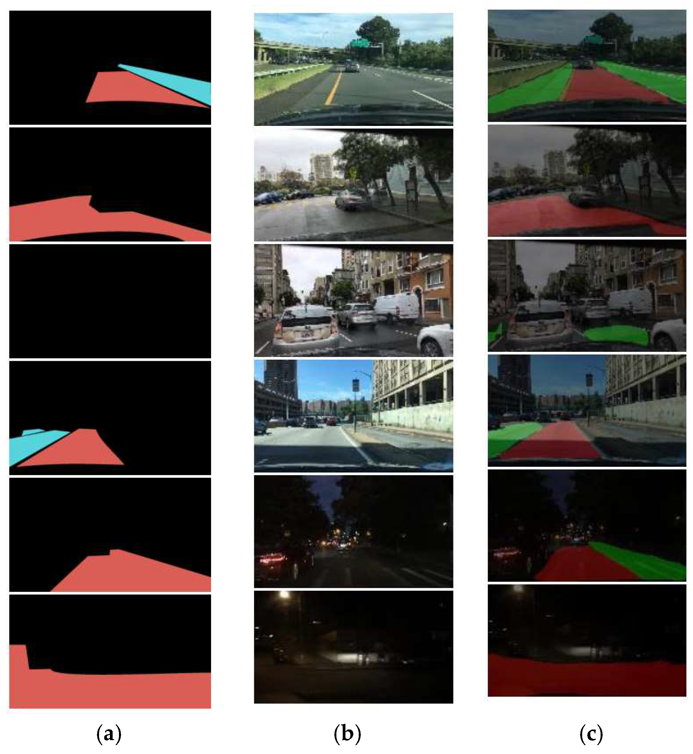
Figure 12.
Local training model verification effect: (a) label the real value, (b) original images, and (c) local training model output.
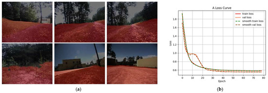
Figure 13.
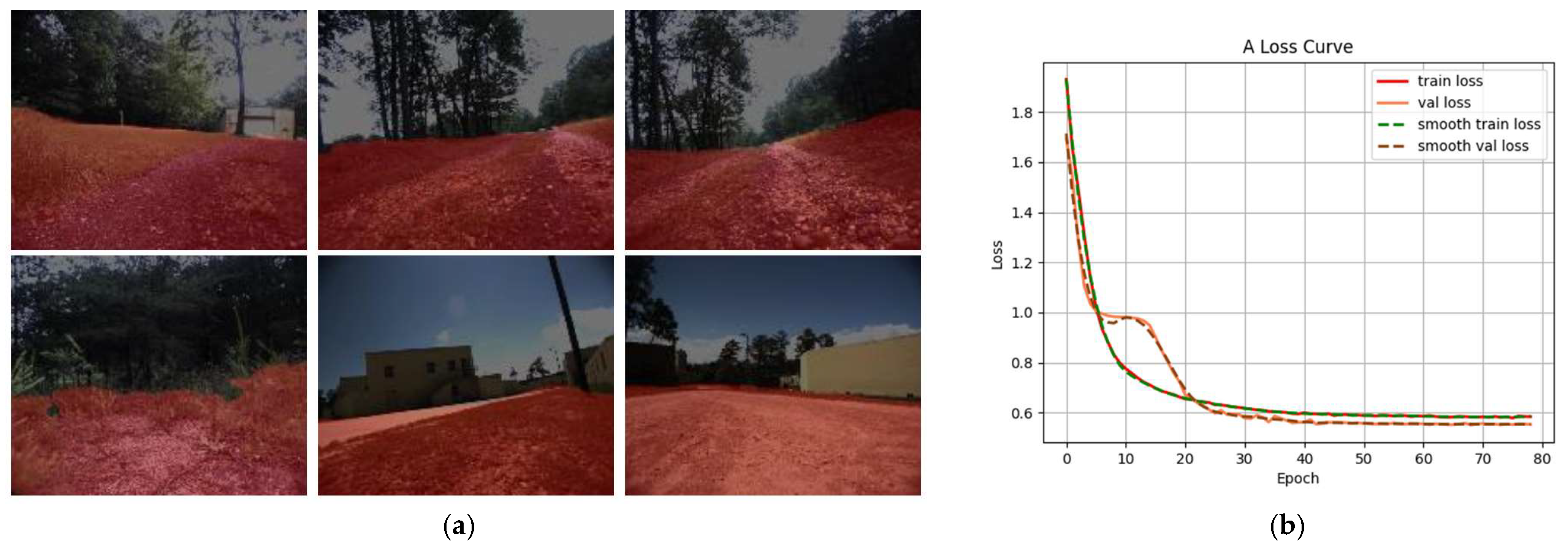
Cross-country training model verification effect: (a) cross-country training model validation results and (b) model loss function graph.
Figure 11 shows the validation effect of the global training model, labeled with the real value for the visualization of the modified mask file. The modified global drivable area includes asphalt road, dirt ground, stone ground, and sand ground. The elements of obstacles and other attributes are grouped into the background class. The area covered by the red mask in the validation effect figure is the drivable area identified by the network model. Figure 10a shows that the first 10 iterations of the network converge faster. Before reaching 70 iterations, due to the small change in the loss function of successive generations, the training is terminated in advance, and the final verification set loss function is stable at about 0.083. It is shown that the detection division of the drivable area is more stable, and the misclassification with the background area is smaller.
Figure 12 is the verification effect diagram using the local training model. The dataset is labeled for the differentiation of lane drivable areas on structured roads. The mask files provide labeled visualizations of real values for the current lane, and both lanes are divided into two types of areas: the current drivable area and the optional drivable area. Lane lines are not labeled; in the environment where lane lines cannot be identified, the road area will be considered the current drivable area. The area covered by the red mask in Figure 12a is the current drivable area identified by the network model, and the area covered by the green mask is the optional drivable area identified. It is shown that the trained network model maintains a good level of detection for structured roads, with a small difference from the real value, and the unlabeled part of the validation set also achieves the detection of roads in drivable areas. From Figure 10b, it is shown that the model successfully completes the training convergence. It is shown that the network model in this paper is backwards compatible with the lane structure detection of structured roads when trained with a suitable dataset.
In the initial stage of training with the off-road dataset, the dataset was labeled with the grass category into the drivable area for processing, and the final validation test results presented are shown in Figure 13a, where the detection effect is relatively stable. Most of all drivable ground structures are identified and labeled with red masks.
The training verification results and loss curves demonstrate that the proposed network structure can converge adequately and accomplish the drivable area identification task. The lower verification loss compared to the training loss is attributed to random deletion during training. This regularization approach slightly compromises network capability, while enhancing generalization. Random deletion is excluded in the validation and subsequent testing stages.
The network structure presented in this paper can achieve drivable area detection under complex situations on unstructured roads from a global perspective and can also finish drivable area detection for lane-based structured roads from a local perspective. Finally, it can be extended to off-road datasets to realize the detection of off-road drivable areas.
5.2. Network Model Test and Real Vehicle Experiments
The research content of this section is to apply the neural network model to identify the drivable area in the test set and the actual scene and verify the feasibility and rationality of the network model. Test and real vehicle test results are shown in Figure 14, Figure 15, Figure 16 and Figure 17.
Figure 14 shows the detection effect of some test set data, including day and night, rain and snow environment. As seen in Figure 14a, the network model is able to identify the global drivable area. Figure 14b is the self-built test set of rain and snow, soil road, and other specific circumstances. The original data frame has no obvious pavement structure, and the features are relatively broken. The network model can still identify the target area to a certain extent, and the area division is close to the actual situation.
There are two reasons for the decreased detection effect in Figure 14b compared to (a). First, there is no obvious feature for network detection after the road surface is covered with snow, and there is snow on the boundary between the road and the area alongside the stone. The boundary between the two is blurred and disappeared, resulting in misjudgment. Second, there is a shortage of strongly correlated data in the dataset, and there are situations in which the correlation feature mapping is attributed to the background class during the learning process, causing the network to fully train for specific situations. For the latter reason, this paper uses the network model trained by the cross-country environment drivable area dataset for simple testing. Considering the unevenness of the road surface and the spatial information of some elements, the grass category is used as the drivable area for training. The model and the results are shown in Figure 15. It is shown that the detection effect has a relatively obvious improvement, but there is also a misjudgment of the vertical spatial structure to a certain extent, which shows the influence of the dataset structure on the generalization ability of the network model. It also shows that some of the data in the self-built test set of this paper are close to the off-road environment and need further improvement. In addition, it shows that the network model of this paper has a certain generalization ability after being trained by suitable datasets.

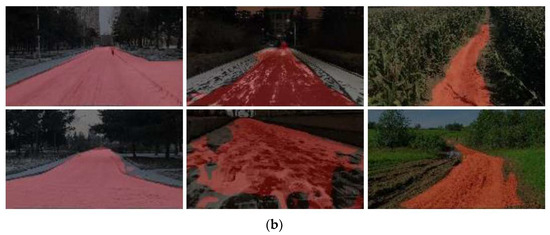
Figure 14.
Single-frame experimental effect of test set: (a) training effect of partial test set and (b) self-built test set that includes rain, snow, soil road, and other specific circumstances.
Figure 14.
Single-frame experimental effect of test set: (a) training effect of partial test set and (b) self-built test set that includes rain, snow, soil road, and other specific circumstances.
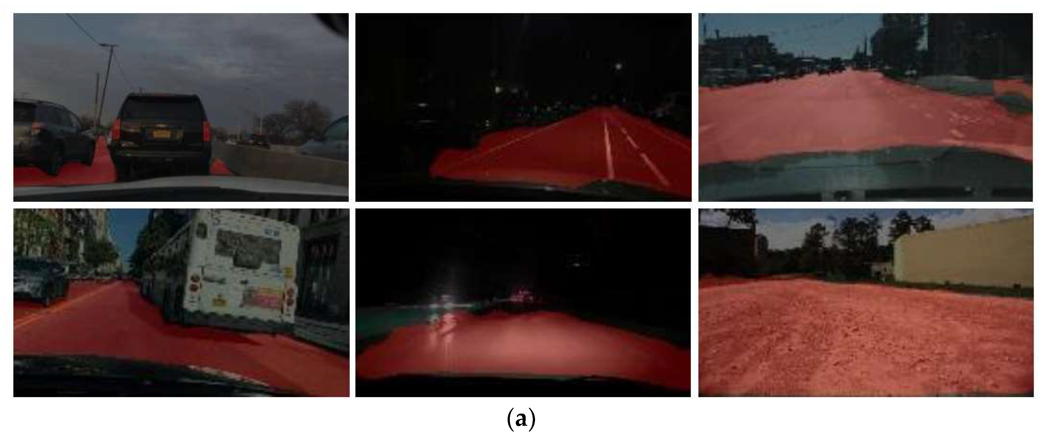

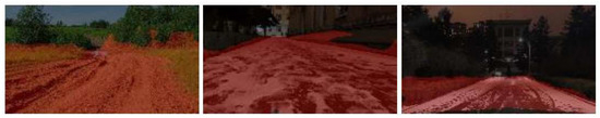
Figure 15.
Effect of cross-country dataset training model test set.
Figure 15.
Effect of cross-country dataset training model test set.

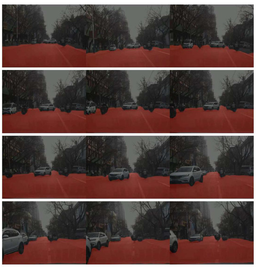
Figure 16.
Continuous frame effect of daytime real car experiment.
Figure 16.
Continuous frame effect of daytime real car experiment.

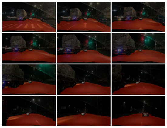
Figure 17.
Continuous frame effect of nighttime real car experiment.
Figure 17.
Continuous frame effect of nighttime real car experiment.
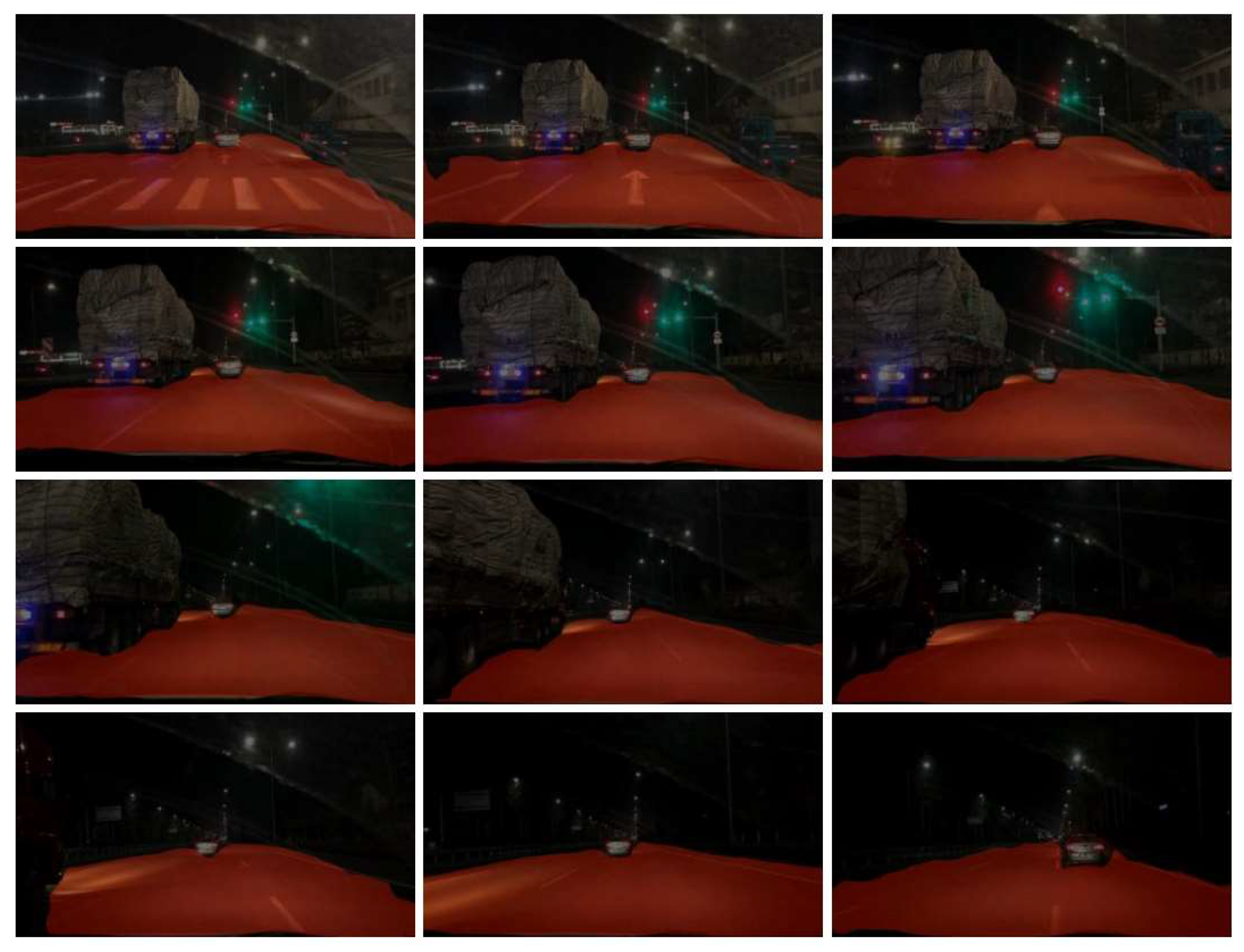
Figure 16 and Figure 17 show the intercepted frames of the real-time detection effect of the vehicle driving process under day and night conditions, respectively, which are intercepted according to the scene change amplitude to reflect the algorithm effect and not according to the fixed number of frames.
The training, testing, and real-vehicle experimental results demonstrate that the proposed network structure can effectively complete drivable area detection under varying conditions. It delivers robust performance on diverse data in the dataset. This indicates good generalization ability, feasibility, and applicability.
5.3. Network Model Evaluation
Starting from time cost, accuracy, and classification accuracy, this section compares and evaluates the lightweight network model proposed in this paper with ResNet and MobileNet. The time cost is based on the time required to process a single batch (milliseconds), and the time required to process a single iteration (seconds). The accuracy is the validation set accuracy, and the classification accuracy is the Mean Intersection over Union (MIoU) ratio. The validation set accuracy is calculated as the ratio of the total number of correctly classified pixel points p in a single data frame to the total number of pixel points N in the data frame:
The task of dividing the drivable area in this paper is a binary classification problem, and the target is the drivable area and the background class. Therefore, it is simplified here, and only the mean intersection over union ratio of the drivable area is calculated. The calculation form is as follows:
where p is the pixel point of the drivable area that is correctly classified, FN is the pixel point whose true value is the drivable area but is misclassified to the background, and FP is the pixel point whose true value is the background but is misclassified to the drivable area.
Model comparison training was performed in the Ubuntu environment, and the results are given in Table 3. The training data include 7000 random data frames, and the verification data frames are 1000. The ResNet50 network model selects a batch of 4, and the remaining two models are batched to 8. The iteration limit is 100 times, and the weight is saved once every 25 times. It is shown that compared with the other two networks, the time cost of the network structure in this paper is lower, and the accuracy and the mean intersection over union ratio have certain advantages. Compared with the typical deep network structure of ResNet50, the network structure of this paper still ensures a certain accuracy while the time cost is greatly reduced, which can better save system resources. Meanwhile, compared to the lightweight network MobileNetV2 [33,34], the network structure proposed in this paper also improves time consumption and accuracy.
Table 3.
Network model comparison.
6. Conclusions
In this paper, a lightweight convolutional neural network model was designed for the detection of drivable areas in complex situations of autonomous driving. This model is established based on a convolutional neural network for autonomous driving on unstructured roads. Furthermore, we design convolution modules based on residual network theory and deep separable convolution theory and parallel pooling modules based on computer multithreading and spatial pyramid model theory. In addition, we propose an improved network activation function, while considering the relationship between algorithm accuracy, computational consumption, and lightweight.
The model is trained and verified by the BDD100k dataset, RUGD dataset, and self-built dataset. The training results show that the MIoU of the model can reach 90.19, and the accuracy is 96.7%. It is shown that without losing accuracy, the running time is greatly reduced and the real-time performance is improved compared with the typical deep network structure of ResNet50.
In the future, for the case where the nighttime recognition effect is greatly affected by lighting conditions in the recognition results of the model in this article, it can be considered to use models such as conditional random fields for maximum posterior probability state inference. This could strengthen edge features and enhance the overall robustness of the scheme. We also consider introducing attention components into the network model.
Author Contributions
Y.Y. designed the method and wrote the paper; Y.L., P.W. and J.L. supervised the research and revised the manuscript; Y.H. wrote codes; and T.X. made the datasets. All authors have read and agreed to the published version of the manuscript.
Funding
This research was supported by the National Key Research and Development Program of China: 2021YFB2500704. The funder is the Ministry of Science and Technology of the People’s Republic of China, and the project represented by the fund number is to establish a dynamic analysis theory and design method for the full line control chassis based on the wheel motor action module and vehicle intelligence technology.
Data Availability Statement
The data may be available upon request from corresponding authors.
Conflicts of Interest
The authors declare no conflict of interest.
References
- Chen, L.-C.; Zhu, Y.; Papandreou, G.; Schroff, F.; Adam, H. Encoderdecoder with atrous separable convolution for semantic image segmentation. In Proceedings of the European Conference on Computer Vision (ECCV), Munich, Germany, 8–14 September 2018; pp. 801–818. [Google Scholar]
- Jung, C.R.; Kelber, C.R. Lane following and lane departure using a linear-parabolic model. Image Vis. Comput. 2005, 23, 1192–1202. [Google Scholar] [CrossRef]
- Chen, L.-C.; Papandreou, G.; Schroff, F.; Adam, H. Rethinking atrous convolution for semantic image segmentation. arXiv 2017. [Google Scholar] [CrossRef]
- Wang, G.; Zhang, B.; Wang, H.; Xu, L.; Li, Y.; Liu, Z. Detection of the drivable area on high-speed road via YOLACT. Signal Image Video Process. 2022, 16, 1623–1630. [Google Scholar] [CrossRef]
- Acun, O.; Küçükmanisa, A.; Genç, Y.; Urhan, O. D3NET (divide and detect drivable area net): Deep learning based drivable area detection and its embedded application. J. Real-Time Image Process. 2023, 20, 16. [Google Scholar] [CrossRef]
- Krizhevsky, A.; Sutskever, I.; Hinton, G.E. ImageNet Classification with Deep Convolutional Neural Networks. Commun. ACM 2017, 60, 84–90. [Google Scholar] [CrossRef]
- Alvarez, J.M.; Gevers, T.; LeCun, Y.; Lopez, A.M. Road Scene Segmentation from a Single Image. In Proceedings of the 12th European Conference on Computer Vision (ECCV), Florence, Italy, 7–13 October 2012; pp. 376–389. [Google Scholar]
- Long, J.; Shelhamer, E.; Darrell, T. Fully convolutional networks for semantic segmentation. In Proceedings of the IEEE conference on Computer Vision and Pattern Recognition, Boston, MA, USA, 7–12 June 2015; pp. 3431–3440. [Google Scholar]
- Mendes, C.C.T.; Fremont, V.; Wolf, D.F. Exploiting fully convolutional neural networks for fast road detection. In Proceedings of the IEEE International Conference on Robotics and Automation (ICRA), Stockholm, Sweden, 16–21 May 2016; pp. 3174–3179. [Google Scholar]
- Zhao, H.; Shi, J.; Qi, X.; Wang, X.; Jia, J. Pyramid scene parsing Network. In Proceedings of the IEEE Conference on Computer Vision and Pattern Recognition, Honolulu, HI, USA, 21–26 July 2017; pp. 2881–2890. [Google Scholar]
- Bilinski, P.; Prisacariu, V. Dense decoder shortcut connections for single-pass semantic segmentation. In Proceedings of the IEEE Conference on Computer Vision and Pattern Recognition, Salt Lake City, UT, USA, 18–22 June 2018; pp. 6596–6605. [Google Scholar]
- Yang, M.; Yu, K.; Zhang, C.; Li, Z.; Yang, K. Dense ASPP for Semantic Segmentation in Street Scenes. In Proceedings of the IEEE Conference on Computer Vision and Pattern Recognition, Salt Lake City, UT, USA, 18–22 June 2018; pp. 3684–3692. [Google Scholar]
- Li, X.; Zhao, H.; Han, L.; Tong, Y.; Tan, S.; Yang, K. Gated Fully Fusion for Semantic Segmentation. In Proceedings of the AAAI Conference on Artificial Intelligence, New York, NY, USA, 7–12 February 2020; pp. 11418–11425. [Google Scholar]
- Chen, J.; Wei, D.; Long, T.; Luo, T.; Wang, H. All-weather road drivable area segmentation method based on CycleGAN. Vis. Comput. 2022. [Google Scholar] [CrossRef]
- Yuan, Y.; Huang, L.; Guo, J.; Zhang, C.; Chen, X.; Wang, J. OCNet: Object Context Network for Scene Parsing. Int. J. Comput. Vis. (IJCV) 2021. [Google Scholar]
- Zhang, H.; Dana, K.; Shi, J.; Zhang, Z.; Wang, X.; Tyagi, A.; Agrawal, A. Context encoding for semantic segmentation. In Proceedings of the IEEE Conference on Computer Vision and Pattern Recognition, Salt Lake City, UT, USA, 18–22 June 2018; pp. 7151–7160. [Google Scholar]
- Zhao, H.; Zhang, Y.; Liu, S.; Shi, J.; Loy, C.C.; Lin, D.; Jia, J. PSANet: Point-wise spatial attention network for scene parsing. In Proceedings of the European Conference on Computer Vision (ECCV), Munich, Germany, 8–14 September 2018; pp. 267–283. [Google Scholar]
- Huang, Z.; Wang, X.; Huang, L.; Huang, C.; Wei, Y.; Liu, W. CCNet: Criss-cross attention for semantic segmentation. In Proceedings of the IEEE International Conference on Computer Vision, Seoul, Republic of Korea, 27 October–2 November 2019; pp. 603–612. [Google Scholar]
- Zhu, Z.; Xu, M.; Bai, S.; Huang, T.; Bai, X. Asymmetric non-local neural networks for semantic segmentation. In Proceedings of the IEEE International Conference on Computer Vision, Seoul, Republic of Korea, 27 October–2 November 2019; pp. 593–602. [Google Scholar]
- Jin, Y.; Han, D.; Ko, H. Trseg: Transformer for semantic segmentation. Pattern Recognit. Lett. 2021, 148, 29–35. [Google Scholar] [CrossRef]
- Dosovitskiy, A.; Beyer, L.; Kolesnikov, A.; Weissenborn, D.; Zhai, X.; Unterthiner, T.; Dehghani, M.; Minderer, M.; Heigold, G.; Gelly, S.; et al. An Image is Worth 16 × 16 Words: Transformers for Image Recognition at Scale. In Proceedings of the International Conference on Learning Representations, Addis Ababa, Ethiopia, 26–30 April 2020. [Google Scholar]
- Srinivas, A.; Lin, T.Y.; Parmar, N.; Shlens, J.; Abbeel, P.; Vaswani, A. Bottleneck Transformers for Visual Recognition. In Proceedings of the IEEE Conference on Computer Vision and Pattern Recognition, Virtual, 19–25 June 2021; pp. 16514–16524. [Google Scholar]
- Heo, B.; Yun, S.; Han, D.; Chun, S.; Choe, J.; Oh, S.J. Rethinking Spatial Dimensions of Vision Transformers. In Proceedings of the IEEE International Conference on Computer Vision, Virtual, 19–25 June 2021; pp. 11916–11925. [Google Scholar]
- Carion, N.; Massa, F.; Synnaeve, G.; Usunier, N.; Kirillov, A.; Zagoruyko, S. End-to-End Object Detection with Transformers. In Proceedings of the European Conference on Computer Vision 2020, Glasgow, UK, 23–28 August 2020; Volume 12346, pp. 213–229. [Google Scholar]
- Touvron, H.; Cord, M.; Douze, M.; Massa, F.; Sablayrolles, A.; Jégou, H. Training data-efficient image transformers & distillation through attention. In Proceedings of the International Conference on Machine Learning, Virtual, 13–18 July 2020; pp. 10347–10357. [Google Scholar]
- Yuan, L.; Chen, Y.; Wang, T.; Yu, W.; Shi, Y.; Jiang, Z.H.; Tay, F.E.; Feng, J.; Yan, S. Tokens-to-Token ViT: Training Vision Transformers from Scratch on ImageNet. In Proceedings of the IEEE International Conference on Computer Vision, Virtual, 19–25 June 2021; pp. 558–567. [Google Scholar]
- Xiao, T.; Singh, M.; Mintun, E.; Darrell, T.; Dollár, P.; Girshick, R. Early Convolutions Help Transformers See Better. In Proceedings of the Annual Conference on Neural Information Processing Systems, Virtual, 6–14 December 2021. [Google Scholar]
- Rao, Y.; Zhao, W.; Liu, B.; Lu, J.; Zhou, J.; Hsieh, C.J. DynamicViT: Efficient Vision Transformers with Dynamic Token Sparsification. In Proceedings of the Advances in Neural Information Processing Systems, Virtual, 6–14 December 2021. [Google Scholar]
- Chen, C.F.; Fan, Q.; Panda, R. CrossViT: Cross-Attention Multi-Scale Vision Transformer for Image Classification. In Proceedings of the IEEE International Conference on Computer Vision, Virtual, 19–25 June 2021. [Google Scholar]
- Wang, W.; Xie, E.; Li, X.; Fan, D.P.; Song, K.; Liang, D.; Lu, T.; Luo, P.; Shao, L. Pyramid Vision Transformer: A Versatile Backbone for Dense Prediction without Convolutions. In Proceedings of the IEEE International Conference on Computer Vision, Virtual, 19–25 June 2021. [Google Scholar]
- Cordts, M.; Omran, M.; Ramos, S.; Rehfeld, T.; Enzweiler, M.; Benenson, R.; Franke, U.; Roth, S.; Schiele, B. The Cityscapes Dataset for Semantic Urban Scene Understanding. In Proceedings of the IEEE Conference on Computer Vision and Pattern Recognition (CVPR), Las Vegas, NV, USA, 27–30 June 2016; pp. 3213–3223. [Google Scholar]
- Zhou, B.; Zhao, H.; Puig, X.; Xiao, T.; Fidler, S.; Barriuso, A.; Torralba, A. Semantic Understanding of Scenes Through the ADE20K Dataset. Int. J. Comput. Vis. 2019, 127, 302–321. [Google Scholar] [CrossRef]
- Meng, L.; Xu, L.; Guo, J.Y. A MobileNetV2 Network Semantic Segmentation Algorithm Based on Improvement. Chin. J. Electron. 2020, 48, 1769. [Google Scholar]
- Sandler, M.; Howard, A.; Zhu, M.; Zhmoginov, A.; Chen, L.C. Mobilenetv2: Inverted residuals and linear bottlenecks. In Proceedings of the IEEE conference on Computer Vision and Pattern Recognition, Salt Lake City, UT, USA, 18–22 June 2018; pp. 4510–4520. [Google Scholar]
- Mehta, S.; Rastegari, M.; Caspi, A.; Shapiro, L.; Hajishirzi, H. Espnet: Efficient spatial pyramid of dilated convolutions for semantic segmentation. In Proceedings of the European Conference on Computer Vision (ECCV), Munich, Germany, 8–14 September 2018; pp. 552–568. [Google Scholar]
- Paszke, A.; Chaurasia, A.; Kim, S.; Culurciello, E. Enet: A deep neural network architecture for real-time semantic segmentation. arXiv 2016. [Google Scholar] [CrossRef]
- Zhang, X.; Du, B.; Wu, Z.; Wan, T. LAANet: Lightweight attention-guided asymmetric network for real-time semantic segmentation. Neural Comput. Appl. 2022, 34, 3573–3587. [Google Scholar] [CrossRef]
- Park, H.; Yoo, Y.; Seo, G.; Han, D.; Yun, S.; Kwak, N. Concentrated-comprehensive convolutions for lightweight semantic segmentation. arXiv 2018. [Google Scholar] [CrossRef]
- Ma, S.; An, J.B.; Yu, B. Real time image semantic segmentation algorithm based on improved DeepLabv2. Comput. Eng. Appl. 2020, 56, 157–164. [Google Scholar]
- Wang, M.; Liu, B.; Foroosh, H. Factorized Convolutional Neural Networks. In Proceedings of the IEEE International Conference on Computer Vision Workshops, Venice, Italy, 22–29 October 2017; pp. 545–553. [Google Scholar]
- Chollet, F. Xception: Deep Learning with Depthwise Separable Convolutions. In Proceedings of the IEEE Conference on Computer Vision and Pattern Recognition, Honolulu, HI, USA, 21–26 July 2017; pp. 1800–1807. [Google Scholar]
- Howard, A.G.; Zhu, M.; Chen, B.; Kalenichenko, D.; Wang, W.; Weyand, T.; Andreetto, M.; Adam, H. MobileNets: Efficient Convolutional Neural Networks for Mobile Vision Applications. arXiv 2017. [Google Scholar] [CrossRef]
- Yu, F.; Koltun, V. Multi-Scale Context Aggregation by Dilated Convolutions. In Proceedings of the International Conference on Learning Representations, San Juan, Puerto Rico, 2–4 May 2016. [Google Scholar]
- He, K.; Zhang, X.; Ren, S.; Sun, J. Delving Deep into Rectifiers: Surpassing Human-Level Performance on ImageNet Classification. In Proceedings of the 2015 IEEE International Conference on Computer Vision (ICCV), Santiago, Chile, 7–13 December 2015; pp. 1026–1034. [Google Scholar] [CrossRef]
- Maas, A.L.; Hannun, A.Y.; Ng, A.Y. Rectifier nonlinearities improve neural network acoustic models. In Proceedings of the 30th International Conference on Machine Learning, Atlanta, GA, USA, 16–21 June 2013; Volume 30. [Google Scholar]
- Yu, F.; Chen, H.; Wang, X.; Xian, W.; Chen, Y.; Liu, F.; Madhavan, V.; Darrell, T. BDD100K: A Diverse Driving Dataset for Heterogeneous Multitask Learning. In Proceedings of the IEEE/CVF Conference on Computer Vision and Pattern Recognition (CVPR), Seattle, WA, USA, 13–19 June 2020; pp. 2633–2642. [Google Scholar]
- Varma, G.; Subramanian, A.; Namboodiri, A.; Chandraker, M.; Jawahar, C.V. IDD: A Dataset for Exploring Problems of Autonomous Navigation in Unconstrained Environments. In Proceedings of the IEEE Winter Conference on Applications of Computer Vision (WACV), Waikoloa Village, HI, USA, 7–11 January 2019; pp. 1743–1751. [Google Scholar]
- Wigness, M.; Eum, S.; Rogers, J.G.; Han, D.; Kwon, H. A RUGD Dataset for Autonomous Navigation and Visual Perception in Unstructured Outdoor Environments. In Proceedings of the IEEE International Conference on Intelligent Robots and Systems (IROS), Macau, China, 3–8 November 2019; pp. 5000–5007. [Google Scholar]


Disclaimer/Publisher’s Note: The statements, opinions and data contained in all publications are solely those of the individual author(s) and contributor(s) and not of MDPI and/or the editor(s). MDPI and/or the editor(s) disclaim responsibility for any injury to people or property resulting from any ideas, methods, instructions or products referred to in the content. |
© 2023 by the authors. Licensee MDPI, Basel, Switzerland. This article is an open access article distributed under the terms and conditions of the Creative Commons Attribution (CC BY) license (https://creativecommons.org/licenses/by/4.0/).