FPN-SE-ResNet Model for Accurate Diagnosis of Kidney Tumors Using CT Images

Abstract

Kidney tumors are a significant health concern. Early detection and accurate segmentation of kidney tumors are crucial for timely and effective treatment, which can improve patient outcomes. Deep learning techniques, particularly Convolutional Neural Networks (CNNs), have shown great promise in medical image analysis, including identifying and segmenting kidney tumors. Computed tomography (CT) scans of kidneys aid in tumor assessment and morphology studies, employing semantic segmentation techniques for precise pixel-level identification of kidneys and surrounding anatomical structures. This paper proposes a Squeeze-and-Excitation-ResNet (SE-ResNet) model for segmentation by combining the encoder stage of SE-ResNet with the Feature Pyramid Network (FPN). The performance of the proposed SE-ResNet model is evaluated using the Intersection over Union (IoU) and F1-score metrics. Experimental results demonstrate that the SE-ResNet models achieve impressive IoU scores for background, kidney, and tumor segmentation, with mean IoU scores ranging from 0.988 to 0.981 for Seresnet50 and Seresnet18, respectively. Notably, Seresnet50 exhibits the highest IoU score for kidney segmentation. These findings suggest that SE-ResNet models accurately identify and segment regions of interest in CT images of renal carcinoma, with higher model versions generally exhibiting superior performance. The proposed Seresnet50 model is a good tool for accurate tumor detection and image classification, aiding medical professionals in early diagnosis and timely intervention.

1. Introduction

1.1. Diagnosis

Diagnosis is the medical process of identifying the cause and effect of a disease or disorder using logic, analytics, and experience. It involves analyzing a patient’s medical history and physical examination to inform diagnosis, influencing the doctor’s visit process. Diagnosis involves statistical classification evaluations and categorization of an individual’s condition into distinct categories for medical decisions regarding treatment and prognosis. A diagnostic opinion is often described as a disease or other condition. Diagnosis is a crucial aspect of clinical decision-making, often involving ambiguity and uncertainty due to the inherent nature of the medical field [1,2,3,4]. The disease consists of observable signs and symptoms that medical professionals must interpret. The diagnosis procedure involves interpretation, a complex decision-making process in general medicine to accurately understand a patient’s health problem [5]. Disease diagnosis is crucial for clinical decision-making, involving subjective and objective factors. An accurate and prompt diagnosis is essential in determining a disease or disorder. A definitive diagnosis must be established before a treatment plan can be developed [6]. Diagnosis is a complex and challenging process for healthcare professionals, requiring them to consider multiple factors and circumstances. They gather empirical data to manage patients’ problems and reduce diagnostic uncertainty, ultimately improving healthcare quality [6]. Disease diagnosis is ambiguous and complex due to patient susceptibility and the complexity of the medical process. Unintended errors can occur due to the ambiguous nature of the disease, patient information, and the inherent essence of medicine [7,8].

1.2. Computer-Aided Diagnosis

Numerous researchers have utilized computer-assisted methods to enhance disease diagnosis to aid physicians in making the most accurate decisions, as accurate diagnosis is a crucial aspect of healthcare subjects [9,10,11,12,13,14]. Computer-aided diagnosis (CAD) can be defined as a radiologist’s use of output from a computer analysis of medical images as a “second opinion” in detecting lesions and making diagnostic decisions. The radiologist can then make the definitive diagnosis and treatment decisions. Recently, At many screening sites and hospitals in the United States, CAD has become an integral element of the routine clinical work for detecting cancer on medical images. CAD is increasingly being utilized to detect and diagnose abnormalities in medical images from various imaging modalities, making it a crucial research topic in medical imaging and diagnostic radiology [15,16,17,18,19].

1.3. Medical Imaging

Medical imaging techniques like X-rays, MRI, and CT require subjective analysis by radiologists. With increasing techniques, manual analysis becomes time-consuming. Machine learning models mimic human visual perception, enabling the automatic classification of images as diagnostic aids. Advances in AI and computing hardware have made computer-assisted methods more powerful, making them useful for diagnosticians. Consequently, CAD has acquired theoretical and practical significance as a significant trend in medical science. Using computer vision to automatically analyze and process medical images has many distinct benefits [13,20,21,22]. Utilizing medical images like PET, SPECT, MRI, and CT offers vital insights into head and neck cancer’s dimensions, site, structure, and metabolism [23]. Navigating clinical outcome prediction proves intricate yet pivotal for guiding treatment strategies [24]. In contrast to standard regression tasks like predicting clinical scores, clinical outcome prediction presents greater complexity due to survival data censoring, causing event times to be indeterminate for certain patients [25]. Accurate kidney tumor segmentation is pivotal in advancing kidney tumor diagnosis and treatment strategies through early detection, treatment planning, and risk assessment. However, real-time medical image analysis faces challenges like poor image quality, diverse protocols, and patient variations. Modern hardware’s computational power enables rapid analysis and processing, preventing fatigue and cognitive issues. Computer technologies facilitate data transmission, enabling accurate diagnosis of patients in remote areas. Machine learning algorithms and artificial intelligence classifiers improve prediction accuracy for kidney stone patients [20]. Since the introduction of the first (CNN) (LeNet-5 [26]) in 1989, CNNs exhibited exceptional performance in medical image processing [27,28]. The evolution of these models has also contributed to the precision of CAD techniques [17,29].

1.4. Convolutional Neural Network

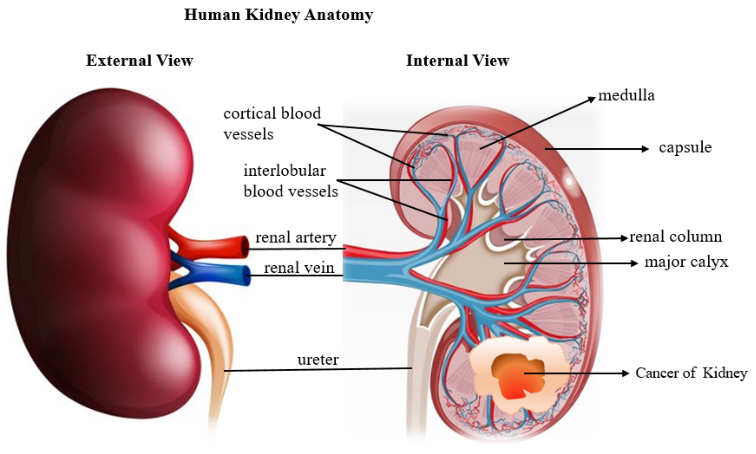
(CNN) has accomplished some outstanding feats. In the area of deep learning, it has grown to be one of the most representative neural networks. People have been able to do things previously thought impossible, like facial recognition, driverless automobiles, self-service supermarkets, and intelligent medical treatments, because of computer vision based on CNN [30]. Recent developments in deep convolutional neural networks (CNNs) have showcased their exceptional capabilities in mastering segmentation tasks across various imaging modalities and for diverse anatomical structures, e.g., prostate [31,32], heart [33,34], brain [35,36], head and neck [37,38], and COVID-19 [39]. The domain of automated medical image segmentation has witnessed remarkable advancements, reaching the pinnacle of performance through the utilization of deep learning and convolutional neural networks (CNNs) [27]. Over the past few years, convolutional neural network (CNN) based models for medical image segmentation have garnered substantial prowess, rivalling the performance levels achieved by radiologists [27,40]. However, these models have functioned as autonomous applications, tailored with refined architectures, preprocessing methodologies, data augmentation strategies, and metrics meticulously crafted to suit the distinct characteristics of their datasets and corresponding segmentation challenges [41]. Convolutional neural networks (CNNs) have emerged as the predominant deep learning model for organ and lesion segmentation tasks [42].

1.5. Kidney Cancer

The kidneys in the abdominal region are essential for bodily functions, containing connective tissue and fat. They dispose of metabolized compounds, maintain water and salt balance, and produce hormones for red blood cell production and blood pressure regulation. Figure 1 presents a visual depiction of the human kidneys. However, risk factors like smoking, obesity, and hypertension can compromise kidney function, leading to kidney cancer. DNA alterations can induce kidney cells to deviate from their fundamental role. Early detection is crucial for successful treatment and increased survival chances. Medical imaging tools like CT reveal the complex abdominal interior structure, often used for early-stage cancer detection [43,44]. Renal cancer ranks tenth globally, with a significant increase in individuals. In the US, 2023 projections predict 81,800 new RC diagnoses, resulting in 14,890 deaths [45]. Renal cancer is a diverse group of tumors originating from different kidney cell types, with renal cell carcinoma (RCC) being the most aggressive form, accounting for 70%. of all RC cases [46]. The prevalent subtypes of renal cell carcinomas (RCCs) encompass clear cell, chromophobe, oncocytoma, papillary, and other RCC subcategories. Accurate classification of histological subtypes within renal cell carcinoma is paramount to prevent unnecessary biopsies or surgeries [47]. By the World Health Organization (WHO) [48], The classification of RCC subtypes is of great importance as each type has its prognosis [48]. Conventional diagnostic methods may lead to misclassification of benign lesions like angiomyolipoma (AML) and oncocytoma (ONC) as RCC [49]. Incorrectly identifying benign lesions can lead to unwarranted surgical interventions, with 15–20. of tumors surgically removed with a preoperative RCC diagnosis potentially being angiomyolipoma (AML) [50]. Early and accurate diagnosis of renal tumors is crucial for treatment. Conventional tests like CBC, urinalysis, and blood assays can hint at RC but do not provide precise diagnoses or differentiate between subtypes, grades, or stages. Therefore, biopsy remains the ultimate benchmark for definitive RC diagnosis, as it accurately quantifies red blood cells, identifies blood, bacteria, or malignant cells, and gauges renal function [45]. Deep learning is a powerful machine learning technology that can autonomously acquire various features and patterns without human intervention [51,52]. DL has revolutionized prognostic models for early tumor detection using pattern analysis techniques, demonstrating superior performance over conventional machine learning due to its exceptional precision in delivering results [53]. Object detection, a technique used in image processing, has gained significant interest in medical radiology due to its focus on extracting valuable insights from images. This concept includes single-class and multiclass object detection, crucial in identifying object categories [54]. DL methodologies have significantly improved performance and automated segmentation models, especially with the latest advancements in convolutional neural networks (CNNs) [52,55]. CNNs are ideal for medical imaging because they can discern nuanced details. The SE-ResNet architecture enhances feature representation, highlighting relevant image structures and enabling CNNs to outperform traditional methods for more precise and efficient segmentation. In this study, the investigation delves into the utilization of five architectures from the SE-ResNet lineage. Additionally, the study involves a comparison of outcomes across different SE-ResNet backbones.

1.6. Current Methods

Numerous DL techniques for kidney segmentation have been created utilizing (CNNs). In reference [56], The proposed 3D fully convolutional network uses a pyramid combining unit and progressively improved feature unit, evaluated using a specific dataset with an average Dice coefficient of 0.931%, by Yang et al. Cruz et al. [57] AlexNet was utilized as a classifier to distinguish non-kidney CT slices from kidney slices to prevent segment discontinuity, and a phase of recovery was implemented. Later, in initial segmentation by a 2D U-Net architecture, the CCL method decreased the number of false-positive predictions. A local test dataset produced a Dice coefficient degree of 96.33% for the (KiTS19) dataset. Hou et al. [58] Instead of aggregating operations, dilated convolution blocks were utilized in a three-stage 3D U-Net. Due to the three phases within the 3D U-Net, input images comprised low-resolution, high-resolution, and trimmed images. A hybrid reduction function comprised of (DC) and a weighted cross-entropy was employed. On the KiTS19 dataset, the technique attained an average Dice score(DS) of 0.9674. Türk et al. [59] A hybrid 3D V-Net model using ResNet++ output layer architecture outperformed the original V-Net with a 0.97 Dice coefficient. Training is challenging due to time and computing resources, and lightweight 2D models are preferred for kidney segmentation assignments.

1.7. Problem Description

Methods of segmentation based on the proximity of pixels are region-based. The authors in reference [60] Propose coarse-to-fine kidney segmentation using kernel fact hunt and adaptive region-growing, modifying attention construction limitations. Erdt et al. [61] Utilizing native restraints prevents adjacent organs from affecting deformable models. Khalifa et al. [62] The level-set procedure generates a deformable model, probabilistic form, voxel communication, and stochastic haste purpose for segmentation presentation; the atlas-based technique uses functional diagrams for orientation and consistent comments. Yang et al. [63] Two-step multi-atlas image registration technique for renal segmentation using random forest and machine learning classifier. Cu-ingnet et al. [64] Random forest algorithm classifies dynamic contrast-enhanced images. Jinet et al. [65,66] Earlier attempts to resolve this issue have shown result promise. This study uses five lightweight architectures from the SE-ResNet family designed to optimize resources while maintaining high precision. These architectures are valuable for achieving comparable outcomes to current methods while requiring less space and training time. The study evaluates SE-ResNets’ ability to classify kidney tumor images using F1-score, IoU scores, and the KiTs 19 dataset.

1.8. Paper Structure

This paper is organized into different sections. Section 2, the Materials and Methods, discusses the Dataset and provides information on the framework used in this study. Section 3, Results and Discussion. Finally, Section 4 discusses the insights gained from this study and concludes the paper.

2. Materials and Methods

This paper uses part of the KiTS19 dataset, including CT scans of abdomens with kidney tumors, to train and evaluate segmentation algorithms for detecting and delineating kidney tumours. The study employs Intersection over Union (IoU) and F1-score metrics to assess the method’s accuracy and effectiveness. The primary objective is to achieve accurate and efficient identification and delineation of kidney tumors and kidneys within CT images, supporting clinicians in diagnosing and monitoring kidney tumors and improving patient care and treatment outcomes.

2.1. Dataset

The facts for the examination are obtained from KiTS19 [67]. It is a dataset for training and testing machine learning models that comprises CT scans and corresponding annotations for kidney tumor segmentation. It is a widely utilized benchmark dataset for assessing the performance of medical image segmentation models for renal tumors. The testing and challenging training datasets consist of 210 CT volumes of the abdomen. Each volume’s imaging and ground truth labels are provided in Neuroimaging Informative Technology Informative (DICOM) format with shape (number of segments, height, and width). It is located on Kaggle at “https://www.kaggle.com/competitions/body-morphometry-kidney-and-tumor/data/” (accessed on 1 March 2023) (Who used the original data in reference [67]) The dataset consists of segments ranging in size from 29 to 1059 pixels and grayscale images measuring 512 × 512 pixels. The characteristics of the experimental dataset are provided in

Table 1. Dataset Properties Used for the Experimentation are cited.

Properties	Values
Number of all Image	7899
Number of Training Images	5841
Number of Validation Images	1027
Number of Testing Images	1031
Image format	Png
Modality	CT

below. This study utilized a subset of the dataset of 7899 PNG images.

2.2. Preprocessing

Indeed, preprocessing is essential to the classification of CT images. Typically, CT images are stained with various dyes to emphasize various structures and characteristics, and they can vary considerably in terms of staining intensity, colour, and texture. Therefore, preprocessing is required to improve image quality and consistency and eliminate noise and artefacts that could interfere with the classification process [68]. In contrast, Convolutional neural networks (CNNs) are designed to handle smaller inputs, requiring reduced image resolution to maintain essential details. Preprocessing processes and resizing or downsampling CT images are crucial for CNNs to process them effectively. The input image size significantly impacts the network’s efficacy, so reducing the resolution while maintaining essential characteristics and structures is essential. Downsampling methods, such as bilinear or nearest-neighbor interpolation, or more complex methods, such as wavelet-based or deep learning-based approaches, can achieve this. Within this range, The initial step in processing these images is to convert them from DICOM to PNG. DICOM images are converted to PNG format during preprocessing through a standardized transformation process. This conversion maintains image quality. It is located on Kaggle at “https://github.com/hwanseung2/kidney-tumor-segmentation/blob/main/2Dsegmentation-fastai.ipynb” (accessed on 5 March 2023). Moreover, put images in size 128 × 128.

2.3. Feature Pyramid Network

Feature pyramids involve the integration of high-level feature maps spanning various scales, collaborating harmoniously with backbone networks. This synergy yields enhanced and equitable performance across multiple scales, augmenting object detection capabilities [69,70,71], and semantic segmentation [71,72,73]. The primary objective of object detection, a fundamental facet of computer vision, entails identifying the positions and categorizing objects within an image. This pursuit lays the foundation for other related tasks, including human pose estimation, expanding the scope of its utility [74]. FPN [70], Feature Pyramid Network (FPN) is a groundbreaking method in object detection using convolutional neural networks. It uses multi-scale feature data to enhance accuracy, particularly in detecting small-scale objects. The FPN’s core concept is a feature pyramid that scales features across different tiers, allowing for a more detailed representation of lower-level information. This approach surpasses the granularity of higher-level features, allowing for more accurate detection of smaller objects. FPN’s versatility makes it ideal for identifying and discerning small target objects, demonstrating its remarkable efficacy. The FPN algorithm is a trilateral process consisting of an initial traversal through a bottom-up convolutional neural network, an iterative descent from a top-down perspective, and a pivotal lateral connection that links features with their counterparts. The bottom-up phase in convolutional neural networks involves the gradual evolution of feature map dimensions as data moves forward. This dynamic fluctuation leads to the stratification of layers into discrete stages, where layers that maintain the feature map’s size coalesce into a stage. This categorization helps assign unique attributes to each extraction task, which crystallizes as the final output from each step. This process creates a composite feature pyramid, with diverse characteristics from each stage contributing to a hierarchical ensemble. The top-down progression entails an intricate movement accomplished through Upsampling, a technique consistently reliant on the interpolation principle. In this context, Upsampling orchestrates the magnification of the original image, artfully infusing new elements between pixels. This augmentation is executed via a judicious interpolation algorithm woven around the original image’s pixel configuration bedrock. It is paramount to underscore that the feature map ensuing from this Upsampling operation retains an identical dimension as the feature map is immediately contiguous in the layered hierarchy. This study compares various encoder configurations using EfficientNet, U-Net, and SE-ResNets lineages, examining their performance and result.

2.4. SE-ResNets

In SE-ResNets, add a module to residual blocks after activation, enabling access to feature maps and focusing on significant features early in the network [75]. The combination of SE block and ResNet models significantly improves image classification performance, especially for iconic and abstract images. SE blocks selectively focus on key features, acquiring more discriminative representations and improving prediction accuracy. SE-ResNet models consistently demonstrate state-of-the-art performance in benchmark datasets like ImageNet and CIFAR-10 [75]. For instance, SE-ResNet152 outperformed ResNet152 in the ImageNet dataset with a top-1 accuracy of 82.63% [75]. SE-ResNet models performed better than ResNet models on the CIFAR-10 dataset, with SE-ResNet152 achieving a test accuracy of 96.54% compared to 94.54% for ResNet152. Recommended ASC system. Note that all accuracy measurements were conducted using a four-ensemble model. The accuracy of ResNet-rev improved as the number of layers increased. Specifically, ResNet(152)-rev improved relative class performance by 12.5% compared to the baseline. Next, the classwise accuracy of SE-ResNet-rev was evaluated and found to be superior to that of ResNet-rev at 152 layers. Finally, WaveGAN was used to augment the training data. Therefore, the classwise accuracy of SE-ResNet(152) rev-aug was 70.5%. This was because the sampled wave may have needed to be more accurate, and the GAN-based generator and discriminator may have needed to be more adequately trained [76].

2.5. SE-ResNet + FPN Network

Using convolutional neural networks (CNNs) for semantic image attributes requires a strategic approach. CNNs, a vital tool in deep learning methodologies, follow a standardized structural composition for feature extraction. This architecture involves convolutional and pooling layers, resulting in a plain network. Examples of this genre include AlexNet and VGG. CNNs are known for their depth and intricate calculations, making them a powerful tool [77,78]. A deep-network structure for the plain network can be used to obtain a high-level feature map of each image. After downsampling, the minor details shrink or even vanish. There needs to be more data available, though, about high-resolution feature maps without downsampling. It does not allow for the easy extraction and characterization of the intricate tiny characteristics needed for our dataset. Feature pyramid network’s (FPN) concept of feature pyramids served as inspiration [70]. Backbone branch: higher layers of representation amplify input characteristics crucial for discriminating and reducing unimportant variations to extract better features for the classification task [79]. Hence, we adopted SE-ResNet as our backbone to secure ample depth for rich semantic extraction due to its shortcut-connected, gradient-efficient residual mapping. The FPN framework focuses on creating a comprehensive feature pyramid with high semantic content, using a multi-pronged approach with bottom-up and top-down pathways interlinked through lateral connections.

2.6. Evaluation Metrics

F1-score and IoU were used in the study to evaluate the segmentation results. The Dice Similarity Coefficient (DSC), also known as the F1-score or Srensen-Dice index, and the Intersection-over-Union (IoU), also known as the Jaccard index or Jaccard similarity coefficient. The IoU penalizes under and over-segmentation more than the DSC, even though the DSC is defined as the harmonic mean between sensitivity and precision. The DSC is a widely used metric to assess the segmentation performance using the provided ground truth in medical images, although both scores are valid metrics [80,81]. These dimensions are expressed as follow [13]:

$$F1-score=\frac{2TP}{(TP+FP)+(TP+FN)}$$

(1)

$$IoU=\frac{TP}{(TP+FP+FN)}$$

(2)

2.7. Loss Function

The medical image predominantly comprises a minor fraction dedicated to lesion regions, exacerbating the pronounced disparity in positive and negative sample distribution. This imbalance notably impacts the accuracy of lesion region segmentation. In 2017, Tsung Yi Lin introduced focal loss as a potential remedy for this concern [82]. In object detection, focal loss was introduced to tackle the imbalanced positive and negative sample distribution challenge. In the context of medical image segmentation, where labels are influenced by clinical expertise, the potential for erroneous annotations exists. The focal loss conducts pixel-level classification, rendering the impact of these inaccuracies substantial within the network. While focal loss has its constraints, its effectiveness in mitigating imbalanced samples makes it a promising candidate for addressing similar issues in medical image segmentation. Pastor-Pellicer initially introduced the Dice loss function [83]. The Dice loss, tailored for object segmentation utilizing the Dice similarity coefficient (DSC), emerges as a dedicated choice, particularly prevalent in medical segmentation endeavors [84]. Medical imagery often has a small region of interest, leading to a learning process skewed toward background predictions. Because the region of interest only makes up a small portion of the scan, this can affect the accurate recognition of foreground regions, frequently leading to incomplete detection or potential omissions [85].

2.8. Proposed Solution

The study introduces a methodology that utilizes the KiTS19 database to accurately segment tumors and kidneys on CT slices [67]. The method involves two primary stages: data preparation, where CT volumes are scaled and normalized to enhance data consistency and quality, and segmentation using a SE-ResNet FPN model to delineate tumors and kidneys accurately. After converting the volumes from DICOM to PNG format, the segmentation process employs a SE-ResNet FPN model to delineate the kidneys and tumor, streamlining the segmentation stage. The SE-ResNet family is an excellent choice for the encoder component, while the FPN acts as the decoder, utilizing multiscale feature maps. The method typically calculates intersection-over-union (IoU) scores for various predictions and selects the segmentation with the IoU score and F1 score to determine the optimal segmentation. The segmentation models library is an open-source resource comprising cutting-edge deep-learning models designed for image segmentation tasks, encompassing state-of-the-art architectures for semantic, instance, and panoptic segmentation, such as U-Net, PSPNet, FPN, and LinkNet. The segmentation models library offers the advantage of transfer learning and fine-tuning on custom datasets, making it a valuable tool for researchers and practitioners in image segmentation tasks. It is located on GitHub at “https://github.com/qubvel/segmentationmodels” (accessed on 25 March 2023).

2.8.1. Backbone Architectures

The backbones of feature extraction networks compute image input features, and selecting the optimal network is crucial for objective task performance and DL model computational complexity. Numerous backbone networks have been designed and implemented in various DL models [86]. Further research is needed to compare feature extraction networks for Deep Learning applications [86]. This study evaluates five existing feature extraction backbone networks for a single model to determine the most effective combination. Unsuitable backbones can degrade performance, be computationally expensive, and be complex. The study aims to improve model performance and reduce computational costs. Figure 2 summarizes the categories (family) and names of the backbones.

2.8.2. Methodology

In this work, semantic segmentation of renal tumors Combines a semantic segmentation model and five feature extraction networks, which results in the proposed methodology. This modular design aims to determine the optimal segmentation solution for kidney tumors. Additionally, The optimal Loss function is investigated and evaluated from both model and backbone perspectives, and the methodology is proposed, as shown in Figure 3.

The proposed segmentation architecture combines a semantic segmentation model with five feature extraction networks, resulting in output segmentation images and numerical experimental results.

2.9. Implementation

In this paper, we implemented all algorithms using Python 3.9.16 on a DELL CORE i5 personal computer with the support of Anaconda and Jupyter. Initially sized at 512 × 512 pixels, the original images underwent uniform resizing to (128 × 128) pixels, serving as the segmentation model’s input. Focus in this section revolves around constructing five models from the SE-ResNets family, namely, `Seresnet18’, `Seresnet34’, `Seresnet50’, `Seresnet101’ and `Seresnet152’, employing the FPN (Feature Pyramid Network) architecture. This approach aims to leverage the capabilities of the SE-ResNets and the benefits of the FPN framework to enhance the accuracy and efficiency of our segmentation model.

2.10. Model Setup

Every model undergoes training for a total of 50 epochs. In order to prevent overfitting, the training process concludes when the validation loss stays at or above 0.0001. All backbone architectures are initialized with weights pre-trained on ImageNet to expedite convergence. The specifics of baseline model configurations and hyperparameters for all deep learning models are provided in

Table 2. Models’ hyperparameter setup.

Hyperparameter	Settings
Activation	`softmax’
Optimizer	Adam
Loss function	Focal Loss, Dice Loss
Learning rate	0.0001
Batch size	32
Epochs	50
Metrics	IoU, F1-score
Input images size	128 × 128

.

3. Results and Discussion

This section discusses assembling the five models, Seresnet18, Seresnet34, Seresnet50, Seresnet101, and Seresnet152, using FPN architecture. To train all models using SE-ResNet PFN architecture.

3.1. Experimental Results

In

Table 3. Outcomes of the Ensemble Model of Seresnet50.

IoU Scores	Obtained Values
Background IoU Score	0.999
Kidney IoU Score	0.980
Tumor IoU Score	0.984
Mean IoU Score	0.988

, the accuracy of the ensemble model of Seresnet50 for Background, Kidney, Kidney Tumor, and Mean IoU outcomes is presented.

The accuracy of Seresnet50 is assessed through IoU scores, which gauge the concordance between predicted and actual segments. Elevated scores signify strong correspondence between predictions and actual structures in medical images, indicative of proficient identification and segmentation. High IoU scores, for instance, Background 0.999, Kidney 0.980, and Tumor 0.984 underscore the model’s precision in outlining these specific areas.

3.2. Discussion

3.2.1. Result Analysis

ImageNet assessed and optimized best-performing models, despite patch-wise classification using local features [48]. This research investigates the architecture’s ability to extract global features from CT images of renal cancer and classify unseen images, revealing that extracting nuclei and tissue organization features is more valuable than nuclei-scale features for deciphering image classes.

Evaluated different models based on their performance and employed a metric called Mean IoU (Intersection over Union) to assess the accuracy of the models. The study compared several models based on the SE-ResNet architecture with FPN (Feature Pyramid Network) and presented the results in

Table 4. Results for the SE-ResNet with FPN Architectures Using Mean IoU.

SE-ResNet	Background	Kidney	Tumor	Mean
Seresnet18	0.999	0.972	0.971	0.981
Seresnet34	0.999	0.972	0.971	0.981
Seresnet50	0.999	0.980	0.984	0.988
Seresnet101	0.999	0.976	0.982	0.986
Seresnet152	0.999	0.979	0.984	0.987

. Each model was evaluated regarding background IoU score, kidney IoU score, tumor IoU score, and mean IoU score. The IoU scores indicate how well the models performed in segmenting different regions of the CT images. A higher IoU score signifies better performance, indicating higher overlap between the predicted and ground truth regions. The results demonstrate that all the SE-ResNet models achieved excellent IoU scores across the different categories. For example, the `Seresnet18’ model achieved a background IoU score of 0.999, a kidney IoU score of 0.972, a tumor IoU score of 0.971, and a mean IoU score of 0.981. Similarly, the other models, `Seresnet34’, `Seresnet50’,`Seresnet101’ and `Seresnet152,’ also achieved high IoU scores across the categories. Based on these results, it can be inferred that the SE-ResNet models with FPN architecture effectively extracted global features from CT images of renal cancer and utilized them to classify unseen images accurately. Figure 4 compares results for the SE-ResNet with FPN Architectures Using Mean IoU.

Table 5. Results for the SE-ResNet Accuracy IoU and F1-score Using Validation Images.

SE-ResNet	Loss	IoU Score	F1-Score
Seresnet18	0.753	0.979	0.989
Seresnet34	0.753	0.979	0.989
Seresnet50	0.752	0.987	0.993
Seresnet101	0.752	0.985	0.992
Seresnet152	0.752	0.986	0.993

presents the results of the SE-ResNet models in terms of accuracy and loss. IoU score (Intersection over Union) and F1-score using validation images for evaluation. These metrics provide insights into the performance of the models in terms of overall accuracy and their ability to accurately segment and classify objects in the images. The accuracy represents the percentage of correctly classified instances from the total instances in the validation dataset. In this case, the accuracy is measured by the loss value, which is inversely proportional to accuracy. Therefore, a lower loss value indicates higher accuracy. For all the SE-ResNet models, including `Seresnet18’, `Seresnet34’, `Seresnet50’, `Seresnet101’, and `Seresnet152’ the loss values are around 0.752, indicating good accuracy in the range of 75.2%. The IoU score, the Jaccard Index, measures the overlap between the predicted and ground truth segmentation. A higher IoU score indicates better performance in accurately identifying and localizing objects. The SE-ResNet models achieved high IoU scores, ranging from 0.979 to 0.987. For example, the `Seresnet18’ and ’Seresnet34’ models achieved an IoU score of 0.979, while ’Seresnet50’ achieved a slightly higher score of 0.987. Similarly, `Seresnet101’ and `Seresnet152’ achieved IoU scores of 0.985 and 0.986, respectively. These scores suggest that the models effectively segment the objects of interest in the validation images. The F1-score measures the models’ accuracy in terms of precision and recall. It considers both false positives and false negatives in the predictions. The SE-ResNet models achieved high F1- scores, ranging from 0.989 to 0.993. The scores indicate a high level of precision and recall in classifying the objects in the images, with `Seresnet50’, `Seresnet101’, and `Seresnet152’ achieving slightly higher scores compared to `Seresnet18’ and `Seresnet34’. These results demonstrate that the SE-ResNet models performed well in terms of accuracy, IoU score, and F1 score when evaluated on the validation images. They showcase the models’ ability to classify accurately and segment objects, indicating their potential usefulness in tasks such as image classification and object detection. SE-ResNet accuracy, IoU, F1-score, and loss results are shown in Figure 5.

3.2.2. Model Accuracy and Model Loss

The SE-ResNet model’s performance is evaluated using metrics like loss and IoU Score to minimize discrepancies between predicted and actual values. It measures the overlap between predicted bounding boxes and the ground truth, assessing accuracy in segmenting kidney tumors and kidneys. IoU Score measures the overlap between predicted and accurate segmentation, while the loss function quantifies the model’s performance in minimizing the error between predicted outputs and ground truth, optimizing segmentation results. In Figure 6 and Figure 7, Model accuracy and Model loss Seresnet50. Our strategies remained immune to overfitting issues due to the appropriate dataset.

The discussion on the performance evaluation of different versions of the SE-ResNet model in terms of loss and IoU score. Loss is a metric that measures how well the model minimizes the difference between predicted and actual values. IoU score, on the other hand, measures the overlap between the predicted bounding boxes and the ground truth bounding boxes. According to the results, the models exhibit consistent performance in terms of loss, with Seresnet18 and Seresnet34 having a loss value of 0.753. The other models, namely Seresnet50, Seresnet101, and Seresnet152, show slightly lower loss values. Lower loss values indicate that these models are better at minimizing the difference between their predictions and the actual values. However, when it comes to the IoU score, there is some variation among the models. Seresnet50 achieves the highest IoU score of 0.987, indicating that it is the most accurate model for object detection.

On the other hand, Seresnet18 and Seresnet34 have the lowest IoU score of 0.979, suggesting that they may struggle to detect objects accurately in some cases. Overall, the SE-ResNet models perform well in object detection tasks, with Seresnet50 being the most accurate model based on the IoU score. However, it is significant to consider other factors, such as model size and computational complexity, when selecting the most appropriate model for a specific task.

3.2.3. Prediction on Validation Images

Figure 8 presents an illustrative example of kidney and kidney tumor segmentation using the Seresnet18 and Seresnet34 models. The annotation images showcase the annotations of the kidney and tumor regions, represented in green and blue colors. These annotations serve as the ground truth for evaluating the segmentation model’s performance. In contrast, the result images exhibit the model’s kidney and tumor segmentation predictions. The predicted kidney region is green, while the tumor region is brown. The Seresnet18 and Seresnet34 model’s segmentation outputs are visually depicted in these images, clearly representing their performance in identifying and delineating kidney and tumor regions within CT scans.

3.2.4. Prediction on Testing Images

An example of segmenting the kidney and a kidney tumor utilizing the Seresnet50, Seresnet101, and Seresnet152 models is shown in Figure 9 using test images. The annotation images annotate the kidney and tumour regions in green and brown. The performance of the segmentation model is assessed using these annotations as the source of truth. On the other hand, the segmentation predictions for the kidney and tumor in the outcome images are visible. These photos clearly show the segmentation outputs of the Seresnet50, Seresnet101, and Seresnet152 models, demonstrating their effectiveness in locating and defining kidney and tumor regions inside CT scans.

Table 6. Evaluating Pretrained Architecture Approaches Against Prior Methods for KiTS19 Dataset Segmentation.

Reference	Architecture	Kidney Dice	Tumor Dice	Kidney IoU Scores	Tumor IoU Scores
[87]	nnU-Net	0.969	0.919	-	-
[87]	Hybrid V-Net	0.962	0.913	-	-
[87]	U-Net3+	0.959	0.909	-	-
[87]	SRE Net 2D-CNN	0.979	0.925	-	-
[88]	FR2PAttU-Net	0.948	0.911	-	-
[89]	U-Net EfficientNet-B0	0.984	0.980	0.969	0.960
[89]	U-Net EfficientNet-B1	0.981	0.980	0.963	0.961
[89]	U-Net EfficientNet-B2	0.983	0.982	0.966	0.965
[89]	U-Net EfficientNet-B3	0.985	0.980	0.970	0.960
[89]	U-Net EfficientNet-B4	0.987	0.984	0.974	0.968
[89]	U-Net EfficientNet-B5	0.986	0.983	0.972	0.966
[89]	U-Net EfficientNet-B6	0.985	0.981	0.971	0.963
[89]	U-Net EfficientNet-B7	0.988	0.981	0.977	0.962
Proposed	FPN- Seresnet18	0.986	0.985	0.972	0.971
Proposed	FPN- Seresnet34	0.986	0.985	0.972	0.971
Proposed	FPN- Seresnet50	0.990	0.992	0.980	0.984
Proposed	FPN- Seresnet101	0.988	0.991	0.976	0.982
Proposed	FPN- Seresnet152	0.989	0.992	0.979	0.984
Proposed	FPN- Resnet50	0.987	0.988	0.974	0.977

includes various architectures, such as U-Net, FPN, and others. Each architecture is associated with its respective kidney and tumor detection scores. Based on the results, our approach utilizing the FPN (Feature Pyramid Network) with different versions of the SE-ResNet model (Seresnet18, Seresnet34, Seresnet50, Seresnet101, and Seresnet152) achieves high scores for both kidney and tumor detection. FPN-Seresnet50 demonstrates the highest performance, with a kidney score of 0.980 and a tumor score of 0.984. As a result, it can be concluded that our kidney and tumor detection method utilizing FPN-Seresnet50 is exact and efficient. Furthermore, as an additional enhancement, we incorporated ResNet50 into our approach. The outcomes yielded by this addition were marginally lower than the results attained with SeresNet50. It is important to note that different architectures show varying performance across the tasks. The scores in the table provide a comparative analysis of the different approaches used in kidney and tumor detection. Figure 10 compares different segmentation approaches.

3.2.5. Computational Efficiency and Training Time

The research analyzes EfficientNetB4 [89], EfficientNetB7 [89], and Seresnet50 in terms of computational requirements. EfficientNetB4 has a smaller model size, while EfficientNetB7 and Seresnet50 have more complex architectures. Seresnet50’s complexity leads to longer training periods, highlighting the interplay between model structure and training efficiency. These models’ computational expenses and performance can vary based on implementation, hardware setups, and dataset characteristics.

Table 7. Computational efficiency and training time.

Reference	Total Params	Trainable Params	Non-Trainable Params	Time per Second
EfficientNetB4 [89]	25,735,307	25,608,123	127,184	114,386
EfficientNetB7 [89]	75,048,387	74,735,682	312,704	118,455
Proposed Seresnet50	29,460,211	29,404,787	55,424	120,970

summarizes parameter counts and time-related costs for each model.

4. Conclusions

In conclusion, using a SE-ResNet FPN model, this paper proposes a method for segmenting tumors and kidneys on CT slices. The proposed method comprises data preparation, segmentation, and an ensemble phase. Classifying CT images necessitates the preprocessing, downsampling, and resizing the images. In addition, the IoU and F1-score metrics are discussed as common evaluation metrics for image segmentation tasks. The paper concludes with a summary of related techniques in the literature. The proposed method can increase segmentation accuracy and kidney and tumor diagnosis on CT slices.

The study investigated the performance of the Feature Pyramid Network (FPN) architecture in combination with different models from the SE-ResNet family for image segmentation, specifically in kidney cancer CT images. The findings indicated that the models fine-tuned on ImageNet surpassed patch-wise classification approaches regarding accuracy and sensitivity. The SE-ResNet models exhibited impressive results in segmenting the background, kidney, and tumor regions, as evidenced by mean IoU (Intersection over Union) scores ranging from 0.981 to 0.988. Seresnet50 demonstrated the highest IoU score of 0.988, indicating its effectiveness in accurately segmenting tumors. Comparison with prior studies further highlighted the superior performance of the models employed in this research, as they achieved higher IoU scores for kidney and tumor segmentation. These outcomes emphasize that combining the FPN architecture and SE-ResNet models can discern and segment the relevant regions of interest in kidney cancer CT images. Overall, this study underscores the potential of utilizing deep learning approaches, specifically the FPN architecture and SE-ResNet models, for precise and accurate image segmentation tasks in the context of kidney cancer histology analysis.

Also, for the Dice similarity coefficient (DSC) Scores, Table 6 showcases the remarkable performance of the SE-ResNet model when dealing with the specific image segmentation tasks examined in this study. The models achieved impressive Dice Scores for background, kidney, and tumor segmentation, with mean Dice Scores ranging from 0.989 for Seresnet18 and Seresnet34. Notably, the performance generally improved as the SE-ResNet architecture version progressed from Seresnet18 to Seresnet152. For instance, the Dice Score increased from 0.989 for Seresnet18 to 0.993 for Seresnet50 and Seresnet152, then slightly declined for Seresnet101 to 0.992. The background segmentation Dice Scores were consistently exceptionally high, with a score of 0.999, across all SE-ResNet designs (Seresnet18-Seresnet152). Seresnet50 achieved the highest Dice Score of 0.990 for segmenting kidneys, while Seresnet50 and Seresnet152 obtained the top Dice Score of 0.992 for segmenting tumors. These findings demonstrate that the SE-ResNet designs effectively address the challenges posed by these segmentation tasks.

The proposed strategy was evaluated on the KiTS19 benchmark dataset for kidney tumor segmentation. It would be intriguing to see how well the method performs on other medical imaging datasets, such as lung, brain, and liver imaging. Comparing the performance of the proposed method to that of other cutting-edge techniques on various datasets could help establish its generalizability and robustness. Exploration of other deep learning architectures: For image segmentation tasks, the authors of this paper used the FPN architecture in conjunction with SE-ResNet models. Nonetheless, many other deep learning architectures, including Attention U-Net, DeepLab, and Mask R-CNN, could be investigated for this purpose. Future research could compare the performance of various architectures to the performance of the proposed method.

References

1. Zhou, X.; Menche, J.; Barabási, A.L.; Sharma, A. Human Symptoms-Disease Network. Nat. Commun. 2014, 5, 4212. [Google Scholar] [CrossRef] [PubMed]
2. Rasmussen, J. Diagnostic Reasoning in Action. IEEE Trans. Syst. Man Cybern. 1993, 23, 981–992. [Google Scholar] [CrossRef]
3. Clark, L.A.; Cuthbert, B.; Lewis-Fernández, R.; Narrow, W.E.; Reed, G.M. Three Approaches to Understanding and Classifying Mental Disorder: ICD-11, DSM-5, and the National Institute of Mental Health’s Research Domain Criteria (RDoC). Psychol. Sci. Public Interes. 2017, 18, 72–145. [Google Scholar] [CrossRef]
4. Dalby, W. Section of Otology. Br. Med. J. 1895, 2, 1289–1294. [Google Scholar] [CrossRef] [PubMed]
5. Scheuermann, R.H.; Ceusters, W.; Smith, B. Toward an Ontological Treatment of Disease and Diagnosis Department of Pathology and Division of Biomedical Informatics, University of Texas. AMIA Summit Transl. Bioinform. 2009, 2009, 116–120. [Google Scholar]
6. Croft, P.; Altman, D.G.; Deeks, J.J.; Dunn, K.M.; Hay, A.D.; Hemingway, H.; LeResche, L.; Peat, G.; Perel, P.; Petersen, S.E.; et al. The Science of Clinical Practice: Disease Diagnosis or Patient Prognosis? Evidence about “What Is Likely to Happen” Should Shape Clinical Practice. BMC Med. 2015, 13, 1–8. [Google Scholar] [CrossRef]
7. Torres, A.; Nieto, J.J. Fuzzy Logic in Medicine and Bioinformatics. J. Biomed. Biotechnol. 2006, 2006, 1–7. [Google Scholar] [CrossRef]
8. Alam, R.; Cheraghi-Sohi, S.; Panagioti, M.; Esmail, A.; Campbell, S.; Panagopoulou, E. Managing Diagnostic Uncertainty in Primary Care: A Systematic Critical Review. BMC Fam. Pract. 2017, 18, 79. [Google Scholar] [CrossRef] [PubMed]
9. Malmir, B.; Amini, M.; Chang, S.I. A Medical Decision Support System for Disease Diagnosis under Uncertainty. Expert Syst. Appl. 2017, 88, 95–108. [Google Scholar] [CrossRef]
10. Nilashi, M.; Ibrahim, O.B.; Ahmadi, H.; Shahmoradi, L. An Analytical Method for Diseases Prediction Using Machine Learning Techniques. Comput. Chem. Eng. 2017, 106, 212–223. [Google Scholar] [CrossRef]
11. Nilashi, M.; Ibrahim, O.; Ahmadi, H.; Shahmoradi, L.; Farahmand, M. A Hybrid Intelligent System for the Prediction of Parkinson’s Disease Progression Using Machine Learning Techniques. Biocybern. Biomed. Eng. 2018, 38, 1–15. [Google Scholar] [CrossRef]
12. Nilashi, M.; Ibrahim, O.; Dalvi, M.; Ahmadi, H.; Shahmoradi, L. Accuracy Improvement for Diabetes Disease Classification: A Case on a Public Medical Dataset. Fuzzy Inf. Eng. 2017, 9, 345–357. [Google Scholar] [CrossRef]
13. Abdelrahman, A.; Viriri, S. Kidney Tumor Semantic Segmentation Using Deep Learning: A Survey of State-of-the-Art. J. Imaging 2022, 8, 55. [Google Scholar] [CrossRef] [PubMed]
14. Salih, O.; Duffy, K.J. Optimization Convolutional Neural Network for Automatic Skin Lesion Diagnosis Using a Genetic Algorithm. Appl. Sci. 2023, 13, 3248. [Google Scholar] [CrossRef]
15. Gur, D.; Sumkin, J.H.; Rockette, H.E.; Ganott, M.; Hakim, C.; Hardesty, L.; Poller, W.R.; Shah, R.; Wallace, L. Changes in Breast Cancer Detection and Mammography Recall Rates after the Introduction of a Computer-Aided Detection System. J. Natl. Cancer Inst. 2004, 96, 185–190. [Google Scholar] [CrossRef]
16. Destounis, S.V.; DiNitto, P.; Logan-Young, W.; Bonaccio, E.; Zuley, M.L.; Willison, K.M. Can Computer-Aided Detection with Double Reading of Screening Mammograms Help Decrease the False-Negative Rate? Initial Experience. Radiology 2004, 232, 578–584. [Google Scholar] [CrossRef]
17. Doi, K. Computer-Aided Diagnosis in Medical Imaging: Historical Review, Current Status and Future Potential. Comput. Med. Imaging Graph. 2007, 31, 198–211. [Google Scholar] [CrossRef]
18. Salih, O.; Viriri, S. Skin Lesion Segmentation Using Stochastic Region-Merging and Pixel-Based Markov Random Field. Symmetry 2020, 12, 1224. [Google Scholar] [CrossRef]
19. Li, Q.; Li, F.; Suzuki, K.; Shiraishi, J.; Abe, H.; Engelmann, R.; Nie, Y.; MacMahon, H.; Doi, K. Computer-Aided Diagnosis in Thoracic CT. Semin. Ultrasound CT MRI 2005, 26, 357–363. [Google Scholar] [CrossRef]
20. Liu, Y.Y.; Huang, Z.H.; Huang, K.W. Deep Learning Model for Computer-Aided Diagnosis of Urolithiasis Detection from Kidney–Ureter–Bladder Images. Bioengineering 2022, 9, 811. [Google Scholar] [CrossRef]
21. Panayides, A.S.; Amini, A.; Filipovic, N.D.; Sharma, A.; Tsaftaris, S.A.; Young, A.; Foran, D.; Do, N.; Golemati, S.; Kurc, T.; et al. AI in Medical Imaging Informatics: Current Challenges and Future Directions. IEEE J. Biomed. Heal. Inf. 2020, 24, 1837–1857. [Google Scholar] [CrossRef]
22. Lim, E.J.; Castellani, D.; So, W.Z.; Fong, K.Y.; Li, J.Q.; Tiong, H.Y.; Gadzhiev, N.; Heng, C.T.; Teoh, J.Y.C.; Naik, N.; et al. Radiomics in Urolithiasis: Systematic Review of Current Applications, Limitations, and Future Directions. J. Clin. Med. 2022, 11, 5151. [Google Scholar] [CrossRef] [PubMed]
23. Vishwanath, V.; Jafarieh, S.; Rembielak, A. The Role of Imaging in Head and Neck Cancer: An Overview of Different Imaging Modalities in Primary Diagnosis and Staging of the Disease. J. Contemp. Brachyther. 2020, 12, 512–518. [Google Scholar] [CrossRef]
24. Bi, W.L.; Hosny, A.; Schabath, M.B.; Giger, M.L.; Birkbak, N.J.; Mehrtash, A.; Allison, T.; Arnaout, O.; Abbosh, C.; Dunn, I.F.; et al. Artificial Intelligence in Cancer Imaging: Clinical Challenges and Applications. CA Cancer J. Clin. 2019, 69, 127–157. [Google Scholar] [CrossRef] [PubMed]
25. Salmanpour, M.R.; Shamsaei, M.; Saberi, A.; Setayeshi, S.; Klyuzhin, I.S.; Sossi, V.; Rahmim, A. Optimized Machine Learning Methods for Prediction of Cognitive Outcome in Parkinson’s Disease. Comput. Biol. Med. 2019, 111, 103347. [Google Scholar] [CrossRef] [PubMed]
26. LeCun, Y.; Bottou, L.; Bengio, Y.; Haffner, P. Gradient-Based Learning Applied to Document Recognition. Proc. IEEE 1998, 86, 2278–2323. [Google Scholar] [CrossRef]
27. Litjens, G.; Kooi, T.; Bejnordi, B.E.; Setio, A.A.A.; Ciompi, F.; Ghafoorian, M.; van der Laak, J.A.W.M.; van Ginneken, B.; Sánchez, C.I. A Survey on Deep Learning in Medical Image Analysis. Med. Image Anal. 2017, 42, 60–88. [Google Scholar] [CrossRef]
28. Sarvamangala, D.R.; Kulkarni, R.V. Convolutional Neural Networks in Medical Image Understanding: A Survey. Evol. Intell. 2022, 15, 1–22. [Google Scholar] [CrossRef]
29. Chan, H.P.; Hadjiiski, L.M.; Samala, R.K. Computer-Aided Diagnosis in the Era of Deep Learning. Med. Phys. 2020, 47, e218–e227. [Google Scholar] [CrossRef]
30. Li, Z.; Liu, F.; Yang, W.; Peng, S.; Zhou, J. A Survey of Convolutional Neural Networks: Analysis, Applications, and Prospects. IEEE Trans. Neural Netw. Learn. Syst. 2022, 33, 6999–7019. [Google Scholar] [CrossRef] [PubMed]
31. Shi, Y.; Yang, W.; Gao, Y.; Shen, D. Does Manual Delineation Only Provide the Side Information in CT Prostate Segmentation? Lect. Notes Comput. Sci. 2017, 10435, 692–700. [Google Scholar] [CrossRef]
32. He, B.; Xiao, D.; Hu, Q.; Jia, F. Automatic Magnetic Resonance Image Prostate Segmentation Based on Adaptive Feature Learning Probability Boosting Tree Initialization and CNN-ASM Refinement. IEEE Access 2017, 6, 2005–2015. [Google Scholar] [CrossRef]
33. Mortazi, A.; Karim, R.; Rhode, K.; Burt, J.; Bagci, U. CardiacNET: Segmentation of Left Atrium and Proximal Pulmonary Veins from MRI Using Multi-View CNN. Lect. Notes Comput. Sci. 2017, 10434, 377–385. [Google Scholar] [CrossRef]
34. Patravali, J.; Jain, S.; Chilamkurthy, S. 2D-3D Fully Convolutional Neural Networks for Cardiac MR Segmentation. Lect. Notes Comput. Sci. 2018, 10663, 130–139. [Google Scholar] [CrossRef]
35. Moeskops, P.; Viergever, M.A.; Mendrik, A.M.; De Vries, L.S.; Benders, M.J.N.L.; Isgum, I. Automatic Segmentation of MR Brain Images with a Convolutional Neural Network. IEEE Trans. Med. Imaging 2016, 35, 1252–1261. [Google Scholar] [CrossRef]
36. Wang, G.; Li, W.; Zuluaga, M.A.; Pratt, R.; Patel, P.A.; Aertsen, M.; Doel, T.; David, A.L.; Deprest, J.; Ourselin, S.; et al. Interactive Medical Image Segmentation Using Deep Learning with Image-Specific Fine Tuning. IEEE Trans. Med. Imaging 2018, 37, 1562–1573. [Google Scholar] [CrossRef]
37. Salmanpour, M.R.; Hosseinzadeh, M.; Masoud, S. Computer Methods and Programs in Biomedicine Fusion-Based Tensor Radiomics Using Reproducible Features: Application to Survival Prediction in Head and Neck Cancer. Comput. Methods Programs Biomed. 2023, 240, 107714. [Google Scholar] [CrossRef]
38. Salmanpour, M.R.; Rezaeijo, S.M.; Hosseinzadeh, M.; Rahmim, A. Deep versus Handcrafted Tensor Radiomics Features: Prediction of Survival in Head and Neck Cancer Using Machine Learning and Fusion Techniques. Diagnostics 2023, 13, 1696. [Google Scholar] [CrossRef]
39. Jahangirimehr, A.; Abdolahi Shahvali, E.; Rezaeijo, S.M.; Khalighi, A.; Honarmandpour, A.; Honarmandpour, F.; Labibzadeh, M.; Bahmanyari, N.; Heydarheydari, S. Machine Learning Approach for Automated Predicting of COVID-19 Severity Based on Clinical and Paraclinical Characteristics: Serum Levels of Zinc, Calcium, and Vitamin D. Clin. Nutr. ESPEN 2022, 51, 404–411. [Google Scholar] [CrossRef]
40. Lee, K.; Zung, J.; Li, P.; Jain, V.; Seung, H.S. Superhuman Accuracy on the SNEMI3D Connectomics Challenge. arXiv 2017, arXiv:1706.00120. [Google Scholar]
41. Isensee, F.; Petersen, J.; Klein, A.; Zimmerer, D.; Jaeger, P.F.; Kohl, S.; Wasserthal, J.; Koehler, G.; Norajitra, T.; Wirkert, S.; et al. NnU-Net: Self-Adapting Framework for U-Net-Based Medical Image Segmentation. Inform. Aktuell 2019, 22. [Google Scholar] [CrossRef]
42. Vu, M.H.; Grimbergen, G.; Nyholm, T.; Löfstedt, T. Evaluation of Multislice Inputs to Convolutional Neural Networks for Medical Image Segmentation. Med. Phys. 2020, 47, 6216–6231. [Google Scholar] [CrossRef] [PubMed]
43. Motzer, R.J.; Bander, N.H.; Nanus, D.M. Renal-Cell Carcinoma. N. Engl. J. Med. 1996, 335, 865–875. [Google Scholar] [CrossRef]
44. Liu, J.; Yildirim, O.; Akin, O.; Tian, Y. AI-Driven Robust Kidney and Renal Mass Segmentation and Classification on 3D CT Images. Bioengineering 2023, 10, 116. [Google Scholar] [CrossRef]
45. Shehata, M.; Abouelkheir, R.T.; Gayhart, M.; Van Bogaert, E.; Abou El-Ghar, M.; Dwyer, A.C.; Ouseph, R.; Yousaf, J.; Ghazal, M.; Contractor, S.; et al. Role of AI and Radiomic Markers in Early Diagnosis of Renal Cancer and Clinical Outcome Prediction: A Brief Review. Cancers 2023, 15, 2835. [Google Scholar] [CrossRef]
46. Siegel, R.L.; Miller, K.D.; Jemal, A. Cancer Statistics, 2015. CA. Cancer J. Clin. 2015, 65, 5–29. [Google Scholar] [CrossRef]
47. Muglia, V.F.; Prando, A. Renal Cell Carcinoma: Histological Classification and Correlation with Imaging Findings. Radiol. Bras. 2015, 48, 166–174. [Google Scholar] [CrossRef] [PubMed]
48. Humphrey, P.A.; Moch, H.; Cubilla, A.L.; Ulbright, T.M.; Reuter, V.E. The 2016 WHO Classification of Tumours of the Urinary System and Male Genital Organs—Part B: Prostate and Bladder Tumours. Eur. Urol. 2016, 70, 106–119. [Google Scholar] [CrossRef]
49. Rendon, R.A. Active Surveillance as the Preferred Management Option for Small Renal Masses. J. Can. Urol. Assoc. 2010, 4, 136–138. [Google Scholar] [CrossRef]
50. Mindrup, S.R.; Pierre, J.S.; Dahmoush, L.; Konety, B.R. The Prevalence of Renal Cell Carcinoma Diagnosed at Autopsy. BJU Int. 2005, 95, 31–33. [Google Scholar] [CrossRef]
51. Nadimi-Shahraki, M.H.; Taghian, S.; Mirjalili, S.; Abualigah, L. Binary Aquila Optimizer for Selecting Effective Features from Medical Data: A COVID-19 Case Study. Mathematics 2022, 10, 1929. [Google Scholar] [CrossRef]
52. Rezaeijo, S.M.; Nesheli, S.J.; Serj, M.F.; Birgani, M.J.T. Segmentation of the Prostate, Its Zones, Anterior Fibromuscular Stroma, and Urethra on the MRIs and Multimodality Image Fusion Using U-Net Model. Quant. Imaging Med. Surg. 2022, 12, 4786–4804. [Google Scholar] [CrossRef]
53. Ekinci, S.; Izci, D.; Eker, E.; Abualigah, L. An Effective Control Design Approach Based on Novel Enhanced Aquila Optimizer for Automatic Voltage Regulator; Springer: Berlin/Heidelberg, Germany, 2023; Volume 56. [Google Scholar]
54. Tsuneki, M. Deep Learning Models in Medical Image Analysis. J. Oral Biosci. 2022, 64, 312–320. [Google Scholar] [CrossRef]
55. Ronneberger, O.; Fischer, P.; Brox, T. U-Net: Convolutional Networks for Biomedical Image Segmentation. In BT—Medical Image Computing and Computer-Assisted Intervention—MICCAI 2015; Navab, N., Hornegger, J., Wells, W.M., Frangi, A.F., Eds.; Springer International Publishing: Berlin/Heidelberg, Germany, 2015. [Google Scholar]
56. Yang, G.; Li, G.; Pan, T.; Kong, Y. Automatic Segmentation of Kidney and Renal Tumor in CT Images Based on 3D Fully Convolutional Neural Network with Pyramid Pooling Module. In Proceedings of the 2018 24th International Conference on Pattern Recognition (ICPR), Beijing, China, 20–24 August 2018; pp. 3790–3795. [Google Scholar] [CrossRef]
57. Diniz, J.O.B.; Ferreira, J.L.; Diniz, P.H.B.; Silva, A.C.; de Paiva, A.C. Esophagus Segmentation from Planning CT Images Using an Atlas-Based Deep Learning Approach. Comput. Methods Programs Biomed. 2020, 197, 105685. [Google Scholar] [CrossRef] [PubMed]
58. Ducros, N.; Mur, A.L.; Peyrin, F. A Completion Network for Reconstruction from Compressed Acquisition. In Proceedings of the IEEE 17th International Symposium on Biomedical Imaging (ISBI), Iowa City, IA, USA, 3–7 April 2020; pp. 619–623. [Google Scholar] [CrossRef]
59. Türk, F.; Lüy, M.; Barışçı, N. Kidney and Renal Tumor Segmentation Using a Hybrid V-Net-Based Model. Mathematics 2020, 8, 1772. [Google Scholar] [CrossRef]
60. Lin, D.T.; Lei, C.C.; Hung, S.W. Computer-Aided Kidney Segmentation on Abdominal CT Images. IEEE Trans. Inf. Technol. Biomed. 2006, 10, 59–65. [Google Scholar] [CrossRef]
61. D’Arco, A.; Ferrara, M.A.; Indolfi, M.; Tufano, V.; Sirleto, L. Implementation of Stimulated Raman Scattering Microscopy for Single Cell Analysis. Nonlinear Opt. Appl. X 2017, 10228, 102280S. [Google Scholar] [CrossRef]
62. Khalifa, F.; Gimel’farb, G.; Abo El-Ghar, M.; Sokhadze, G.; Manning, S.; McClure, P.; Ouseph, R.; El-Baz, A. A New Deformable Model-Based Segmentation Approach for Accurate Extraction of the Kidney from Abdominal CT Images. In Proceedings of the 18th IEEE International Conference on Image Processing, Brussels, Belgium, 11–14 September 2011; pp. 3393–3396. [Google Scholar] [CrossRef]
63. Yang, G.; Gu, J.; Chen, Y.; Liu, W.; Tang, L.; Shu, H.; Toumoulin, C. Automatic Kidney Segmentation in CT Images Based on Multi-Atlas Image Registration. In Proceedings of the 36th Annual International Conference of the IEEE Engineering in Medicine and Biology Society, Chicago, IL, USA, 26–30 August 2014; pp. 5538–5541. [Google Scholar] [CrossRef]
64. Cuingnet, R.; Prevost, R.; Lesage, D.; Cohen, L.D.; Mory, B.; Ardon, R. Automatic Detection and Segmentation of Kidneys in 3D CT Images Using Random Forests. Lect. Notes Comput. Sci. 2012, 7512, 66–74. [Google Scholar] [CrossRef]
65. Jin, C.; Shi, F.; Xiang, D.; Jiang, X.; Zhang, B.; Wang, X.; Zhu, W.; Gao, E.; Chen, X. 3D Fast Automatic Segmentation of Kidney Based on Modified AAM and Random Forest. IEEE Trans. Med. Imaging 2016, 35, 1395–1407. [Google Scholar] [CrossRef]
66. Hsiao, C.H.; Lin, P.C.; Chung, L.A.; Lin, F.Y.S.; Yang, F.J.; Yang, S.Y.; Wu, C.H.; Huang, Y.; Sun, T.L. A Deep Learning-Based Precision and Automatic Kidney Segmentation System Using Efficient Feature Pyramid Networks in Computed Tomography Images. Comput. Methods Programs Biomed. 2022, 221, 106854. [Google Scholar] [CrossRef] [PubMed]
67. Heller, N.; Sathianathen, N.; Kalapara, A.; Walczak, E.; Moore, K.; Kaluzniak, H.; Rosenberg, J.; Blake, P.; Rengel, Z.; Oestreich, M.; et al. The KiTS19 Challenge Data: 300 Kidney Tumor Cases with Clinical Context, CT Semantic Segmentations, and Surgical Outcomes. arXiv 2019, arXiv:1904.00445. [Google Scholar]
68. Aresta, G.; Araújo, T.; Kwok, S.; Chennamsetty, S.S.; Safwan, M.; Alex, V.; Marami, B.; Prastawa, M.; Chan, M.; Donovan, M.; et al. BACH: Grand Challenge on Breast Cancer Histology Images. Med. Image Anal. 2019, 56, 122–139. [Google Scholar] [CrossRef] [PubMed]
69. Zhao, G.; Ge, W.; Yu, Y. GraphFPN: Graph Feature Pyramid Network for Object Detection. In Proceedings of the IEEE/CVF International Conference on Computer Vision (ICCV), Montreal, QC, Canada, 10–17 October 2021; pp. 2743–2752. [Google Scholar] [CrossRef]
70. Lin, T.-Y.; Dollár, P.; Girshick, R.; He, K.; Hariharan, B.; Belongie, S. Feature Pyramid Networks for Object Detection. In Proceedings of the IEEE Conference on Computer Vision and Pattern Recognition, Honolulu, HI, USA, 21–26 July 2017; pp. 2117–2125. [Google Scholar]
71. Liu, S.; Qi, L.; Qin, H.; Shi, J.; Jia, J. PANet: Path Aggregation Network for Instance Segmentation. arXiv 2019, arXiv:1803.01534v3. [Google Scholar]
72. Zhang, Z.; Zhang, X.; Peng, C.; Xue, X.; Sun, J. ExFuse: Enhancing Feature Fusion for Semantic Segmentation. Lect. Notes Comput. Sci. 2018, 11214, 273–288. [Google Scholar] [CrossRef]
73. Lin, D.; Shen, D.; Shen, S.; Ji, Y.; Lischinski, D.; Cohen-Or, D.; Huang, H. Zigzagnet: Fusing Top-down and Bottom-up Context for Object Segmentation. Proc. IEEE Comput. Soc. Conf. Comput. Vis. Pattern Recognit. 2019, 2019, 7482–7491. [Google Scholar] [CrossRef]
74. Toshev, A.; Szegedy, C. Deeppose: Human Pose Estimation via Deep Neural Networks. In Proceedings of the IEEE Conference on Computer Vision and Pattern Recognition, Columbus, OH, USA, 23–28 June 2014; pp. 1653–1660. [Google Scholar]
75. Wu, G.; Ji, X.; Yang, G.; Jia, Y.; Cao, C. Signal-to-Image: Rolling Bearing Fault Diagnosis Using ResNet Family Deep-Learning Models. Processes 2023, 11, 1527. [Google Scholar] [CrossRef]
76. Task, C. Se-ResNet with GAN Based Data Augmentation Applied to Acoustic Scene Classificaiton. Detect. Classif. Acoust. Scenes Events 2018, 2018, 10063424. [Google Scholar]
77. Krizhevsky, A.; Sutskever, I.; Hinton, G.E. ImageNet Classification with Deep Convolutional Neural Networks. Commun. ACM 2017, 60, 84–90. [Google Scholar] [CrossRef]
78. Simonyan, K.; Zisserman, A. Very Deep Convolutional Networks for Large-Scale Image Recognition. In Proceedings of the 3rd International Conference on Learning Representations—ICLR 2015, San Diego, CA, USA, 7–9 May 2015; pp. 1–14. [Google Scholar]
79. Lecun, Y.; Bengio, Y.; Hinton, G. Deep Learning. Nature 2015, 521, 436–444. [Google Scholar] [CrossRef]
80. Taha, A.A.; Hanbury, A. Metrics for Evaluating 3D Medical Image Segmentation: Analysis, Selection, and Tool. BMC Med. Imaging 2015, 15, 29. [Google Scholar] [CrossRef]
81. Popovic, A.; de la Fuente, M.; Engelhardt, M.; Radermacher, K. Statistical Validation Metric for Accuracy Assessment in Medical Image Segmentation. Int. J. Comput. Assist. Radiol. Surg. 2007, 2, 169–181. [Google Scholar] [CrossRef]
82. Lin, T.-Y.; Goyal, P.; Girshick, R.; He, K.; Dollár, P. Focal Loss for Dense Object Detection. In Proceedings of the IEEE International Conference on Computer Vision, Honolulu, HI, USA, 21–26 July 2017; pp. 2980–2988. [Google Scholar]
83. Kodym, O.; Španěl, M.; Herout, A. Segmentation of Head and Neck Organs at Risk Using CNN with Batch Dice Loss. Lect. Notes Comput. Sci. 2019, 11269, 105–114. [Google Scholar] [CrossRef]
84. Zhang, Y.; Liu, S.; Li, C.; Wang, J. Rethinking the Dice Loss for Deep Learning Lesion Segmentation in Medical Images. J. Shanghai Jiaotong Univ. 2021, 26, 93–102. [Google Scholar] [CrossRef]
85. Milletari, F.; Navab, N.; Ahmadi, S.A. V-Net: Fully Convolutional Neural Networks for Volumetric Medical Image Segmentation. In Proceedings of the 4th International Conference on 3D Vision (3DV), Stanford, CA, USA, 25–28 October 2016; pp. 565–571. [Google Scholar] [CrossRef]
86. Elharrouss, O.; Akbari, Y.; Almaadeed, N.; Al-Maadeed, S. Backbones-Review: Feature Extraction Networks for Deep Learning and Deep Reinforcement Learning Approaches. arXiv 2022, arXiv:2206.08016. [Google Scholar]
87. Liang, S.; Gu, Y. SRENet: A Spatiotemporal Relationship-Enhanced 2D-CNN-Based Framework for Staging and Segmentation of Kidney Cancer Using CT Images. Appl. Intell. 2022, 53, 17061–17073. [Google Scholar] [CrossRef]
88. Sun, P.; Mo, Z.; Hu, F.; Liu, F.; Mo, T.; Zhang, Y.; Chen, Z. Kidney Tumor Segmentation Based on FR2PAttU-Net Model. Front. Oncol. 2022, 12, 853281. [Google Scholar] [CrossRef] [PubMed]
89. Abdelrahman, A.; Viriri, S. EfficientNet Family U-Net Models for Deep Learning Semantic Segmentation of Kidney Tumors on CT Images. Front. Comput. Sci. 2023, 5, 1235622. [Google Scholar]
Figure 1. Diagram depicting human kidney anatomy and renal cell carcinoma development [13].
Applsci 13 09802 g001
Figure 2. Architecture, Backbone Type and Backbones Names.
Applsci 13 09802 g002
Figure 3. Proposed methodology illustration.
Applsci 13 09802 g003
Figure 4. Result of SE-ResNet with FPN Architectures.
Applsci 13 09802 g004
Figure 5. SE-ResNet Accuracy IoU and F1-score Using Validation Images.
Applsci 13 09802 g005
Figure 6. Model IoU for Seresnet50.
Applsci 13 09802 g006
Figure 7. Model Loss for Seresnet50.
Applsci 13 09802 g007
Figure 8. (A) seresnet18 image normal and (B) seresnet18 image with tumor (C) seresnet34 image normal and (D) seresnet34 image with tumor.
Applsci 13 09802 g008
Figure 9. (A) seresnet50 image normal and (B) seresnet50 image with tumor. (C) seresnet101 image normal and (D) seresnet101 image with tumor. (E) seresnet152 image normal and (F) seresnet152 image with tumor.
Applsci 13 09802 g009
Figure 10. Comparing Pretrained Architecture Approaches against Prior Methods for KiTS19 Dataset Segmentation Evaluation.
Applsci 13 09802 g010