Impact of Soil Properties’ Spatial Correlation Lengths and Inclination on Permanent Slope Displacements Due to Earthquake Excitation

Abstract

Natural disasters, when and where they occur, often cause serious social and economic consequences, which require an urgent solution to the problem. In particular, Greece, which is characterized by a complex geological structure and intense tectonic stress, has suffered and continues to suffer the consequences of such catastrophic phenomena. Among the various destructive phenomena recorded on the Earth’s surface, two of the most important problems are landslides and land subsidence. The above phenomena may cause, in addition to the serious case of loss of human life, a threat to the social and economic fabric affecting sustainability in general, i.e., the quality of life of an area (destruction of property, filling of reservoirs, blockage of streams and rivers, etc.). In fact, landslides are a phenomenon with enormous social and economic consequences, since apart from the financial burden due to the collapse of a technical project or the interruption of transportation, they are accompanied by the loss of human life. This research examines the stochastic characteristics of a slopes’ stability to investigate the variation range of permanent earthquake movements. More specifically, the influence of inclination as well as the lengths of the spatial correlation of ground are investigated. The method in the present study follows the development of arbitrary fields of soil properties, which follow the Gaussian distribution characterized by autocorrelation lengths l_x and l_y in the horizontal and vertical directions, respectively, mean value μ, standard deviation σ, and cross-correlation coefficients ρ_ij. The estimation of permanent displacements is performed by the combination of the Local Average Subdivision algorithm and the FLAC software (Fast Lagrangian Analysis of Continua) used in the parametric investigation of this work. The results of this research showed that the spatial correlation of the properties has an important impact on the permanent displacements of slopes caused by strong earthquake excitations.

1. Introduction

Based on available published data and on the usage of the Local Average Subdivision method (Fenton et al., 1990, 2008) [1,2] and the program Mathematica, an extensive series of random fields were developed. Then, with the aid of arbitrary fields of soil properties, a fully automated procedure was created based on the finite difference software FLAC (Itasca, 2011) [3], which was used to conduct a large number of stability analyses and seismic simulations. FLAC is suitable for solving non-linear geotechnical engineering problems in two dimensions, as it incorporates specialized constitutive models that model the behaviour of various soil materials under the application of significant plastic deformations.

In order to conduct a significant number of parametric analyses, it was necessary: (a) to automate the entire procedure of creating arbitrary fields of soil properties with targeted values, (b) to create automated numerical models for mechanical behaviour analysis, and, finally, (c) to execute and automatically process the results to produce data for the statistical analysis. The results of the static and dynamic analyses are automatically entered into the program Mathematica, and from the results of the processing, new files are created for further statistical analysis and grouping. The total automation of the process through the program Mathematica allows the rapid and effective execution of the analysis, and therefore makes it possible to create many parametric analyses for the examination of the effect of spatial variability of the properties of soil on earthquake behaviour. Numerical simulations display that the spatial variability of soil properties has an important impact on the permanent displacement values of the earth slope for a series of earthquake loadings. For this purpose, models of various slopes are analyzed. Afterwards, the results are compared with corresponding results from analyses of homogeneous slopes having the same properties to the average values of the random fields used as a reference basis in this study.

The safety factor is used as a safety criterion for static conditions, and the permanent displacement of the slope at the end of shaking is utilized as a performance criterion under seismic conditions. Through the usage of numerical simulations, it has been shown that the spatial variability of properties of soil significantly affects the permanent displacements. Various statistical analyses of the numerical results have shown that the most appropriate statistical distributions for the description of resident earthquake displacements are the Weibull, Extreme Value, and Gamma.

2. Literature Review

With the aid of random fields of soil properties, a fully automated procedure was created using FLAC [3]. Griffiths and Fenton [4] and Griffiths and Huang [5] used the LAS methodology to examine slope stability under static conditions with the usage of a FEM (finite element method). This work examines the resulting failure probability relative to the soil statistical parameters, and recommends a simplified harmonic mean approach. This averaging approach is recommended for the estimation of the probability of failure that avoids the necessity for Monte Carlo modeling. Griffiths et al. [6] studied the probability of slope failure under static conditions with the usage of a simplified methodology and a sophisticated stochastic FEM. The latter methodology was used in combination with Monte Carlo modeling, in which the spatial variation is taken into account. It must be underlined that the study on slope stability with the usage of probabilistic methodologies in references [4,5,6] concentrates entirely on the static behaviour, in contrast to the earthquake performance examined in Section 3, Section 4, and Section 5 in the work herein. Analytical reviews of these research undertakings may be found in Cho, 2007; Taha, 2010; Tabarroki et al., 2013; Zhang and Goh, 2012 [7,8,9,10], as well as in recent studies by Zhang et al., 2015; Ji and Chan, 2014; Li et al., 2014; Ji, 2014; Jiang et al., 2014; Low, B.K.,-Phoon, K., 2015; Schöbi and Sudret, 2015; Liu et al., 2017; Lü et al., 2017 [11,12,13,14,15,16,17,18,19].

It should also be mentioned that experimental data on soil properties are given in the references [20,21,22,23,24], some typical values of which are used in the seismic analyses of the present study. A Kronecker-based covariance specification is presented by Ribeiro et al., 2022 [25], who propose a simple construction that allows generalization to larger dimensions more easily but does not deal with the effects of soil properties’ spatial correlation lengths and inclination on permanent slope displacements. Various approaches have been developed for the simulation of non-Gaussian and non-stationary cross-correlated random fields, among which is the very interesting work written by Hongzhe Dai et al., 2022 [26]. The goal of this paper is to develop a conceptually simple methodology for the simulation of non-Gaussian and non-stationary cross-correlated random fields with arbitrary correlation structures and marginal distributions but does not study the effect of spatial correlation lengths or inclination on permanent slope displacements. Additionally, the work written by Ye W. Tun et al., 2016 [27], which proposes a genetic algorithm considering the limit equilibrium method to search for multiple critical failures, appears very interesting. This study does not estimate the permanent displacements of slopes and also does not use the combination of the Local Average Subdivision algorithm and the FLAC software (Fast Lagrangian Analysis of Continua) for the parametric investigation as does our work. Additionally, it does not take in account the impact of spatial correlation lengths or inclination on permanent slope displacements. The works of Cormac Reale et al., 2015, 2016 [28,29] applied a reliability method which focuses entirely on the FOS calculation of the static behavior, as opposed to the permanent displacements due to seismic performance investigated in this paper. More importantly, the excellent study of Peiping Li et al., 2023, [30], proposes a method which is able to deal with a large number of cross-correlated quantities for big data analytics in a high-dimension domain. This study goes further than that of Jiang et al., 2023 [31], which proposes a novel eigenvalue-based iteration method that significantly improves the efficiency of multivariate non-Gaussian random field simulation and, also, the work by H. Zhu et al. (2017) [32], which presents a generic methodology for generating multivariate cross-correlated random fields. Most of these works do not take in account the impact of spatial correlation lengths or inclination on permanent slope displacements.

In the present study, the seismic analysis is performed using the finite difference program FLAC in which soil behavior is simulated with the elasto-plastic Mohr–Coulomb model combined with an appropriate hysteretic model to capture the effects of cyclic loading on the stiffness degradation and critical damping ratio with increasing amplitude of cyclic shear strain. The formulation is appropriate for large strain analysis capable of handling large soil deformation during seismic loading. This rigorous numerical formulation is applied to investigate the effects of the spatial variability of soil properties for various geometries of slopes, subjected to a series of excitations of varying temporal and frequency characteristics, in order to assess their seismic performance.

To the best of the authors’ knowledge, this is the first study that examines the combined effects of the spatial variability of soil properties, spatial correlation lengths and inclination on permanent slope displacements. In this respect, the work presented here differs significantly from the results presented in the literature, as can be seen in the following sections.

3. Numerical Model with Random Fields of Material Properties

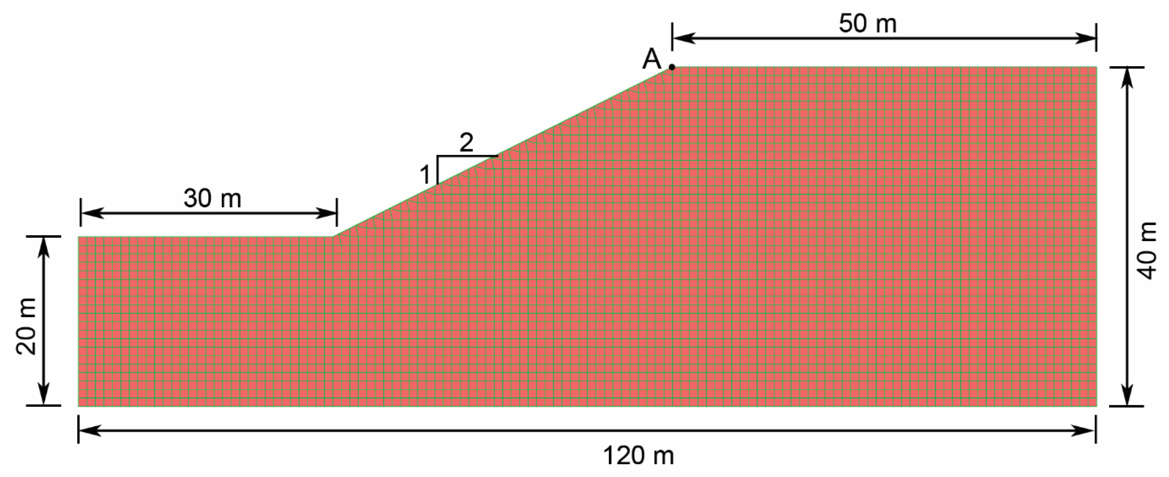
An example of the numerical model discretization of a slope with inclination 2:1 (H:V) using the FLAC program is given in Figure 1. This model is used to examine the effects of the variation of soil properties, the characteristic autocorrelation lengths l_x and l_y, and the intensity and frequency content of the seismic excitation. Two additional numerical models with different slope inclinations are examined later in the paper.

Table 1. Mean value and standard deviation of soil properties.

Property	Mean Value μ	Coefficient of Variation σ/μ
Cohesion c, kPa	30	0.3
Friction angle φ°, degrees	20	0.2
Dilation angle ψ°, degrees	0°	0
Density ρ, kg/m3	2000	0.1
Modulus Ε, MPa	60	0.2
Poisson’s ratio v	0.3	0

gives the mean value $\mu$ and standard variation $\sigma$ of the cohesion c, friction angle φ, Young’s elastic modulus E, and density ρ. The dilation angle ψ and Poisson’s ratio v are also given, but without considering any variation. The cross-correlation coefficients ρ_ij of the properties i and j, based on published experimental data, are given in

Table 2. Correlation coefficients of soil properties.

	$\mathbf{Correlation} \mathbf{Coefficient} {\mathit{\rho }}_{\mathit{i}\mathit{j}}$
Property	c	φ	ρ	E	ν
c	1	−0.5	0.5	0.2	0
φ	−0.5	1	0.5	0.2	0
ρ	0.5	0.5	1	0	0
E	0.2	0.2	0	1	0
ν	0	0	0	0	1

. The ρ_ij values for which no experimental data were found have been considered as equal to zero (Rackwitz, 2000, Zheng Wu, 2013) [20,21].

It should be noted that random fields following the Gauss distribution are defined by their mean value $\mu$, the standard variation $\sigma$, and the autocorrelation function $\rho (x,y)$. The most commonly used expression for the autocorrelation function between two points $\left(x,y\right)$ and $\left(x^{\prime },y^{\prime }\right)$ in a two-dimensional anisotropic space is given by

$$\rho (x,y)=Exp[-\frac{\left|x-x^{\prime }\right|}{l_x}-\frac{\left|y-y^{\prime }\right|}{l_y}]$$

(1)

where $l_x$ and $l_y$ are the characteristic autocorrelation lengths in the horizontal and vertical directions, respectively. These lengths define the scale of fluctuation of the random field. Higher values of autocorrelation lengths indicate a stronger statistical correlation between two points.

Table 3. Autocorrelation lengths.

Autocorrelation Lengths	Cases
	a	b	c
$l_x$, m	20	40	20
$l_y$, m	2	2	4

shows the autocorrelation lengths l_y, l_x in the vertical and horizontal directions, respectively, used in this study (Phoon et al., 1999) [22,23].

To illustrate the development of a numerical model of the slope using random fields of properties, the geometry in Figure 1 is considered. The soil properties are shown in Table 1 and the cross-correlation coefficients are shown in Table 2. The characteristic autocorrelation lengths used are l_y = 2 m in the vertical direction and l_x = 20 m in the horizontal direction. The generation of the random field of the material properties using the LAS method assumes a Gaussian distribution. One realization of the spatial distribution of the random fields of soil cohesion $c$, shear strength angle φ, Young’s modulus $E$, and density ρ is displayed in Figure 2.

The random fields presented in Figure 2 cover a grid of 128 × 64 zones, in which each zone has the dimensions dx = dy = 1 m. It is evident in the random fields in Figure 2 that there are different spatial correlations of the soil properties in the horizontal and vertical directions.

The numerical models developed in this study are subjected to strong ground motion to investigate their seismic performance in terms of permanent displacements at the end of shaking.

Table 4. Historic earthquake records used as excitations.

Earthquake	Mw	R (km)	Recrding	Component	PGA (g)
Kalamata (1986)	6.0	12	Prefecture	Hor.	0.25
Lefkada (2003)	6.4	10	Lefkada	Trans.	0.60
Kobe (1995)	7.2	20	Port Island	Hor.	0.57
Northrdge (1994)	6.7	30	Rinaldi	Hor. 318	0.47
Friuli (1976)	6.5	19	FRiuli	Hor.	0.35

provides the basic characteristics of five historical seismic records used as excitations in the study. These records have been modified to match the acceleration design spectra of Eurocode 8 for rock sites, scaled to a maximum peak ground acceleration of 0.3 g. Figure 3 shows the acceleration response spectra of the modified seismic excitations and the Eurocode 8 acceleration spectra for rock sites.

4. Impact of the Spatial Correlation of Soil Properties

This section examines the impact of the length of spatial correlation on permanent horizontal, vertical, and total displacement. The permanent displacements are evaluated at the top of the slope, indicated as point A in Figure 1.

More specifically, three cases are investigated as shown in Table 3. For case a, the autocorrelation lengths are l_x = 20 m and l_y = 2 m; for case b, they are l_x = 40 m and l_y = 2 m; and for case c, they are l_x = 20 m and l_y = 4 m. All analyses correspond to a sample greater than or equal to 30.

Table 5. Investigation of spatial variability of soil properties (d_x = horizontal length of failure surface and d_y = height of failure surface).

Case Study	lx, m	ly, m	dx m	dy m	lx/dx	ly/dy
1	20	2	90	29.85	0.222	0.067
2	40	2	90	29.85	0.444	0.067
3	20	4	90	29.85	0.222	0.133

shows the data of the cases to be compared. Along with the lengths l_x and l_y, the values of the ratios l_x/d_x and l_y/d_y are also given, where d_x = horizontal length of the failure surface and d_y = height of the failure surface. Figure 4 shows a representative surface of failure and the dimensions d_x and d_y (Alamanis, 2017) [24].

When the lengths l_x and l_y tend to infinity, then the soil becomes homogeneous. Conversely, when the lengths l_x and l_y tend to zero then the soil changes its properties randomly without any correlation between two adjacent or distant points. The use of ratios l_x/d_x and l_y/d_y helps us better understand the impact of spatial variability of soil properties in relation to the dimensions of the expected failure surface. Indeed, when the ratios l_i/d_i take values greater than one or two (l_i/d_i > 1 or 2), then the material at a given point has properties with a strong correlation with those found in other points within the failure surface, and thus tends to approach homogeneity. The method of determining the development of the failure surface of slopes is based on monitoring the equivalent plastic strain increment throughout the analysis. When it increases significantly and abruptly along a surface, this suggests that there is significant movement along this surface and indicates the initiation of a sliding failure.

The evolution of the horizontal and vertical displacement at point A for heterogeneous soil (see Figure 1) is given in Figure 5, with residual values at the end of shaking equal to 0.75 m, respectively.

Figure 6 illustrates the probability density function of the permanent horizontal displacement u_x for the various values of l_x and l_y based on the Weibull distribution. It is observed that for a fixed value of l_y = 2 m, when l_x increases from 20 m to 40 m, there is a very small decrease of the dispersion, as the soil becomes relatively homogeneous. Conversely, for a constant value l_x = 20 m, when l_y increases from 2 m to 4 m, the dispersion increases more significantly (Figure 6). Since the sample is significant (30 analyses), this trend can be interpreted as follows: doubling the autocorrelation length at high values (e.g., from 20 m to 40 m), the effect is low as both of these lengths suggest a large spatial autocorrelation. On the contrary, for a doubling of the autocorrelation length in small values (e.g., from 2 m to 4 m), the effect is significant in that the spatial correlation with short distances is small but increases more intensely with the doubling of the length l_y.

In Figure 7, similar results are presented for the vertical permanent displacement, where the differences between the probability of densities are clearer. The results in Figure 7 indicate that there is some quantitative difference in the effect of the spatial correlation between the horizontal and vertical directions. Indeed, for vertical displacements, the doubling of the autocorrelation length significantly affects the dispersion of the results in both short and larger lengths. Finally, Figure 8 and Figure 9 show the results for the total permanent displacement as well as the probability of exceedance of a certain value of total permanent displacement u* for various values l_x and l_y, based on the Weibull distribution. The results on the effect of the length of the spatial correlation of soil properties presented here are given for only three value pairs of l_x/d_x and l_y/d_y ratios (90 simulations in total) due to space constraints.

5. Effect of Slope Inclination

This section examines the effect of slope inclination on the seismic behaviour of the slopes, adopting as performance criterion the permanent displacement at the end of shaking. More specifically,

Table 6. Geometric characteristics of investigated slopes.

Geometry	Inclination (H:V)	Height, m	Angle
A	2:1	20	27°
B	4:3	30	37°
C	1:1	30	45°

presents three slope profiles (A, B, and C) corresponding to slope inclinations 2:1, 4:3, and 1:1, respectively, which have been investigated in this study. A common set of soil properties was assumed for the three slopes given in

Table 7. Mean value and standard deviation of soil properties.

Property	Mean Value μ	Coefficient of Variation σ/μ
Cohesion c, kPa	50	0.3
Friction angle φ°, degrees	30	0.2
Dilation angle ψ°, degrees	0°	0
Density ρ, kg/m3	2000	0.1
Modulus Ε, MPa	60	0.2
Poisson’s ratio v	0.3	0

, in which the soil strength parameters are higher than those in Table 1 to avoid numerical difficulties in the case of steeper slopes. For the case of homogeneous slopes,

Table 8. Permanent displacements of slopes A, B, and C for homogeneous soil.

Geometry	Inclination (H:V)	FS	${\overline{\mathit{u}}}_{\mathit{x}}$, m	${\overline{\mathit{u}}}_{\mathit{y}}$, m	$\overline{\mathit{u}}$, m
A	2:1	2.58	0.39	0.35	0.53
B	4:3	1.71	0.41	0.47	0.63
C	1:1	1.45	0.76	0.54	0.94

shows the static safety factor FS, the mean horizontal permanent displacement u_x, the mean vertical permanent displacement u_y, and the total permanent displacement u for the modified seismic records in Figure 3, matching the Eurocode 8 spectra (for rock sites) with a peak ground acceleration of 0.30 g.

Figure 10 presents the coefficient f_x = u_x/ū_x of horizontal permanent displacement u_x of the heterogeneous slope normalized with respect to the horizontal permanent displacement ū_x of the homogeneous slope for the three slope inclinations. Additionally, Figure 11 and Figure 12 present the coefficients f_y = u_y/ū_y and f = u/ū of the vertical and total permanent displacement of the heterogeneous slope with respect to the corresponding displacements of the homogeneous slope. As the permanent displacements u_x, u_y, u, ū_x, ū_y, and ū correspond to the same mean soil strength for a given slope, the coefficients f_x = u_x/ū_x, f_y = u_y/ū_y, and f = u/ū mainly express the impact of the spatial variability of soil properties, while the changes of the statistical characteristics of f_x, f_y, and f express the impact of slope inclination. As expected, it is shown by the results that increasing the slope inclination significantly increases the ratios of f_x, f_y, and f. The mean values of f for the 2:1, 4:3, and 1:1 slopes are 1.24, 1.54, and 1.90, respectively. It is observed that for the slopes 2:1 and 4:3, some values of f are less than 1, but for the slope 1:1, all values of f are larger than 1. Finally, Figure 13 plots the probability of exceedance of a given value $f^{*}$ of the coefficient f = u/ū of total permanent displacement for the three slopes (u = total permanent displacement, ū = total permanent displacement of homogeneous slope).

To examine the impact of slope inclination on permanent displacements, it is of interest to utilize the derived statistical distribution of the ratio $f_x=u_x/{\overline{u}}_x$ (or $f_y=u_y/{\overline{u}}_y$) and the results of permanent displacements for homogeneous slopes ${\overline{u}}_x$ (or ${\overline{u}}_y$) given in Table 8, combined with the statistical distribution of normalized displacements expressing the temporal and frequency variability of the seismic excitation. For each slope inclination investigated, the combined effects of the spatial variability of soil properties and earthquake characteristics are expressed by the relations:

$$u_x = {\overline{u}}_x \mathbf{RV} (\mathrm{Normal} \mathrm{Distribution} \left[{\mu }_{f_x},{\sigma }_{f_x}\right]) \times \mathbf{RV} (\mathrm{Uniform} \mathrm{Distribution} \left[r_{\min },r_{\max }\right])$$

(2a)

$$u_y = {\overline{u}}_y \mathbf{RV} (\mathrm{Normal} \mathrm{Distribution} \left[{\mu }_{f_y},{\sigma }_{f_y}\right]) \times \mathbf{RV} (\mathrm{Uniform} \mathrm{Distribution} \left[r_{\min },r_{\max }\right])$$

(2b)

where

$u_x$, $u_y$ = horizontal and vertical permanent displacements of heterogeneous slope

${\overline{u}}_x$, ${\overline{u}}_y$ = horizontal and vertical permanent displacements of homogeneous slope

RV = random variate

${\mu }_{f_x}$,${\mu }_{f_y}$ = mean values of the coefficients f_x, f_y

${\sigma }_{f_x}$,${\sigma }_{f_y}$ = standard variations of the coefficients f_x, f_y

$r_{\min },r_{\max }$ = bounds of uniform distribution

For the slope with inclination 2:1, Figure 14a plots a histogram with the distribution of the computed horizontal permanent displacement derived from a sample of 500 values of $u_x$ using Equation (2a). The distribution of $u_x$ is fitted with the Weibull, Extreme Value, and Gamma distributions. Moreover, Figure 14b,c, plot the computed values of the vertical permanent displacements $u_y$ and total permanent displacements $u$.

Similar results on the distribution of permanent displacements for slope inclination 4:3 are presented in Figure 15, and for slope inclination 1:1 in Figure 16. A comparison of the best fit test parameters for the three statistical distributions in all results presented in Figure 14, Figure 15 and Figure 16 shows that the Weibull distribution clearly provides the best fit for all cases.

To examine the effect of inclination of slopes having the same mean strength, the probability density function of horizontal permanent displacements $u_x$ corresponding to the three slopes are compared in Figure 17a. It is evident from Figure 17a that the effect of slope inclination on $u_x$ is substantial, as both its mean value and variation of the results increase significantly with slope steepness. Indeed, the mean values of $u_x$ are 0.51 m, 0.94 m, and 1.28 m for the 2:1, 4:3, and 1:1 slopes, respectively. (It is noted that the mean values of horizontal permanent displacement ${\overline{u}}_x$ of homogeneous slopes from Table 8 are 0.39, 0.41, and 0.76 m, respectively). Moreover, the corresponding standard deviations are 0.138, 0.304, and 0.344 for the three slopes. Similar conclusions for the effects of inclination of heterogeneous slopes on the vertical permanent displacements $u_y$ and total permanent displacements $u$, are derived from Figure 17b,c, respectively.

Moreover, Figure 18a plots the probability of exceedance of a given value of horizontal permanent displacement u_x for slope inclinations 2:1, 4:3, and 1:1. Similar results for the vertical permanent displacement u_y, and total permanent displacements u are given in Figure 18b,c, respectively.

Finally, it should be noted that the numerical results presented in Figure 14, Figure 15 and Figure 16 correspond to seismic excitations having a peak ground acceleration of $a_{g\max }$ = 0.3 g. To investigate the effect of material nonlinearity of permanent displacements of slopes, similar parametric investigations have been conducted for a wide range of peak ground accelerations from 0.05 g to 0.5 g (Alamanis, 2017) [24]. It has been shown that the seismic permanent displacements of a homogeneous slope (${\overline{u}}_x$, ${\overline{u}}_y$) in equation (2) increase with the magnitude of peak ground acceleration $a_{g\max }$ and can be described with an exponential function of the form.

$${\overline{u}}_i=a_i{\left(a_{g\max }/g\right)}^{b_i}$$

(3)

where $a_i$, $b_i$ are constants (Alamanis, 2017) [24].

6. Conclusions

1. The spatial variability of material properties in earth slopes may have a significant effect on their seismic performance. Accounting for this spatial variability using stochastic methods allows for a better evaluation of the expected permanent displacements of slopes due to strong ground motion, and a better design for mitigation of the expected seismic damage.

2. It has been shown by using statistical analyses that the most suitable distributions for the description of permanent seismic displacements are the Gamma, Extreme Value, and Weibull distributions. Among them, the Weibull distribution provides the best fit of the numerical data.

3. The results show, as far as the impact on spatial correlation length of the soil properties is concerned, that for a doubling of autocorrelation length in large values (e.g., from 20 m to 40 m), the effect on horizontal displacements is low, since both of these lengths indicate great spatial autocorrelation. On the contrary, for doubling of autocorrelation length in small values (e.g., from 2 m to 4 m), the effect is significant in that the spatial correlation with short distances is small but increases more intensely with the doubling of distance. Indeed, for vertical displacements, the doubling of the autocorrelation length significantly affects the dispersion of the results.

4. For slopes with the same material strength, the results of the numerical simulations show that both the mean value and standard deviation of permanent seismic displacement increase substantially when slope inclination increases.

5. The automated procedure of combing the Local Average Subdivision algorithm and the FLAC software through the program Mathematica allowed for the efficient execution of complex, time-consuming Monte Carlo simulations and significantly helped the investigation of the effects of the spatial variability of soil properties on seismic permanent displacements.