Abstract
The use of data in the construction industry is growing rapidly. However, projects that do not have multiple stages, such as pile foundation and cantilever wall construction, are difficult to reinforce based on the data of observation. It cannot be said that the design–build construction process is optimized by piling data and active learning. In this paper, a new data-driven framework is proposed so that it can be used even for construction under single-stage conditions. The proposed method adopts a lower safety factor (SF) in the preliminary design than that in the conventional methods, and checks the performance after the building using piling data. Countermeasures are conducted to satisfy the target reliability, if necessary. Focusing on the expected total cost, the parametric studies reveal that the proposed method can reduce the expected total cost under specific conditions, such as lower countermeasure cost, higher failure cost, and higher relative costs of safety measures. Furthermore, our method exhibits robustness, as even with low initial safety factors, the expected total cost does not become excessively larger compared to the conventional methods. The findings highlight the potential benefits of piling data for optimizing construction projects under single-stage conditions.
1. Introduction
Information and communication technology (ICT) are actively used in construction [1,2], and the characterization of geotechnical data and the facilitation of site-specific data are considered important [3]. In addition to enabling us to respond in real-time [4], the measurement equipment on a construction machine also has the potential to improve the reliability of the structures [5,6]. In the field of piling, the press-in piling method, which is one of the pile penetration methods, can obtain contiguous piling data. This method can not only potentially be used for safety confirmation, but also for the prediction of ground information in real-time [7], as shown in Figure 1. However, while the piling data are collected during piling, it is not yet being fully utilized.
As an active learning method for dealing with construction data, the observational method (OM) was first introduced by Peck [8], and was later supported by many other researchers [9,10,11,12], with its use being accepted by guidelines [13,14,15]. Because the Bayesian model can deal with probabilistic problems, and OM and “Bayesian updating” are easy to use together, these methods can account for uncertainties and update the posterior probability based on observations [16,17,18,19,20]. The OM has advantages in geotechnical structures, which have a large degree of uncertainty compared to artificial materials such as concrete and steel. However, it is said that there are several conditions for its implementation [21,22]: (1) the structure must have considerable uncertainty; (2) the response time and cost for monitoring must be appropriate; (3) the field condition must be observable with some reliability; and (4) the building must consist of multiple stages and be reinforceable after the observations. Condition (1) has been met because geotechnical structures have some large uncertainties [23]. Conditions (2) and (3) can be expected to be met due to improvements in ICT. Thus, only the last condition remains unsolved for conducting the OM.

Figure 1.
Utilization of piling data [24].
Figure 1.
Utilization of piling data [24].

In excavation/embankment, for example, where the OM is actively used, measurements in the early stages of building are used to predict the displacement/settlement and are also applied in the next step (e.g., the cuts and fill stages and the prediction of consolidation durations [9,25]). Conversely, few cases have been reported on pile foundations or embedded cantilever retaining walls (i.e., single excavations), in which it is difficult to use construction data [26]. In this paper, such a condition is referred to as “single stage.” However, is condition (4) always necessary?
The following uses of construction data come to mind: (a) for updating the design for the next step using the construction data (i.e., ordinary OM); (b-1) for assessing the performance of the structure and completing the construction (i.e., construction confirmation); (b-2) for designing cheaper structures in advance, anticipating that the performance of the structure can be verified using the construction data; and (c) for reviewing the maintenance or buying insurance based on the construction data [27]. As projects with rotary press-in piling are often not so large (mainly 20–40 piles [28]), method (a) is not practical for pile foundations to take time away from conducting load tests in order to design, order, and prepare the piles. In method (b-1), the cutting of pre-fabricated piles when the pile stops at a high level is expensive and time-consuming, and the pile length mainly depends on the depth of the bearing layer; therefore, no significant changes can be expected. Method (c) has been reported by [29]; however, to the best of our knowledge, it has not been realized. Thus, it is difficult to apply these methods in both small and in single-stage projects, with the exception of method (b-2).
In this paper, we focus on method (b-2) and propose a piling data-driven framework that adopts a lower safety factor (SF) in the preliminary design than that in conventional methods and reviews the reliability after building using the piling data. Countermeasures (CMs) (i.e., emergency/contingency measures) are conducted to satisfy the target reliability, if necessary.
Our proposed concept may be related to “agile” development, which is one of the software development methods [30]. The agile process can be seen as a reaction to plan-based or traditional methods, and it addresses the challenge of an unpredictable world through continuous design improvement and testing based on rapid feedback and change, aiming for total optimization [31]. The majority of the project of geotechnical construction is clearly divided into steps: investigation, design, building, and maintenance (the waterfall methodology). In the proposed method in this paper, risks are addressed at the building stage to ensure the overall safety.
In this paper, we conduct a feasibility study of the proposed method based on the expected total cost, although we understand that it is difficult to apply the proposed method under the current building codes and regulations. Details of the proposed method are described in Section 2 and the expected total cost is introduced to evaluate the value of the piling data. In Section 3.1, the probability of the countermeasure (CM), as well as the failure, are calculated, and the expected total cost is formulated. In Section 3.2, introducing the cost parameters normalized by the building cost, the excepted total costs are calculated based on the concept of the minimum expected total cost. In Section 4, the effect of the parameters related to costs and uncertainties in regard to the optimal cost is studied. The applicability of the proposed method on pile foundations is discussed in comparison with conventional methods. Finally, Section 5 highlights the advantages and limitations of the proposed method in comparison with the similar concept of agile.
2. Proposed Method
The proposed method adopts a low SF in the preliminary design, and examines each pile in a project based on the capacity estimation from the piling data. If insufficient, countermeasures are taken. This approach is intended to review the quality of all piles during construction and to reduce the overall construction costs.
2.1. Proposed Idea of Observational Construction
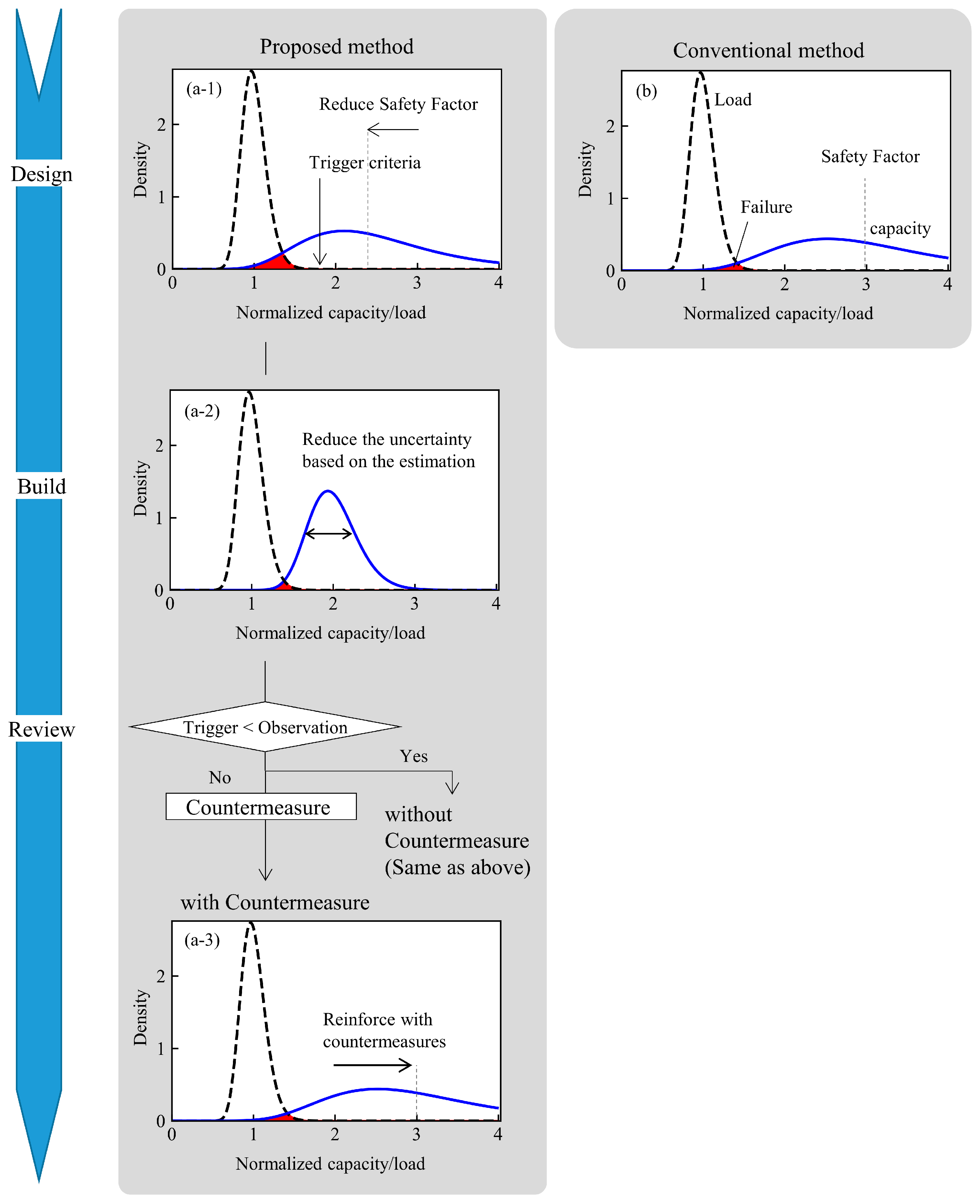
Figure 2 illustrates how the piling data update the probability distribution of the capacity, comparing the proposed and conventional methods.
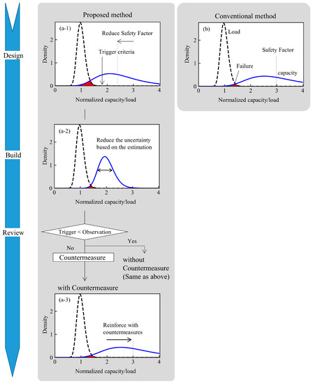
Figure 2.
Imaginary example of the probability distribution. (a-1) probability distributions at the design stage by the proposed method, (a-2) those after building piles, (a-3) those after conducting countermeasures, and (b) those at the design stage by the conventional methods.
To keep the probability of failure in the conventional method under the target value based only on geotechnical surveys, a safety margin (i.e., safety factor) is set, for example, 3.0 (Figure 2b). Failure is defined here as the capacity being lower than the load. However, if a lower SF—for example, 2.4—is applied in the proposed method (Figure 2(a-1)), the probability of failure is naturally larger than the target.
After piling, the capacity is re-estimated using the piling data, and the uncertainty of the estimation is reduced (Figure 2(a-2)). The observation is compared with the trigger criteria (i.e., alert or alarm), which were prepared in advance. When the observed value is less than the trigger criteria, the countermeasure (CM) is implemented in order to ensure the target reliability is obtained (Figure 2(a-3)). The uncertainty after the CM depends on the type of CM. Where the capacity cannot be estimated after the CM, the uncertainty is assumed to be as large as that in the conventional method. This efficiently keeps the final probability of failure in check.
2.2. Flow of the Method
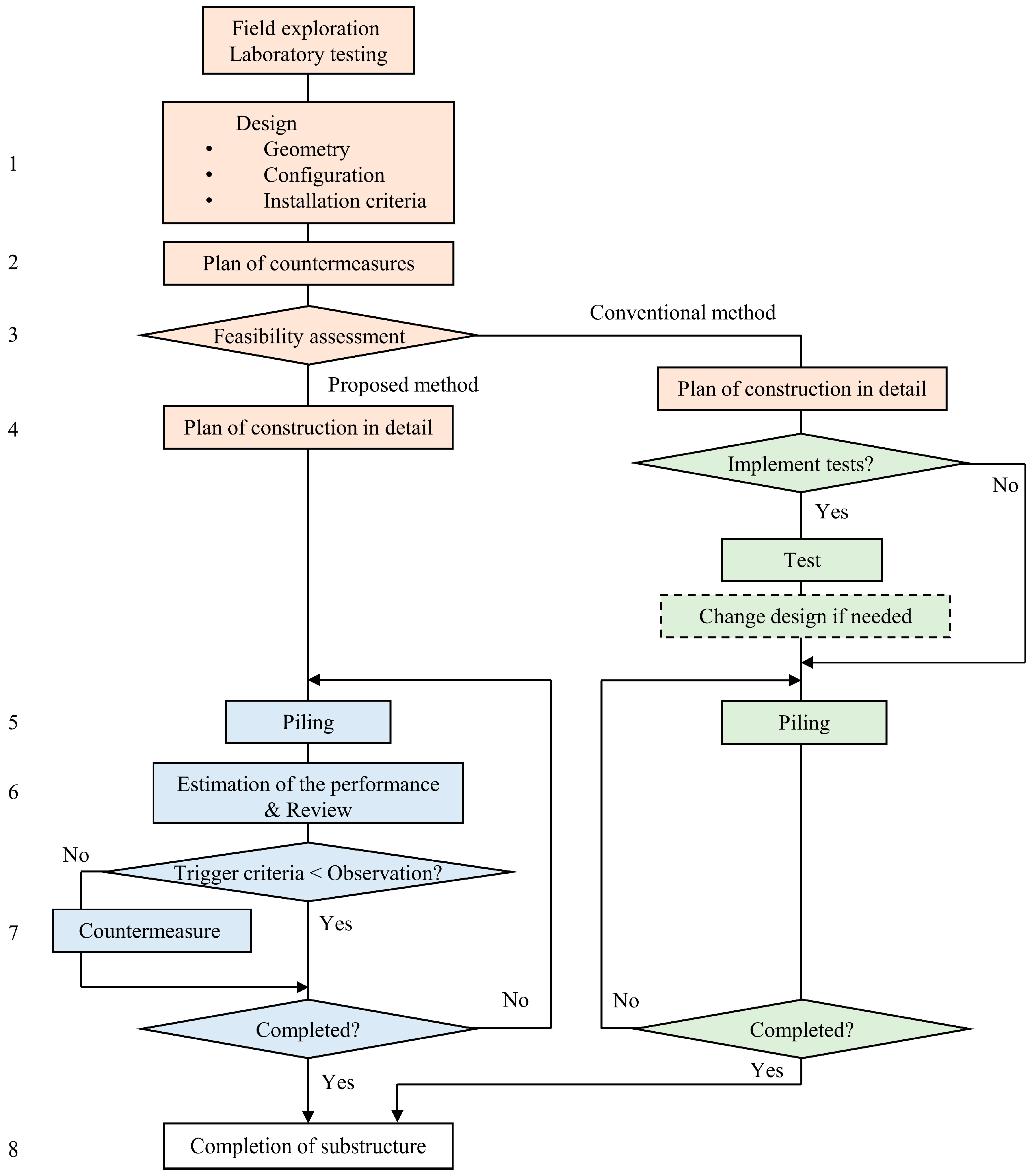
Figure 3 illustrates the flow of the proposed framework, as given below:
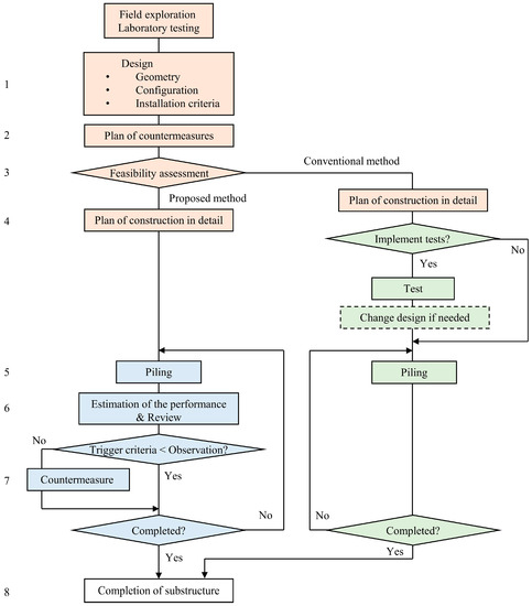
Figure 3.
Flow of the proposed observational construction. The numbers in the figure correspond to the list of numbers in the text.
- Design the preliminary structures based on the investigation.
- Plan candidates of applicable countermeasures from the site conditions, considering the approximate cost.
- Decide if the proposed method is applied based on the expected total cost.
- Plan constructions in detail.
- Build while obtaining piling data.
- Re-estimate the performance and update and review the reliability.
- Take countermeasures if the observed value is less than the trigger criteria.
- Complete the substructure construction if no piles remain.
This ensures reliability despite a low SF.
In the conventional method, when it is difficult to estimate the capacity and the uncertainty of the capacity is larger than usual, on-site tests (e.g., pile load tests) should be conducted, after which the piles are re-designed. The case with load tests is excluded in this paper, assuming that the number of piles is small enough.
2.3. Estimation of Pile Bearing Capacity
Many theoretical and statistical studies have been reported on the bearing capacity of piles. The coefficients of variation (COVs) of cone penetration test (CPT)-based and standard penetration test (SPT)-based estimations of bearing capacity have been reported to be around 30% to 40% [32,33], although it may be larger for unfamiliar soils and pile types.
In piling data based estimations, we estimate the bearing capacity based on the existing formula, such as the dynamic formula for driven piles, empirical formula for vibratory driven piles, and torque-correlation for helical piles (Table 1). Most piling data are measured at the end of the pile installations, and each estimation method is explained in detail in the reference listed in Table 1. Spatial variability is inevitable at the design stage based on the point data obtained from the limited prior ground investigation. However, individual piling data are the in-situ data from the exact same location as the pile foundation. The data and the spatial distribution estimation based on them enable us to reduce or remove spatial variation and to consider only estimation error [34,35]. The COV of the Case Pile Wave Analysis Program (CAPWAP) was reported to be 19%, which included the setup effect [36]. Although the dynamic formula method has less reliability than CAPWAP, there is a strong demand for its use. The COV was reported to be 25% to 28% [37,38]. When the ultimate bearing capacity was estimated by extrapolating the load–settlement curve, the COVs are reported to be 15% when the settlement is 5% of the pile diameter [39].

Table 1.
Typical methods for estimating bearing capacity and required piling data.
Thus, in this paper, the COV in the estimation based on the geotechnical survey (conventional method), COVR;c, is assumed to be 0.35 or 0.50 as representative values, whereas that based on the piling data (proposed method), COVR;p, is assumed to be smaller than 0.25 in anticipation of future technological advances for simply discussing the role of the piling data.
2.4. Type of Countermeasures
There are three types of countermeasures (CMs): extension, addition, and reinforcement. For steel pipe pile foundations and embedded cantilever retaining walls, CMs are extended through the pile length, the number of piles is increased, and the ground around the piles is grouted or the soil in the pipe piles is replaced with concrete. CMs should be selected based on site restrictions and the construction period, considering that extensions are generally the cheapest and reinforcements are the most expensive.
3. Evaluation with Expected Total Costs
The expected total cost, ECtot, is expressed as the sum of the building cost, Cb, countermeasure (CM) cost, Cc, and failure cost, Cf.
where Pc is the probability of CM and Pf is the lifetime probability of failure.
However, it is noted that the formula requires further refinement in reference [44], and we assume that conventional structures have been designed to minimize the expected total cost (Equation (2)).
where subscript T stands for the target value.
The failure cost can be proportional to the building cost, depending on its impact on the economic activity of the site, and the same can be said for the CM cost. Thereafter, for simplicity, we will normalize the costs by the building cost using the parameters, kf and kc; that is, Cf = kf Cb;T and Cc = kc Cb;T.
3.1. Probability Analysis
In this paper, the load, capacity, and estimates of capacity are treated as random variables. By assuming that both the load and capacity follow a lognormal distribution, the probability of failure can be solved analytically, making the calculations of the probability much simpler than running Monte Carlo simulations. Model errors in the estimation of the pile bearing capacity from the geotechnical investigation [45] and piling data [46] were reported to follow log-normal distribution. Meanwhile, the model for the probability distribution of the load depends on the type of load: normal distribution for dead load, lognormal for annual wind load, and Gumbel for wind load [47]. In this study, the dead loads with small variations are basically targeted, although loads with large variations are examined in Section 4.4. The failure probability and reliability index, β, can be calculated analytically [48]:
where COV is the abbreviation for the coefficient of variation, subscripts R and Q represent the capacity and load, respectively, m is the median of the ratio of the capacity to the load, and Φ is the cumulative distribution function (CDF) of the standard normal distribution. Note that the assumption of lognormal distribution may lead to an amplified error of Pf, especially for scenarios with low failure probabilities, and the probability distribution should be determined based on the project condition. The median, mx, and standard deviation, sx, of the lognormal variables are converted from the mean, μx, and standard deviation, σx, as follows:
where subscript X represents variables.
3.1.1. Decision to Implement Countermeasures
The decision to implement CMs is based on whether the reliability index after piling exceeds that of the target.
where subscript ob stands for the value after the observation of the piling data.
All uncertainties (i.e., mean, variance, and probability distribution) are assumed to be known based on detailed database building and analysis, including the estimated variability after obtaining the piling data. As βT is consistent with the value when designing based on geotechnical investigations alone, Pc is calculated as follows:
where we call this characteristic value, mTa, the trigger, and subscripts p and c in the COVR stand for the proposed and conventional methods, respectively.
A smaller COVR;p and larger COVR;c lead to higher triggers and fewer countermeasures. The observed values, mob, follow a lognormal distribution with the median mi and coefficient of variation COVR;c, respectively.
where F() is the normal CDF and subscript i stands for the initial.
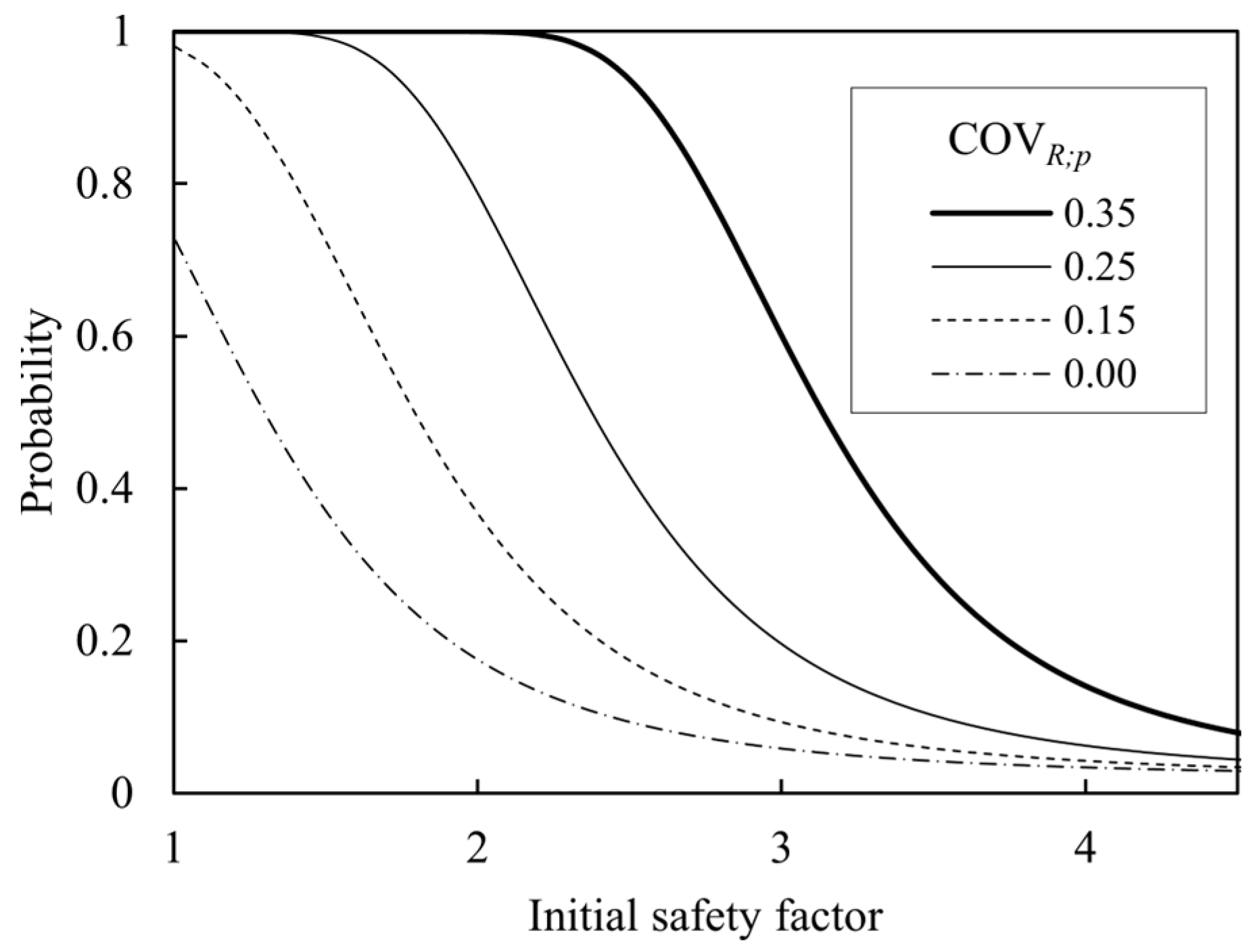
Figure 4 shows the probability of the CM based on Equation (9) when COVR;c = 0.35, COVQ = 0.10, and βT = 3.0, with reference to the findings [32,44,49], respectively. COVR;p = 0.35 requires 60% of the countermeasures even at SF = 3. This is because safety measures were taken due to the misinformation from highly varied estimates. In the paper below, the optimized SF ranges between 2 and 3, wherein it can be observed that the Pc decreases rapidly from a COVR;p of 0.25 to 0.15.

Figure 4.
Example of probability of countermeasure (COVR;c = 0.35, COVQ = 0.10, βT = 3.0). COVR;c and COVR;p are COV of the capacity estimation by the conventional and proposed methods, respectively.
3.1.2. Probability of Failure
The probability of failure, Pf, in the proposed method is expressed as the sum of the conditional probability in the case with the CM and that without the CM. When the CM was conducted, the conditional probability of failure was assumed to be Pf;T. When a higher mob was observed and the CM was not conducted, the conditional probability of failure was re-evaluated with the COVR;p.
where fln() is the lognormal probability density function (PDF), subscript wo stands for without CM, and wi stands for with CM.
Figure 5 shows the Pf based on Equations (10)–(12), assuming that COVR;c = 0.35, COVQ = 0.10, and βT = 3.0. When the initial SF is low, CMs are implemented in most cases, and Pf approaches the target probability, Pf;T (≈10−3). When the initial SF is high, Pf becomes inversely proportional to the initial SF, and is lower than Pf;T. Thus, the proposed method always has a lower probability of failure than the target value.
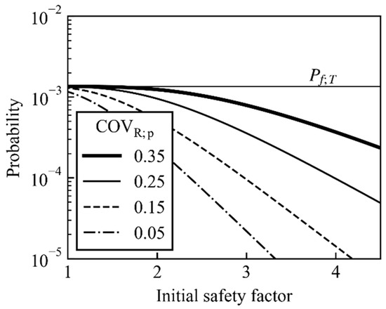
Figure 5.
Probability of failure of the proposed method (COVR;c = 0.35, COVQ = 0.10, βT = 3.0).
3.2. Cost Analysis
In this section, the expected total cost of the proposed method is calculated based on the probability analysis discussed above and the concept of the minimum expected total cost.
3.2.1. Relationship between Building Cost and Initial SF
The building cost is assumed to be a function of the safety factor (SF) in this paper, although some previous research on the minimum expected total cost portrayed the building cost as a function of the reliability index [50,51].
A low SF naturally lowers the building cost; however, the ratio depends on the piling method and has the following three types: the simplest type is that in which the building cost is proportional to the SF [52]; the second type is where a low additional cost is required to increase the SF, or where other costs constitute the majority of the costs, for example, earth-retaining walls or foundations whose superstructures are large; the last type is where a large additional cost is required to increase the SF, for example, where the weight of the structure itself harms the function, or the structure has a bad scale effect. As for open-ended steel pipe piles, the SF is unlikely to be increased by increasing the pile diameter (i.e., cost) because the unit resistance decreases as the pile diameter increases, which is known as the plugging effect [53].
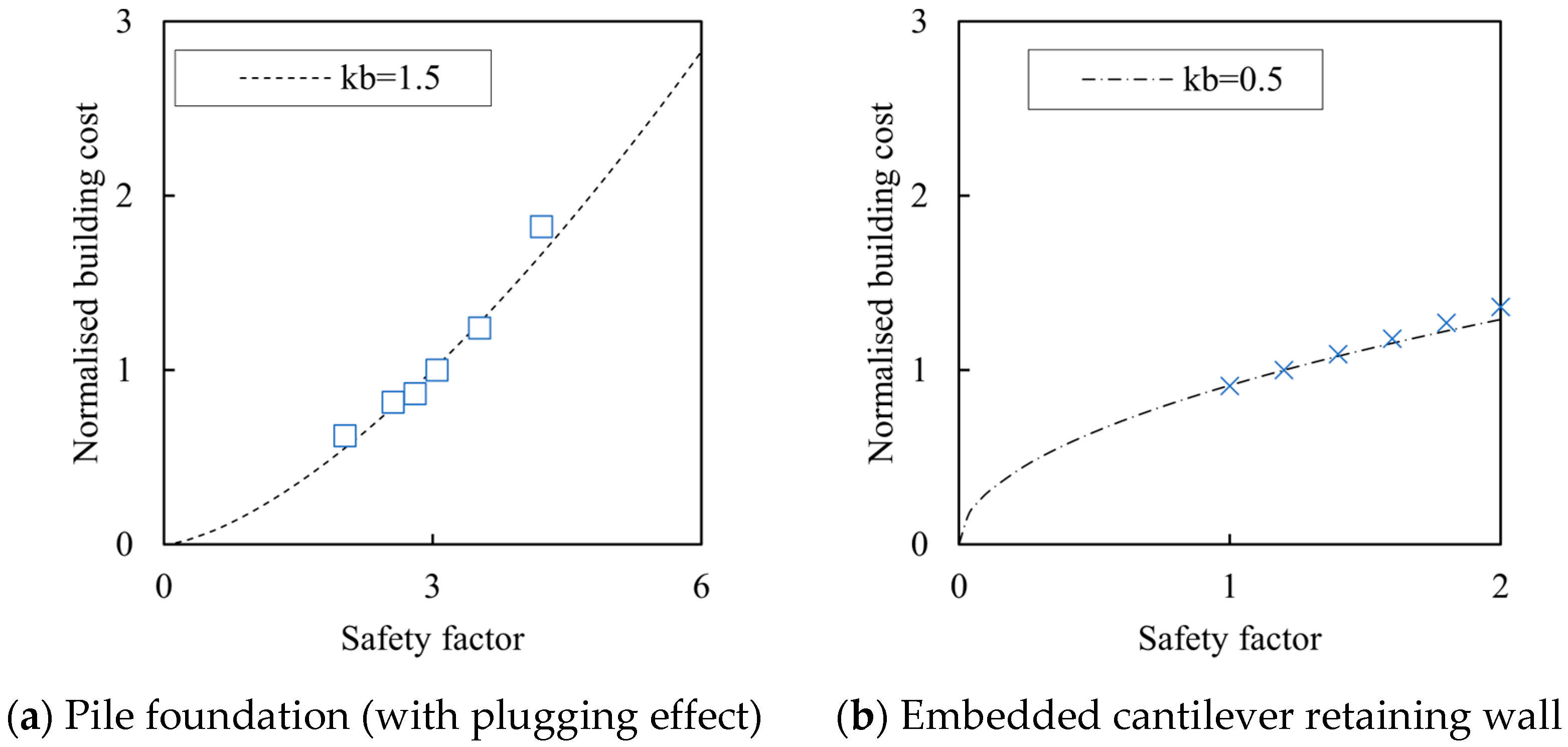
Figure 6 shows examples of cost estimations for open-ended steel pipe pile foundations [54] and steel pipe pile-retaining walls [55]. As the cost estimations conform to the function with the constant power, kb, of the SF (Figure 6), this paper assumes that the normalized Cb is modeled as follows:
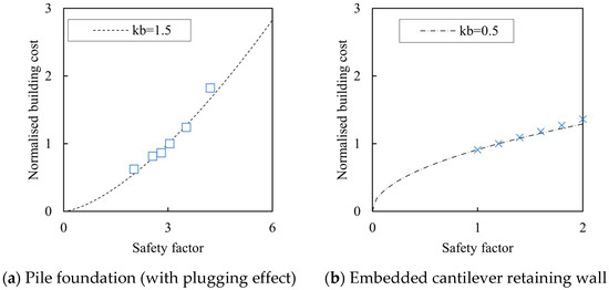
Figure 6.
Relationship between safety factor (SF) and normalized building cost by that of the target one, Cb/Cb;T. The conditions were described by [54,55], respectively.
As kb increases, the incentive to reduce the SF functions better (i.e., relative costs of safety measures noted in [44]. In this paper, kb is assumed to range between 0.5 and 1.5.
3.2.2. Target Reliability Index Based on the Minimum Expected Total Cost
We assume that structures are constructed to minimize the expected total cost [50,56,57]. Although this assumption has sometimes been criticized because of the lack of accuracy in the estimation of the probability of failure and cost, as well as the future change in the demand for performance [58], it is one of the few ways of quantitatively evaluating the safety margins, and is accepted in some guidelines [44,59].
The failure cost varies widely depending on the structure type, location, utility form, evaluation of human life, etc. Kanda and Shah [60] presented losses normalized by the building cost, considering the losses as damage to the structure, function loss, injuries, and fatalities for various building occupation types; the reported normalized losses were 0.1 to 2000. A large kf is used when the structure is important, as in a nuclear power plant, or when the restoration is difficult. However, a value between 0.5 and 2.0 was assumed as kf for port and harbor structures [61], and a value of 10 for pile foundations [52].
Additionally, in the case of no CMs, the expected total cost, ECtot, can be calculated from Equations (1), (3), and (13), as follows:
After substituting Equation (4) for β and differentiating both sides by μ, we obtain:
where f () is the normal probability density function. Substitute 0 for the left side of Equation (15), μT for μ, and βT for β.
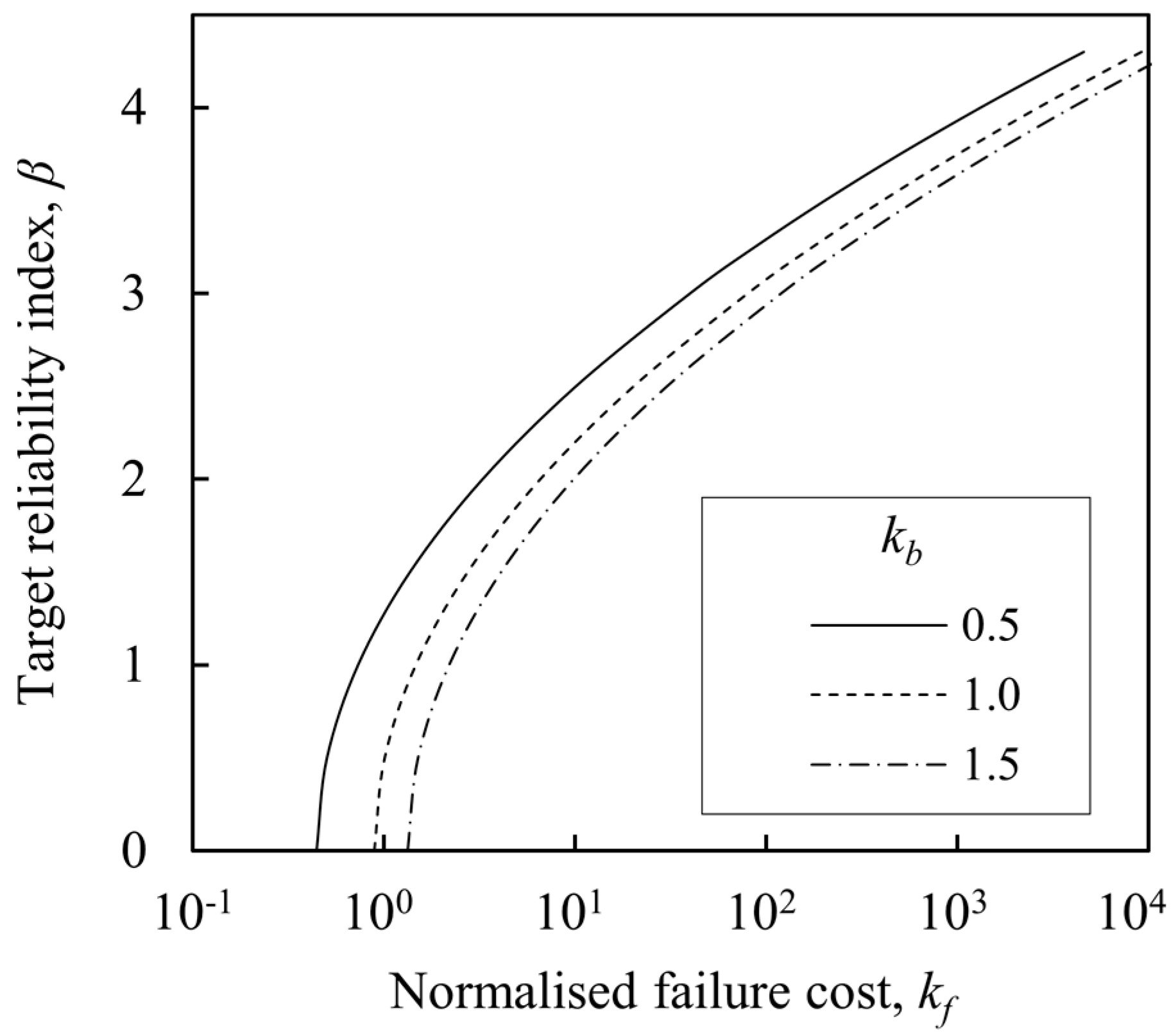
Figure 7 shows the relationship between the normalized failure cost, kf, and β. Equation (16) clearly shows that β is more strongly affected by kf than by kb. If COVR = 0.35, COVQ = 0.10, kb = 1.0, and kf = 80, βT comes to around 3.0. As the range of βT = 0.0–4.3 [44] is roughly consistent with the range of kf indicated by [60], the above assumption seems reasonable.
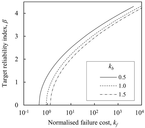
Figure 7.
Relationship between normalized failure cost and target reliability index (COVR = 0.35, COVQ = 0.10).
3.2.3. Ratio of Countermeasure Cost to Building Cost
Although no reports on the countermeasure (CM) cost are available, it is easy to imagine that the cost of reducing the SF and implementing the CMs for all piles is higher than the cost of meeting the target safety.
The CM cost varies widely, depending on the site conditions. By the author’s cost estimation with reference to [62], it is about 1.5 times the building cost when the ground with a width of 50 cm around the steel tubular pile is improved for the entire length of the pile through chemical grouting. Conversely, a simple extension would be cheaper than the piling cost itself. Hence, the parameter related to the CM cost, kc, is temporarily assumed to be in the range of 0.5 to 2.0.
3.2.4. Expected Total Cost
The normalized expected total cost, ECtot, is the function of three vectors based on Equations (1), (9)–(13), and (16):
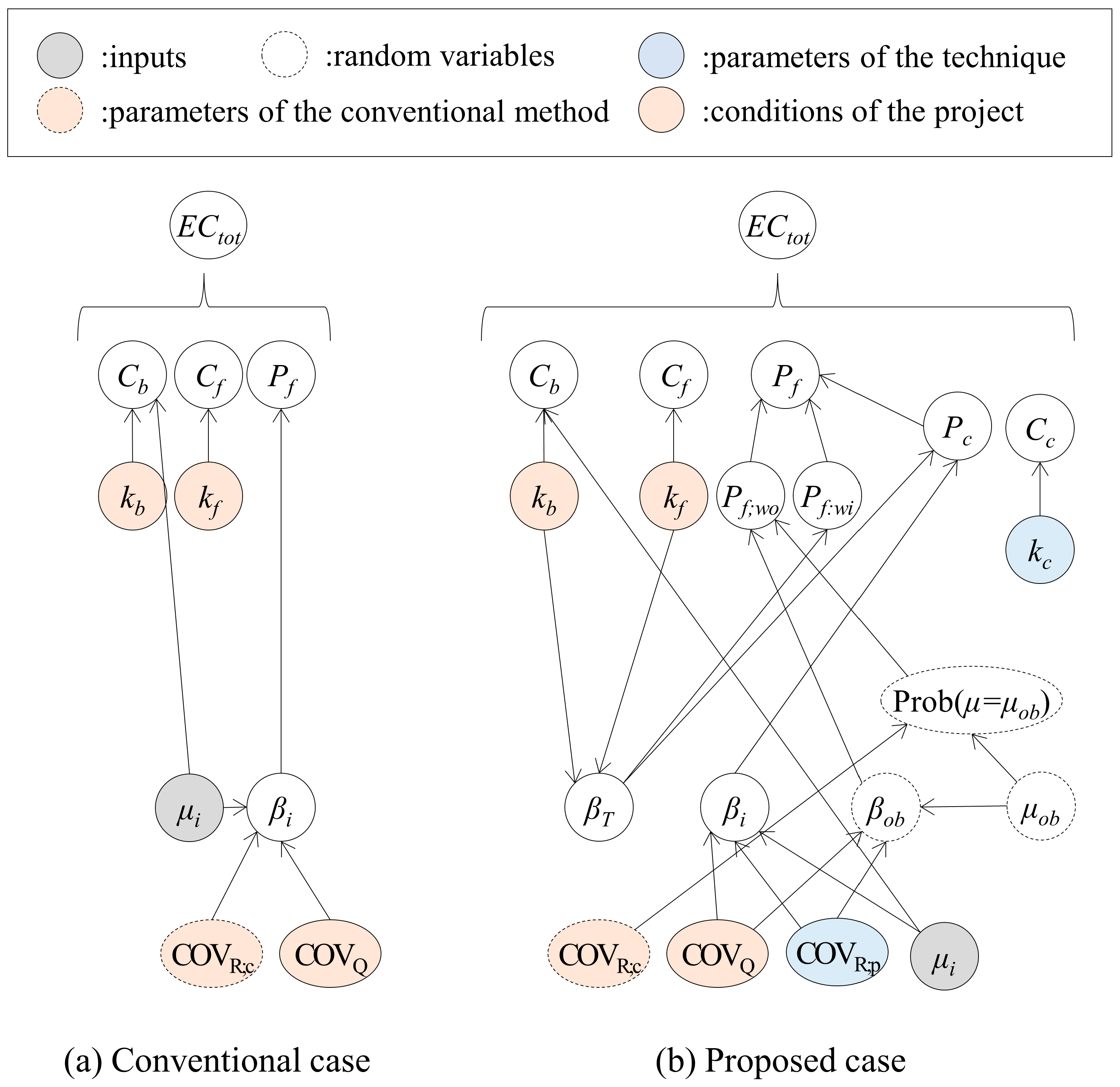
where I is the vector of input {μi}, K is the vector of parameters {kb, kc, kf}, and V is the vector of variability {COVQ, COVR;c, COVR;p}. Figure 8 shows the relationship among the parameters, which differs between the management options—that is, the proposed and conventional cases.
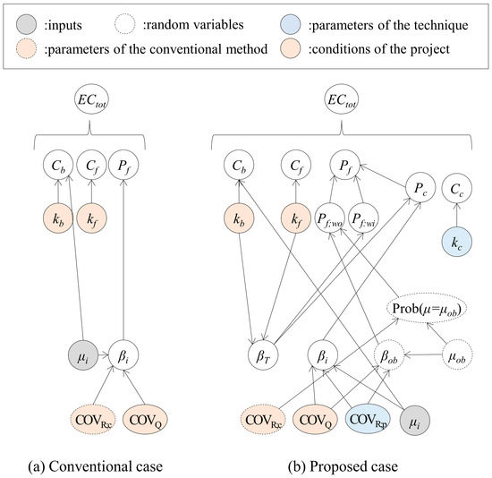
Figure 8.
Graphical models of the parameters for calculating the normalized expected total cost.
The input I is the parameter the designer should select to minimize the expected total cost. Although the optimal value of I is when the derivative of Equation (18) with respect to I is zero, because of the difficulty of differentiation, it is obtained numerically in the next section.
Vectors K and V are divided into three parts in the view of who can change them: conditions of the project {kb, kf, and COVQ}; parameters of the technique {kc and COVR;p}; and parameters of the alternate method {COVR;c}. The conditions of the project depend on the type of project as well as the location, which cannot be changed by contractors and designers. As for the parameters of the technique, makers of the piling techniques may try to reduce the CM cost and increase the reliability of the estimation with the piling data. The parameters of the alternate method will be improved due to new investigation methods [63] or new formulae for estimating the capacity [64].
4. Parametric Studies
This section compares the expected total costs of the proposed method and the conventional method to investigate the applicability of the proposed method and to find the economically optimized design.
Figure 9 describes how the normalized expected costs change with the initial safety factor (SF). In the conventional method, the expected total cost, ECtot, is a downward convex function of the SF and has a minimal value [50]. It is mostly consistent with the building cost with a high SF, while the expected failure cost accounts for most of the expected total cost with a low SF. In this case, the optimized SF becomes 3.0.
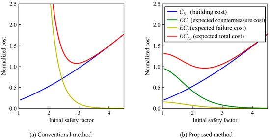
Figure 9.
Constitution of expected total costs (kb = 1.5, kf = 120, kc = 1.0, COVR;p = 0.15).
In the proposed method, ECtot is also a downward convex function of the SF and has a minimal value, as in the conventional method. ECtot is minimized at a SF of about 2.4, which is lower than 3.0 in the conventional case, and even when the initial SF is lower, the expected total cost does not significantly increase, indicating that the proposed method is robust. This is because the countermeasure (CM) cost is significantly lower than the failure cost. Note that when the CM cost is too low, the reduction in the building cost exceeds the increment in the cost of the CMs, and the minimal value does not appear, as noted in Section 3.2.3. This is not realistic, and will be excluded from further consideration.
4.1. Influence of the Parameter Related to Project Condition on the Applicability
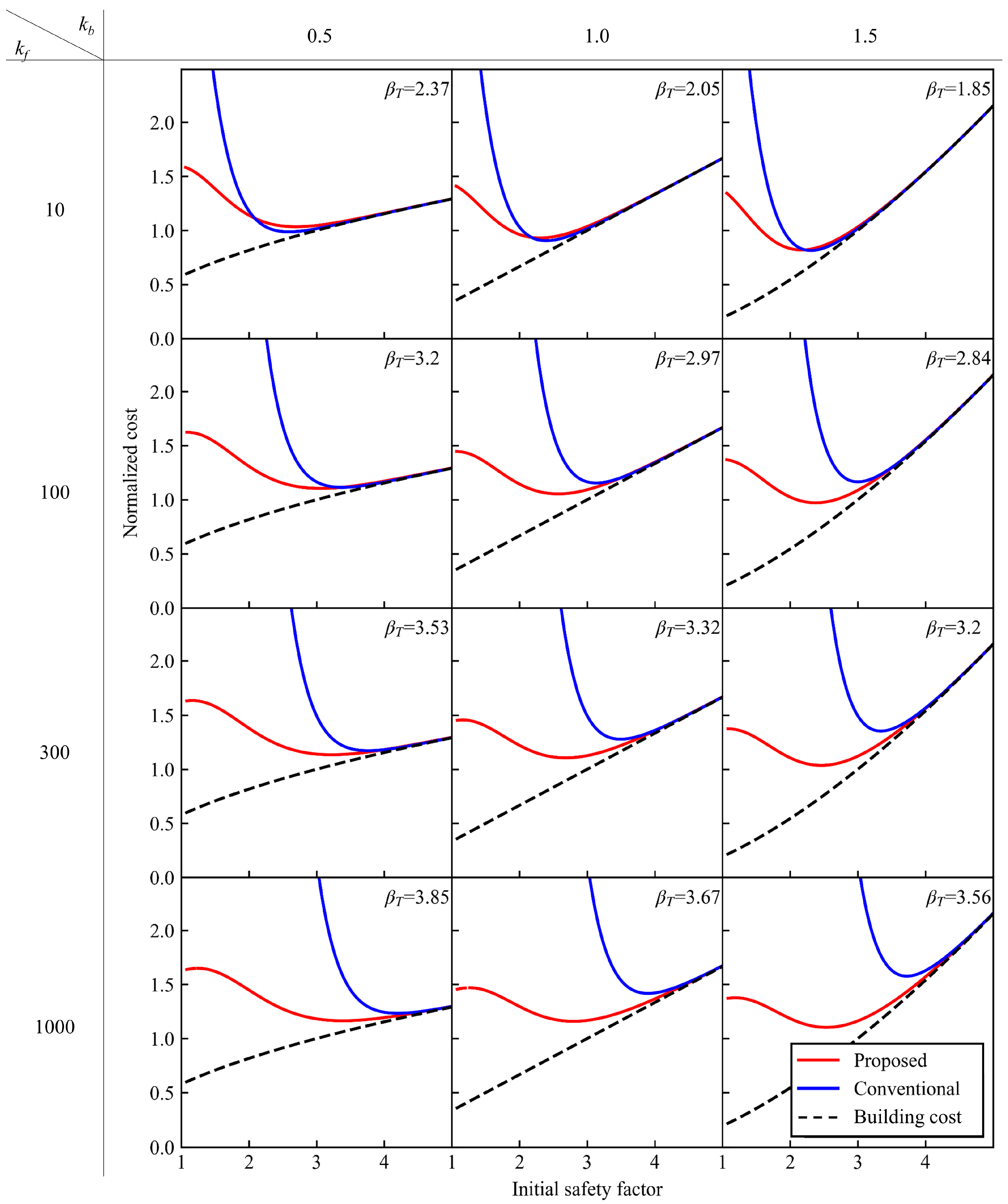
First, check the parameters related to the project condition: kb is related to the building cost and kf to the failure cost. Figure 10 compares the ECtot of both the proposed and conventional methods.
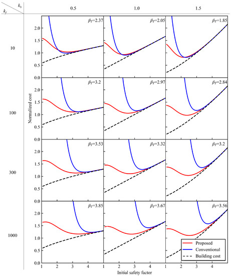
Figure 10.
Influence of kb and kf on expected total costs (COVR;p = 0.15, kc = 1.0). kb and kf are parameters relating to building cost and failure cost, respectively.
In the conventional method, the optimal SF and the optimal ECtot increase with an increase in kf. Additionally, as kb becomes higher, the optimal SF becomes smaller because the incentive to decrease Cb becomes more significant.
In the case of the proposed method, the optimized ECtot seems to change only slightly. This is because ECf is a small part of the ECtot (Figure 9). The optimized ECtot of the proposed method becomes less than that of the conventional method when kb and kf are high; in other words, structures that are easily costly require a high performance and high reliability.
4.2. Influence of the Technique Parameter on the Applicability of the Proposed Method
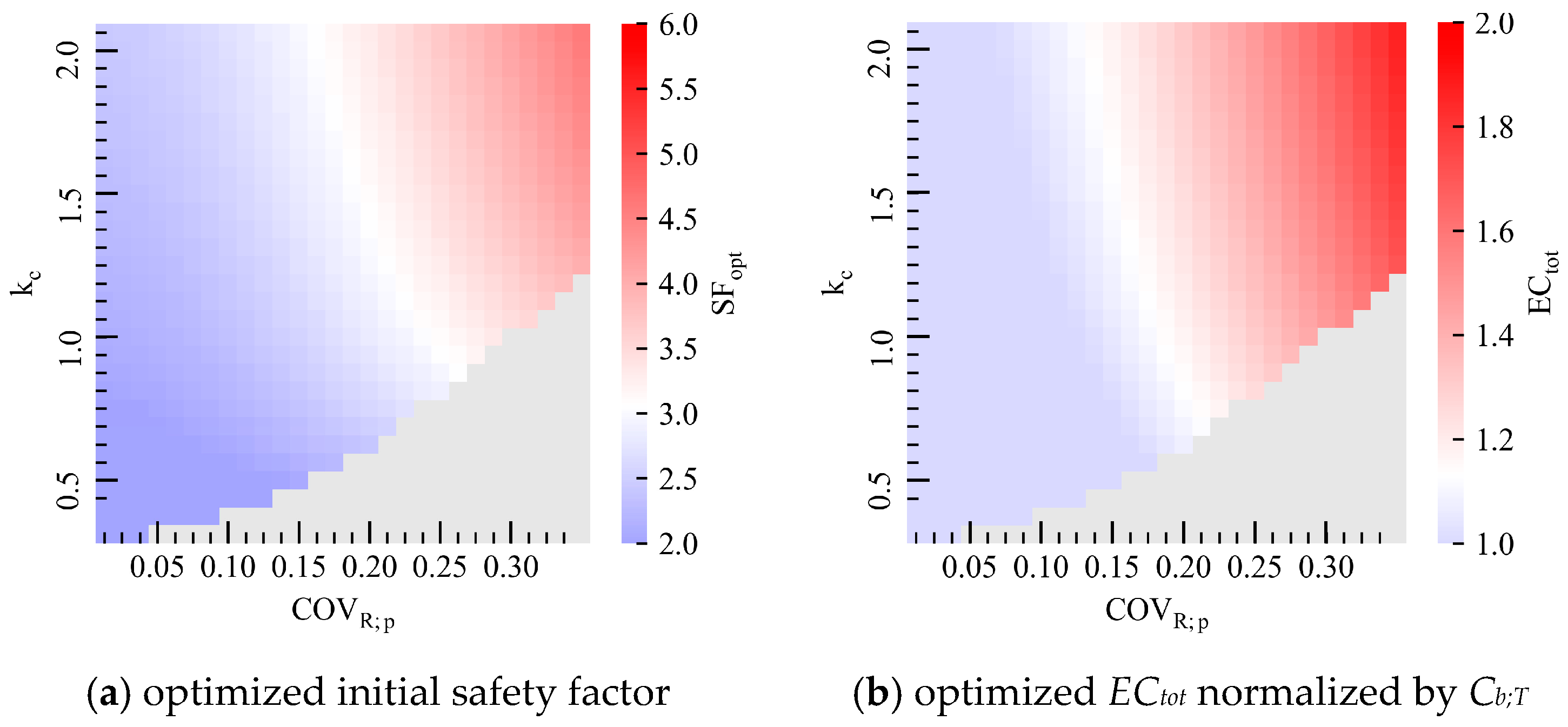
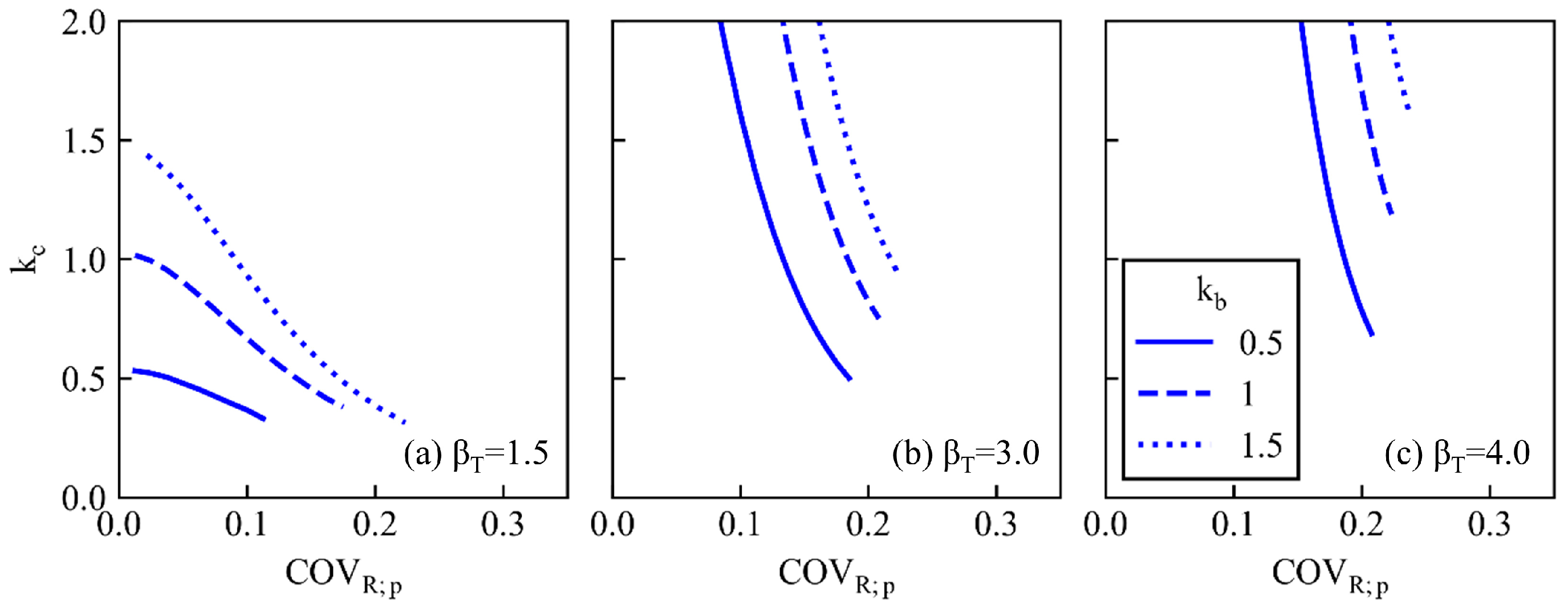
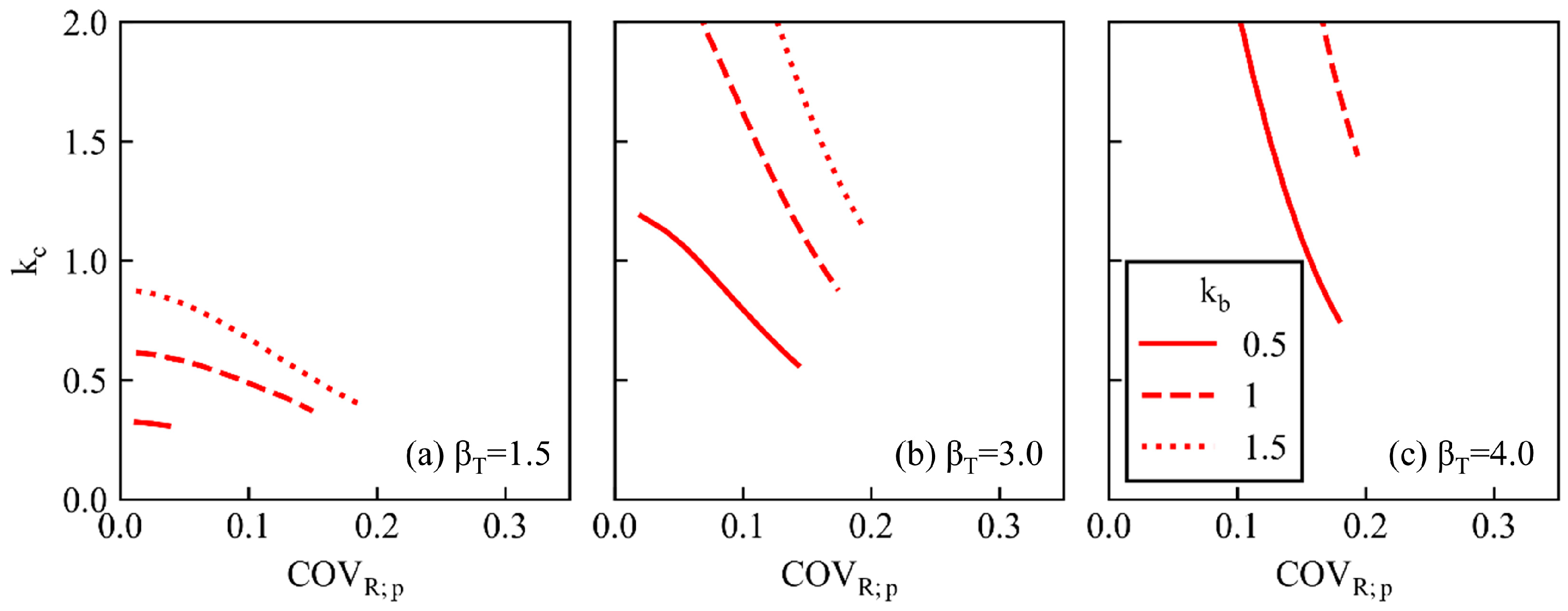
In this paragraph, we analyze the effect of the parameter related to the techniques proposed—that is, kc and COVR;p—on its applicability. Figure 11 shows heatmaps that present the optimized initial SF and ECtot of the proposed method. The heatmaps of the conventional method are drawn in white, which we hereafter call the boundary line, as they are independent of the parameters, kc and COVR;p, and become constant. Note that “optimized” is defined as the point of the minimal cost in each method, as shown in Figure 9.
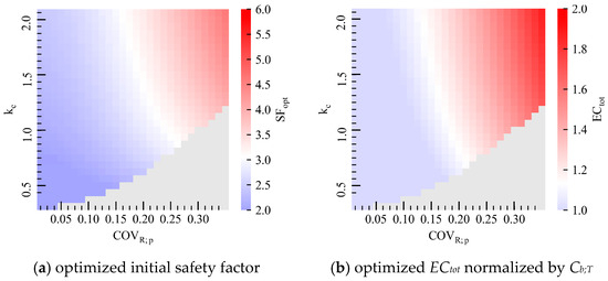
Figure 11.
Relationship between the parameters of the proposed method (COVR;p and kc) and SF and ECtot when kb = 1.0 and kf = 80. The median color of the heatmaps represents the optimum value for the conventional method.
A smaller COVR;p and kc obviously result in both lower optimal SF and ECtot. The boundary line of the ECtot deviates more to the left than that of the SF because the same initial SF results in the additional countermeasure (CM) cost. Even if kc is greater than 1, meaning that the cost of the CM is greater than the target building cost, the proposed method can still be adopted when COVR;p is lower than 0.2. This may seem unnatural at first, but it is because the implementation of CMs is judged based on observations, and as a result, the total cost can be small.
Figure 12 shows the probability of CMs when ECtot is optimized. A higher countermeasure cost (kc) and lower variation in estimation (COVR;p) reduce the countermeasures (lower Pc) and raise the optimized initial SF to avoid additional costs.
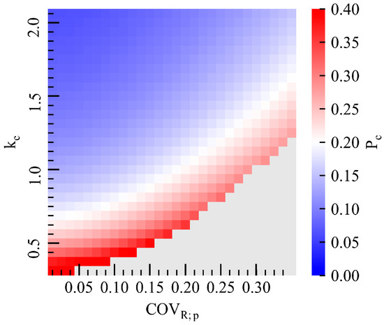
Figure 12.
Relationship between the parameters of the proposed method (COVR;p and kc) and Pc when kb = 1.0 and kf = 80.
The gray area on the lower right of Figure 11 and Figure 12 was excluded because it did not have a minimal value of ECtot (see Figure 9). This is because the expected total cost in the gray area is not a downward convex function and the expected total cost decreases when the SF is too low. To prevent this, the cost of the countermeasure could be a function of the observed value itself, rather than a constant. However, it is difficult to calculate a realistic cost ratio for the preparation and planning of countermeasures, and more specific works need to be considered. We believe that kc = 0.7 is not too large and is realistic enough to consider. Therefore, the gray area is left for future research.
4.3. Influence of βT on the Applicability of the Proposed Method
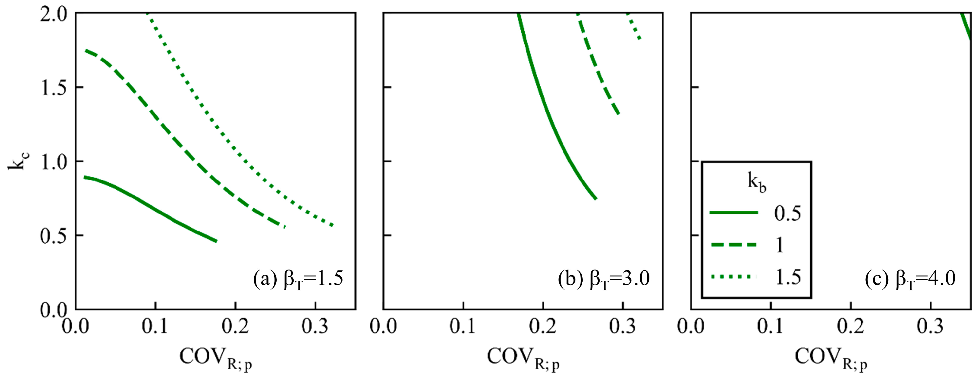
Figure 13 shows the boundary lines, which indicate the case when the conventional and proposed methods have the same expected cost, considering the parameters βT and kb. The lower left area of each boundary line indicates the applicable area of the proposed method. Note that kf differs in each case because it is the function of βT and kb, as shown in Equation (16). The target reliability index, βT, 1.5, 3.0, and 4.0 imply serviceability limit state (SLS), lower level of ultimate limit state (ULS), and higher level of ULS, respectively, with reference to [44].
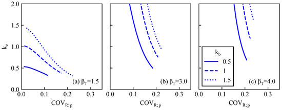
Figure 13.
Applicability of the proposed method (COVQ = 0.10, COVR;c = 0.35). (a) the target reliability index, βT = 1.5, (b) βT = 3.0, and (c) βT = 4.0.
As kb increases, the boundary line moves to the upper right and the applicability widens, which is explained in Figure 10.
The slope of the boundary line changes with βT. When βT is greater than 1.5, the line seems vertical, and the applicability of the proposed method is primarily associated with COVR;p. Conversely, when βT is as small as 1.5, both kc and COVR;p are important. In other words, both the CM costs and the uncertainty of the estimation using piling data need to be reduced. Moreover, even if COVR;p is extremely low, kc must be less than a certain value (Figure 13a).
4.4. Influence of COVQ and COVR;c on the Applicability
For the remaining parameters, a lower COVQ and higher COVR;c naturally expand the applicability of the proposed method.
Loads generally consist of dead loads, impact loads, and seismic loads, and the variability depends on their proportions. Variable loads are typically modeled with the extreme distribution. This has a heavier tail than the lognormal distribution, which would underestimate the probability of failure, especially at a high target reliability index. However, a lognormal distribution was also used for the higher COVQ case to focus on the differences in the amount of variation in this paper.
Figure 14 illustrates the boundary lines when the COVQ increases to 20%. The boundary lines move to the lower left compared to Figure 13. This is because the value of updating the capacity with the piling data would decrease, and consequently, the applicability of the proposed method would also decrease. Note that a distribution with a heavier tail would further limit the applicability of the proposed method.
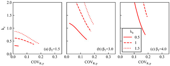
Figure 14.
Influence of other parameters on applicability (COVQ = 0.20, COVR;c = 0.35).
Although the COVR;c was assumed to be 0.35 for soils whose characteristics are well known, it should be larger for unfamiliar rocks with high spatial variability. Figure 15 illustrates the boundary lines if the COVR;c increases to 50% with reference to [65]. The boundary lines move to the upper right, contrary to those in Figure 14, and the applicability of the proposed method increases significantly. When βT is 4.0, the visible area in Figure 15c can be mostly applied to the proposed method.
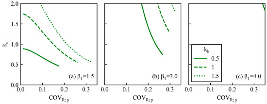
Figure 15.
Influence of other parameters on applicability (COVQ = 0.10, COVR;c = 0.50).
Hence, the proposed method seems less effective in cases in which seismic loads are dominant in determining the structural parameters or in cases in which the reliability of the design using the conventional method improves. Conversely, the scope of the application of the method increases when dead loads are dominant or when the information about the ground and piling methods is insufficient.
5. Discussions
5.1. Advantages of the Method Proposed
Based on the above-mentioned parametric studies, the proposed method is more cost-beneficial than the conventional method in the cases listed below. The parameters are categorized in Figure 7 and the conditions referred to in the Introduction were also noted for reference.
- (A)
- Parameters of the technique
- Low cost of countermeasure (kc), which was the same as Condition (2)
- Low uncertainty of estimation of the proposed method (COVR;p), which was the same as Condition (3)
- (B)
- Parameters of the conventional method
- High uncertainty of estimation of the conventional method (COVR;c), which was the same as Condition (1)
- (C)
- Conditions of the project
- High failure cost (kf)
- Where the structure requires high reliability (βT)
- When the building cost tends to increase with an increase in the SF (kb)
- Low uncertainty of loads (COVQ)
- Small scale of the projects
The conditions required for the OM listed in the Introduction are all included in (A) and (B). Makers of piling techniques can develop and improve the piling technique through flexible responses to differences between the design and observed results, the development of efficient countermeasure methods, and the development and improvement of the estimation methods. Which of these should be prioritized depends on the performance requirements, as stated previously.
The remaining condition is (C), under which, at first glance, it may seem unusual to decrease the initial SF where the failure cost is large and the structure requires high reliability. However, this is understandable when considering that the conventional method requires a larger SF, whereas the proposed method does not.
A larger reliability index is better for the proposed method. Initially, it appears that the ULS should be dominant in determining the design parameters. However, this assumes that the COVR;p and COVR;c remain the same, which they generally do not. The estimated variation in deformation is higher than that of the ultimate capacity. Furthermore, the measured deformation during piling could be the initial elastic deformation. Therefore, the COVR;c is expected to be higher and the COVR;p and kf lower for SLS than for ULS. Hence, it cannot be determined in this paper whether piling data are more important for the ULS or SLS.
As variations in the loads cannot be handled during construction, it is naturally appropriate that they are smaller; that is, the dead load should be dominant instead of the live load.
If the project size and number of piles are large, there will be more time to conduct preliminary geotechnical investigations and loading tests. In such cases, the estimated variation COVR;c will be smaller and the likelihood of adopting the proposed method will be lower. The relationship between the number of piles and the cost of conducting loading tests was nomogrammed by [66], showing that around 50 piles would be the threshold to determine whether load tests should be undertaken for the project.
Assuming that kc is 1.0 at most by simply adding new piles, kb is greater than 1.0 and βT is more than 3.0, the proposed method seems highly applicable (Figure 13). To make the proposed method more applicable for the ULS, reducing the COVR;p takes priority over reducing the kc.
5.2. Limitations of the Method Proposed
The proposed method has certain limitations, some of which are common to the agile method described in the Introduction, while others are due to the differences between software development and construction projects.
Similar to agile development [31], the proposed method faces the following challenges: (1) difficulty in predicting the construction period in advance; (2) dependence on experienced teams with knowledge of both design and construction; (3) suitability for small teams; (4) lack of comprehensive documentation that prevents accountability, as the proposed method may not provide clear estimation in advance. Many of these also apply to the ordinary observational method, the limitations and critiques of which have been discussed by [22,67,68]. Other limitations also exist, including difficulty in preventing data falsification and deciding the responsibility for the risks.
As for what is unique about hardware development, the cost of production is higher. It takes a lot of time to erase something once it is created, and it is difficult to ensure that the completed structure adequately meets the requirements. This tendency is more pronounced in single-item production at the site, where extra work such as countermeasures tends to be avoided. On the other hand, if the construction and data are divisible and can be updated for each part, as in the proposed method, the CM cost is not so high and is not critical.
5.3. Comparison with Other Alternatives for Maintaining the Reliability of Geotechnical Structures
To ensure a certain level of reliability for geotechnical structures, there are options at each of the following stages: investigation, building, inspection, and management. If the project size is large, it should be thoroughly investigated before the building stage. If the speed of the project is important, the minimum amount of investigation is required, and the construction data will ensure the reliability of the structure. If complicated management is not desired, the construction can be carried out with a high SF, or if it is easy to modify the structure after inspection and maintenance, that is also an option.
As embedded geotechnical structures are difficult to inspect and repair after building, detailed geotechnical investigations are usually required in advance. The proposed method increases the flexibility of project management. It will be effective when detailed geotechnical investigations are difficult due to the surrounding site conditions, or when the project duration needs to be shortened. The method increases the value of the piling data, and the observation and use of data during building increase due to improvements in the measuring instruments and data sharing methods. Finally, further discussions on management methods such as those described in this paper are required.
6. Conclusions
In this paper, a piling data-driven framework is proposed for single-stage building such as excavation for cantilever retaining walls and pile foundations. The proposed method applies a low safety factor in the preliminary design and reviews the reliability based on the piling data. Countermeasures are taken if the reliability index is greater than the target.
To analyze the applicability of the proposed method, the expected total cost was compared with the conventional method, and the following conclusion can be drawn under some assumptions:
- The expected total cost is a function of three vectors: ones for cost parameters, ones for uncertainties, and inputs such as the initial safety factor.
- The expected total cost of the proposed method is a downward convex function of the safety factor and has a minimum value similar to that of the conventional method. The proposed method is a robust design, as the expected total cost does not become extremely large compared to the conventional methods, even when the initial SF is low.
- The proposed method can reduce the expected total cost on the following conditions: low cost of countermeasure (kc); low uncertainty of estimation of the proposed method (COVR;p); high uncertainty of estimation of the conventional method (COVR;c); high failure cost (kf); when building costs tend to increase for the increasing safety factor (kb); where the structure requires high reliability (βT); low uncertainty of loads (COVQ), such as when the dead load is dominant; and the small scale of the projects.
- Makers of piling techniques can reduce two parameters to expand the applicability of the proposed method: the cost of the countermeasure and the uncertainty of the re-estimation. Reducing the uncertainty in estimating the bearing capacity using piling data (COVR;p) has priority over reducing the countermeasure cost (kc) for the ultimate limit state. Conversely, when high reliability is not required, it is important to reduce both.
- The limitations of the proposed method include challenges similar to agile development, such as the difficulty in predicting construction timelines and the need for experienced teams. Comparatively, the method increases project management flexibility and the value of the piling data, but requires further discussions of the management methods and adequate cases depending on the project size and requirements under the current regulations.
Author Contributions
Conceptualization, N.S.; methodology, N.S. and K.N.; formal analysis, N.S.; investigation, N.S.; writing—original draft preparation, N.S.; writing—review and editing, K.N.; visualization, N.S. All authors have read and agreed to the published version of the manuscript.
Funding
This research received no external funding.
Institutional Review Board Statement
Not applicable.
Informed Consent Statement
Not applicable.
Data Availability Statement
The data that support the findings of this study are available from the corresponding author upon reasonable request.
Conflicts of Interest
The authors declare no conflict of interest.
Nomenclature
| Cb | building cost |
| Cb;T | Cb to obtain more than target probability of failure by conventional method |
| Cc | cost of countermeasure |
| Cf | cost of failure |
| ECtot | expected total cost |
| fln | lognormal probability function |
| Fln | cumulative lognormal probability function |
| kc | parameter of countermeasure cost |
| kf | parameter of failure cost |
| kb | parameter of piling cost |
| m | median |
| Pc | probability that countermeasures will be required |
| Pf | lifetime probability of failure |
| Pf;T | target probability of failure |
| Pf;wi | conditional probability of failure with countermeasure |
| Pf;wo | conditional probability of failure without countermeasure |
| s | standard deviation of lognormal variable |
| a | parameter to indicate trigger criteria |
| β | reliability index |
| βi | initial reliability index at design stage |
| βT | target reliability index |
| βob | reliability index after evaluation with observational data |
| μ | average |
| σ2 | variance |
| COV | coefficient of variation |
| COVR;c | COV of the capacity estimation by conventional method |
| COVR;p | COV of the capacity estimation by proposed method |
| COVQ | COV of the load |
| SF | safety factor |
| OM | observational method |
| CM | countermeasure |
References
- Adriaanse, A.; Voordijk, H.; Dewulf, G. The Use of Interorganisational ICT in United States Construction Projects. Autom. Constr. 2010, 19, 73–83. [Google Scholar] [CrossRef]
- Cepa, J.J.; Pavón, R.M.; Alberti, M.G.; Ciccone, A.; Asprone, D. A Review on the Implementation of the BIM Methodology in the Operation Maintenance and Transport Infrastructure. Appl. Sci. 2023, 13, 3176. [Google Scholar] [CrossRef]
- Ching, J.; Phoon, K.-K. Modeling Multivariate, Uncertain, Sparse, and Incomplete Site Investigation Data with Spatial Variation (MUSIC-X). In Proceedings of the 7th International Symposium on Geotechnical Safety and Risk (ISGSR 2019), Taipei, Taiwan, 11–13 December 2019; pp. 334–339. [Google Scholar]
- Omar, T.; Nehdi, M.L. Data Acquisition Technologies for Construction Progress Tracking. Autom. Constr. 2016, 70, 143–155. [Google Scholar] [CrossRef]
- White, D.J.; Vennapusa, P.K.R.; Zhang, J.; Gieselman, H.; Morris, M. Implementation of Intelligent Compaction Performance Based Specifications in Minnesota; Mn/Rc 2009-14; Minnesota Department of Transportation: St. Paul, MN, USA, 2009; 337p.
- Hu, M.; Li, W.; Yan, K.; Ji, Z.; Hu, H. Modern Machine Learning Techniques for Univariate Tunnel Settlement Forecasting: A Comparative Study. Math. Probl. Eng. 2019, 2019, 7057612. [Google Scholar] [CrossRef]
- Ishihara, Y.; Haigh, S.; Bolton, M. Estimating Base Resistance and N Value in Rotary Press-In. Soils Found. 2015, 55, 788–797. [Google Scholar] [CrossRef]
- Peck, R.B. Advantages and Limitations of the Observational Method in Applied Soil Mechanics. Géotechnique 1969, 19, 171–187. [Google Scholar] [CrossRef]
- Asaoka, A. Observational Procedure of Settlement Prediction. Soils Found. 1978, 18, 87–101. [Google Scholar] [CrossRef]
- Powderham, A.J. An Overview of the Observational Method: Development in Cut and Cover and Bored Tunnelling Projects. Géotechnique 1994, 44, 619–636. [Google Scholar] [CrossRef]
- Yeow, H.C.; Nicholson, D.; Man, C.L.; Ringer, A.; Glass, P.; Black, M. Application of Observational Method at Crossrail Tottenham Court Road Station, UK. Proc. Inst. Civ. Eng. Geotech. Eng. 2014, 167, 182–193. [Google Scholar] [CrossRef]
- Powderham, A.; O’Brien, T. The Observational Method in Civil Engineering: Minimising Risk, Maximising Economy, 1st ed.; CRC Press: London, UK, 2020; ISBN 9780429344244. [Google Scholar]
- Nicholson, D.; Tse, C.; Penny, C. The Observational Method in Ground Engineering Principles and Applications (C185); CIRIA: London, UK, 1999; ISBN 978-0-86017-497-4. [Google Scholar]
- EN 1997-1; Eurocode 7: Geotechnical Design—Part 1: General Rules. European Committee for Standardization: Brussels, Belgium, 2004.
- Gaba, A.R.; Hardy, S.; Doughty, L.; Powrie, W.; Selemetas, D. Guidance on Embedded Retaining Wall Design (C760); CIRIA: London, UK, 2017; ISBN 978-0-86017-764-7. [Google Scholar]
- Olsson, L.; Stille, H. Observation Systems with Alarm Thresholds and Their Use in Designing Underground Facilities; Swedish Nuclear Fuel and Waste Management Co.: Stockholm, Sweden, 2002. [Google Scholar]
- Straub, D.; Papaioannou, I. Bayesian Updating with Structural Reliability Methods. J. Eng. Mech. 2015, 141, 04014134. [Google Scholar] [CrossRef]
- Spross, J.; Johansson, F. When Is the Observational Method in Geotechnical Engineering Favourable? Struct. Saf. 2017, 66, 17–26. [Google Scholar] [CrossRef]
- Papakonstantinou, K.G.; Andriotis, C.P.; Gao, H.; Chatzi, E.N. Quantifying the Value of Structural Monitoring for Decision Making. In Proceedings of the 13th International Conference on Applications of Statistics and Probability in Civil Engineering, ICASP 2019, Seoul, Republic of Korea, 26–30 May 2019. [Google Scholar]
- Baynes, F.J.; Parry, S.; Novotný, J. Engineering Geological Models, Projects and Geotechnical Risk. Q. J. Eng. Geol. Hydrogeol. 2020, 54, qjegh2020-080. [Google Scholar] [CrossRef]
- Van Baars, S.; Vrijling, J.K. Geotechnical Applications and Conditions of the Observational Method. Heron 2005, 50, 155–172. [Google Scholar]
- Korff, M.; Jong De, E.; Bles, T.J. SWOT Analysis Observational Method Applications. In Proceedings of the 18th International Conference on Soil Mechanics and Geotechnical Engineering: Challenges and Innovations in Geotechnics, ICSMGE 2013, Paris, France, 2–6 September 2013; Volume 3, pp. 1883–1887. [Google Scholar]
- Phoon, K.K.; Tang, C. Characterisation of Geotechnical Model Uncertainty. Georisk 2019, 13, 101–130. [Google Scholar] [CrossRef]
- Ishihara, Y.; Yasuoka, H. Utilization of Monitoring Data during Press-in Piling. In A Brief Development History of Press-In Machinery; International Press-in Association (IPA), Ed.; IPA: Tokyo, Japan, 2022; pp. 31–48. ISBN 9784909722546. [Google Scholar]
- Young, D.K.; Ho, E.W.L. The Observational Approach to Design of a Sheet-Piled Retaining Wall. Geotechnique 1994, 44, 637–654. [Google Scholar] [CrossRef]
- Iwasaki, Y.; Fukuda, M.; Watanabe, H.; Hirata, A.; Hori, Y. Construction Control for Underpinning Piles and Their Behaviour during Excavation. Geotechnique 1994, 44, 681–689. [Google Scholar] [CrossRef]
- ISO 31000:2018; Risk Management—Guidelines. International Organization for Standard (ISO): Geneva, Switzerland, 2018.
- Suzuki, N.; Kimura, Y. Summary of Case Histories of Retaining Wall Installed by Rotary Cutting Press-in Method. In Proceedings of the Second International Conference on Press-In Engineering 2021, Kochi, Japan, 19–20 June 2021; pp. 581–587. [Google Scholar]
- Oyado, M.; Ken, W.; Hidetoshi, N. Survey and Consideration on the Use of Insurance for Risk Management of Civil Structures. In Proceedings of the 74th Annual Conference of the Japan Society of Civil Engineers, Takamatsu, Japan, 3–5 September 2019; Volume 74, pp. IV_291–IV_292. (In Japanese). [Google Scholar]
- Beck, K.; Beedle, M.; Van Bennekum, A.; Cockburn, A.; Cunningham, W.; Fowler, M.; Grenning, J.; Highsmith, J.; Hunt, A.; Jeffries, R.; et al. Manifesto for Agile Software Development. Available online: http://agilemanifesto.org/ (accessed on 1 January 2022).
- Dybå, T.; Dingsøyr, T. Empirical Studies of Agile Software Development: A Systematic Review. Inf. Softw. Technol. 2008, 50, 833–859. [Google Scholar] [CrossRef]
- Yang, Z.; Jardine, R.; Guo, W.; Chow, F. A Comprehensive Database of Tests on Axially Loaded Piles Driven in Sand; Academic Press: Cambridge, MA, USA, 2015; ISBN 9780128047484. [Google Scholar]
- Nanazawa, T.; Kouno, T.; Sakashita, G.; Oshiro, K. Development of Partial Factor Design Method on Bearing Capacity of Pile Foundations for Japanese Specifications for Highway Bridges. Georisk Assess. Manag. Risk Eng. Syst. Geohazards 2019, 13, 166–175. [Google Scholar] [CrossRef]
- Tomizawa, Y.; Yoshida, I.; Otake, Y. Spatial Distribution Estimation Considering Correlation among Multiple Geotechnical Properties Using Gaussian Process Regression. Artif. Intell. Data Sci. 2021, 2, 617–625. (In Japanese) [Google Scholar] [CrossRef]
- Suzuki, N. Geotechnical Mapping Using Press-in Piling Data to Estimate Bearing Layer. In Proceedings of the 11th International Symposium on Field Monitoring in Geomechanics (ISFMG), London, UK, 4–8 September 2022. [Google Scholar]
- Ng, K.W.; Sritharan, S. A Procedure for Incorporating Setup into Load and Resistance Factor Design of Driven Piles. Acta Geotech. 2016, 11, 347–358. [Google Scholar] [CrossRef]
- Reddy, S.C.; Stuedlein, A.W. Accuracy and Reliability-Based Region-Specific Recalibration of Dynamic Pile Formulas. Georisk 2013, 7, 163–183. [Google Scholar] [CrossRef]
- Mizutani, T.; Matsumura, S. Correction of Hiley’s Equation and Its Applicability Base on Dynamic Loading Tests at Mizushima Port. J. Jpn. Soc. Civ. Eng. Ser. B3 Ocean. Eng. 2016, 72, I_396–I_401. (In Japanese) [Google Scholar] [CrossRef][Green Version]
- Galbraith, A.P.; Farrell, E.R.; Byrne, J.J. Uncertainty in Pile Resistance from Static Load Tests Database. Proc. Inst. Civ. Eng. Geotech. Eng. 2014, 167, 431–446. [Google Scholar] [CrossRef]
- Hiley, A. Rational Pile-Driving Formula and Its Application in Piling Practice Explained. Engineering 1925, 119, 721. [Google Scholar]
- Rausche, F.; Moses, F.; Goble, G.G. Soil Resistance Predictions from Pile Dynamics. J. Soil Mech. Found. Div. 1972, 98, 917–937. [Google Scholar] [CrossRef]
- Japan Road Association (JRA). Pile Foundation Design Handbook (2020 Revised Edition); JRA: Tokyo, Japan, 2020; ISBN 978-4-88950-291-6. [Google Scholar]
- Hoyt, R.M. Uplift Capacity of Helical Anchors in Soil. In Proceedings of the International Conference on Soil Mechanics and Foundation Engineering, Rio de Janiero, Brazil, 13–18 August 1989; Volume 2. [Google Scholar]
- ISO 2394:2015; General Principles on Reliability for Structures. International Organization for Standard (ISO): Geneva, Switzerland, 2015; Volume 2394, ISBN 5935522004.
- Tang, C.; Phoon, K.K. Characterization of Model Uncertainty in Predicting Axial Resistance of Piles Driven into Clay. Can. Geotech. J. 2019, 56, 1098–1118. [Google Scholar] [CrossRef]
- Tang, C.; Phoon, K.K. Model Uncertainty of Cylindrical Shear Method for Calculating the Uplift Capacity of Helical Anchors in Clay. Eng. Geol. 2016, 207, 14–23. [Google Scholar] [CrossRef]
- Ellingwood, B.; Galambos, T.V.; Macgregor, J.G.; Cornell, C.A. Development of a Probability Based Criterion for American National Standard A58: Building Code Requirements for Minimum Design Loads in Buildings and Other Structures; National Bureau of Standards: Washington, DC, USA, 1980; Volume 577.
- Rosenblueth, E.; Esteva, L. Reliability Basis for Some Mexican Codes. ACI Spec. Publ. 1972, 31, 1–42. [Google Scholar]
- Phoon, K.K.; Kulhawy, F.H. Evaluation of Geotechnical Property Variability. Can. Geotech. J. 1999, 36, 625–639. [Google Scholar] [CrossRef]
- Chou, T. Optimum Safety Indices Based on Expected Total Cost Minimization. J. Jpn. Soc. Civ. Eng. Struct. Eng. 1991, 37, 543–555. (In Japanese) [Google Scholar]
- Honjo, Y.; Otake, Y. Principles and Practices of Reliability-Based Design and Performance-Based Design: Focusing on Geotechnical Structures; Gihodo: Tokyo, Japan, 2018. [Google Scholar]
- Gilbert, R.B.; Habibi, M. Assessing the Value of Information to Design Site Investigation and Construction Quality Assurance Programs. In Risk and Reliability in Geotechnical Engineering; Kok-Kwang, P., Jianye, C., Eds.; CRC Press: Boca Raton, FL, USA, 2014; pp. 491–532. ISBN 9781482227222. [Google Scholar]
- Randolph, M.F.; Leong, E.C.; Houlsby, G.T. One-Dimensional Analysis of Soil Plugs in Pipe Piles. Géotechnique 1991, 41, 587–598. [Google Scholar] [CrossRef]
- Suzuki, N.; Ishihara, Y. Case Study on the Application of Press-in Piling Data to Design and Construction of Pile Foundations for Reducing the Expected Total Cost. In Proceedings of the International Conference on Case Histories & Soil Properties (USB), Singapore, 5–6 December 2019. No. 157. [Google Scholar]
- Suzuki, N.; Ishihara, Y.; Nagai, K. Reliability Analysis on Cantilever Retaining Walls Embedded into Stiff Ground (Part 2: Construction Management with Piling Data). In Proceedings of the Second International Conference on Press-In Engineering, Kochi, Japan, 19–20 June 2021; pp. 315–323. [Google Scholar]
- Frangopol, D.M.; Gharaibeh, E.S.; Kong, J.S.; Miyake, M. Optimal Network-Level Bridge Maintenance Planning Based on Minimum Expected Cost. Transp. Res. Rec. 2000, 2, 26–33. [Google Scholar] [CrossRef]
- Estes, A.C.; Frangopol, D.M. Minimum Expected Cost-Oriented Optimal Maintenance Planning for Deteriorating Structures: Application to Concrete Bridge Decks. Reliab. Eng. Syst. Saf. 2001, 73, 281–291. [Google Scholar] [CrossRef]
- The Overseas Coastal Area Development Institute of Japan (OCDI). Technical Standards and Commentaries for Port and Harbour Facilities in Japan; Overseas Coastal Area Development Institute of Japan: Tokyo, Japan, 2018. [Google Scholar]
- Architectural Institute of Japan (AIJ). Recommendation for Design of Buildings with Predetermined Service-Life and Conditions of Use; AIJ: Tokyo, Japan, 2013; ISBN 978-4-8189-0609-9. [Google Scholar]
- Kanda, J.; Shah, H. Engineering Role in Failure Cost Evaluation for Buildings. Struct. Saf. 1997, 19, 79–90. [Google Scholar] [CrossRef]
- Ozaki, R.; Nagao, T.; Shibasaki, R. Level-1 Reliability-Based Design of Port Facilities for the Ordinal Condition in View of Minimum Expected Total Cost Considering the Economic Loss; Technical Note No. 217; National Institute for Land and Infrastructure Management: Tsukuba City, Japan, 2005. (In Japanese) [Google Scholar]
- Dung, L.A.; Fujiwara, M.; Tsuchiya, M.; Saito, T. The Countermeasure for Press-in Method on Lengthy SPSPs and the Confirmation of the Bearing Capacity Obtained by Pile Loading Test. In Proceedings of the International Conference on Press-In Engineering First International Conference, Kochi, Japan, 19–20 September 2018; pp. 65–72. [Google Scholar]
- Mayne, P.W. In-Situ Geocharacterization of Soils in the Year 2016 and Beyond. Adv. Soil Mech. 2015, 5, 139–161. [Google Scholar]
- Jardine, R.J.; Chow, F.C. New Design Methods for Offshore Piles; MTD Publication: London, UK, 1996; ISBN 9781870553315. [Google Scholar]
- Paikowsky, G. Load and Resistance Factor Design (LRFD) for Deep Foundations; Transportation Research Board: Washington, DC, USA, 2004; Volume 507, ISBN 978-0-309-08796-4. [Google Scholar]
- Skirrow, R.; Wang, R. Cost-Benefit Analysis for Selection of Pile Tests. GeoEdmonton 2008, 8, 20–26. [Google Scholar]
- Korff, M. Case Studies and Monitoring of Deep Excavations. In Proceedings of the 9th International Symposium on Geotechnical Aspects of Underground Construction in Soft Ground (IS-SAO PAULO 2017), Sao Paulo, Brazil, 4–6 April 2018; pp. 23–31. [Google Scholar]
- Spross, J. Toward a Reliability Framework for the Observational Method. Ph.D. Thesis, Kungliga Tekniska högskolan, Stockholm, Sweden, 2016. [Google Scholar]
Disclaimer/Publisher’s Note: The statements, opinions and data contained in all publications are solely those of the individual author(s) and contributor(s) and not of MDPI and/or the editor(s). MDPI and/or the editor(s) disclaim responsibility for any injury to people or property resulting from any ideas, methods, instructions or products referred to in the content. |
© 2023 by the authors. Licensee MDPI, Basel, Switzerland. This article is an open access article distributed under the terms and conditions of the Creative Commons Attribution (CC BY) license (https://creativecommons.org/licenses/by/4.0/).

