

An Automated Guided Vehicle Path Planning Algorithm Based on Improved A* and Dynamic Window Approach Fusion

Abstract
:Featured Application
Abstract
1. Introduction
- The path planning algorithm proposed in this study, which combines improved A* and DWA, can be widely applied across various domains, including automated unmanned warehouses, logistics and warehouse management, healthcare and medical facilities, ports and logistics centers, the hospitality and service industries, as well as autonomous driving. This algorithm has the potential to actively drive the rapid development of industrial automation.
- By incorporating an obstacle weight coefficient into the estimated cost component of the evaluation function, the algorithm adapts to changes in the number of obstacles in the environment, thereby enhancing search efficiency. Selecting different search approaches based on the obstacle positions ensures both path safety and improved search speed. The extraction of key nodes results in a final global static path that is both secure and optimal.
- Adjusting the orientation angle based on information from the first key node optimizes the path length while incorporating local target points effectively mitigates the issue of the DWA algorithm falling into local optima. In conclusion, the path planning algorithm, which integrates improved A* and DWA techniques, ensures the safe and efficient arrival of the AGV at its destination.
2. Traditional A* Algorithm with Improvements
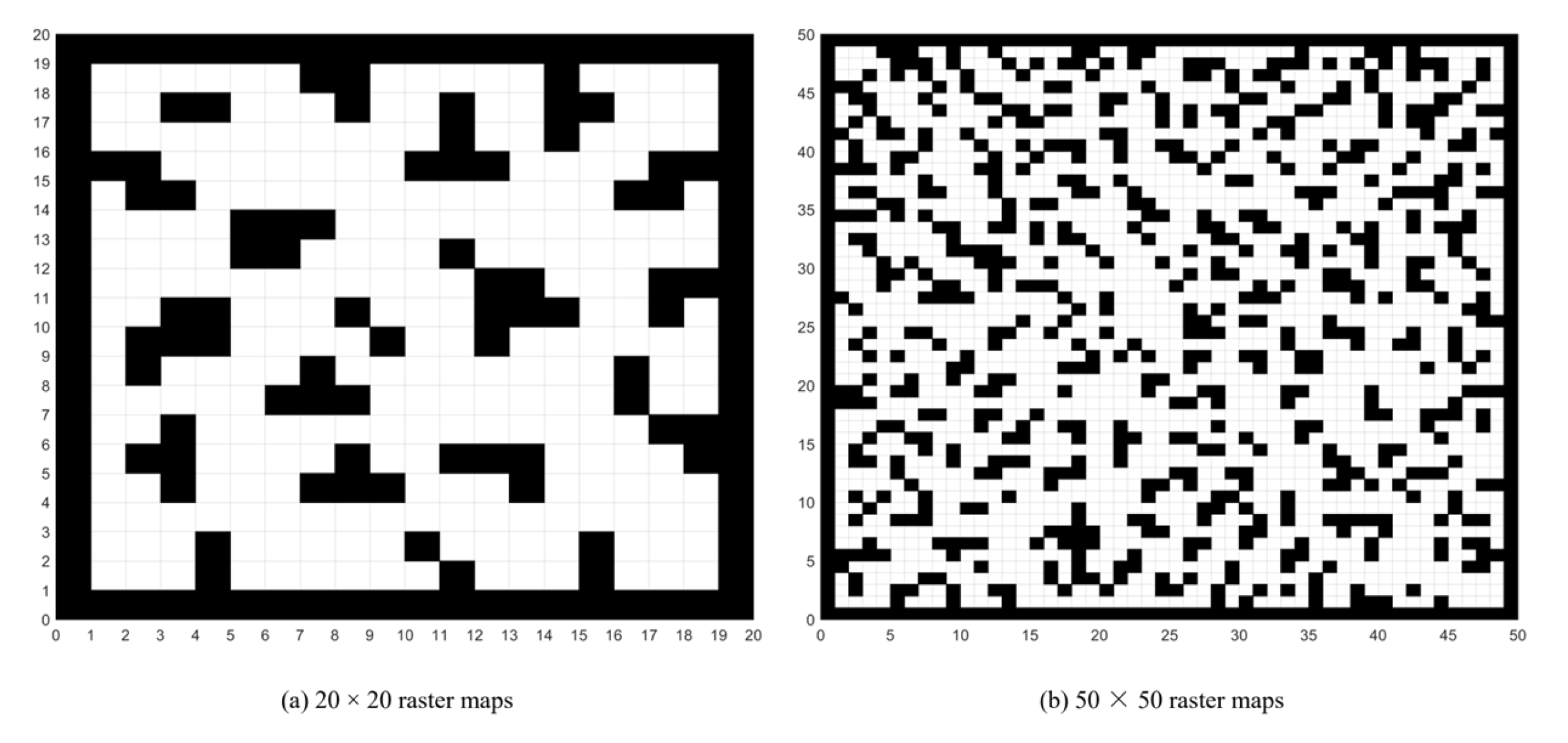
2.1. Establishment of Environmental Modeling
2.2. Traditional A* Algorithm
- (1)
- When the difference between the estimated generation value of the heuristic function and the actual value is large, the search space becomes larger.
- (2)
- The size of AGV is not considered but is simplified to a point, which may lead to the collision of AGV with obstacles.
- (3)
- There are too many inflection points in the path, which increases the difficulty of AGV operation.
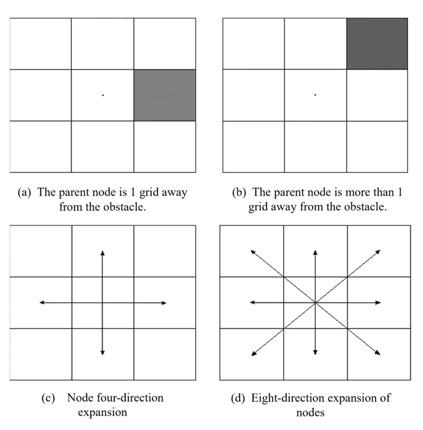
2.3. Improved A* Algorithm
2.3.1. Optimization of the Evaluation Function
2.3.2. Optimization of the Evaluation Function
2.3.3. Optimization of Key Points Extraction
3. DWA Algorithm and Improvements
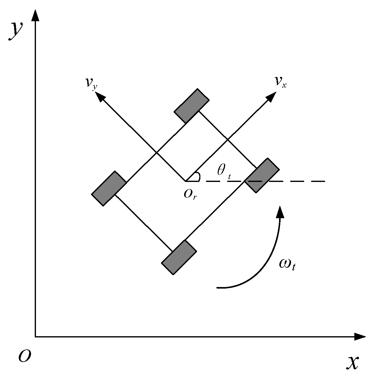
3.1. AGV Motion Model
3.2. Speed Sampling
- (1)
- The speed constraint of the AGV is expressed as in Equation (5).
- (2)
- In the predicted time range, the speed set under the constraint of acceleration and deceleration of the motor is expressed as in Equation (6).
- (3)
- When the AGV encounters a moving obstacle, it is necessary to ensure a safe distance between the AGV and the obstacle so that the speed of the AGV is reduced to zero before hitting the obstacle and its speed constraint is expressed as in Equation (7).
3.3. Optimization of the Evaluation Function
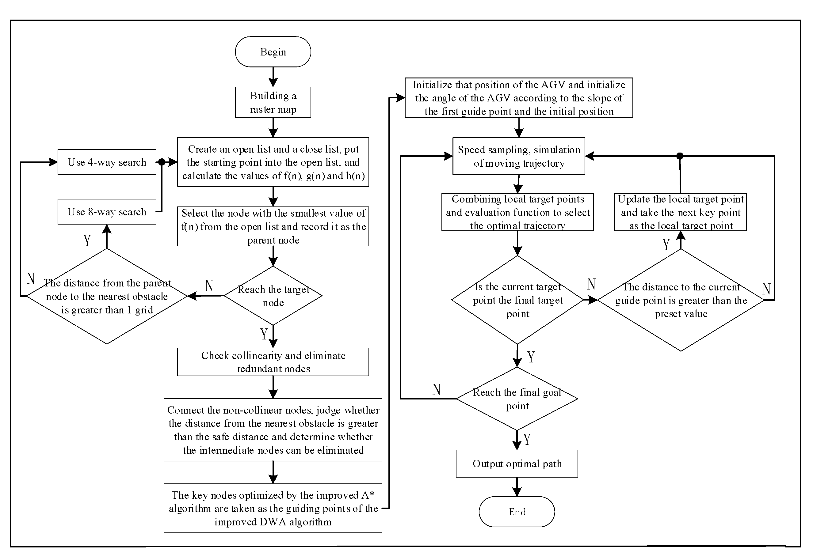
4. Fusion Algorithms
5. Simulation Analysis
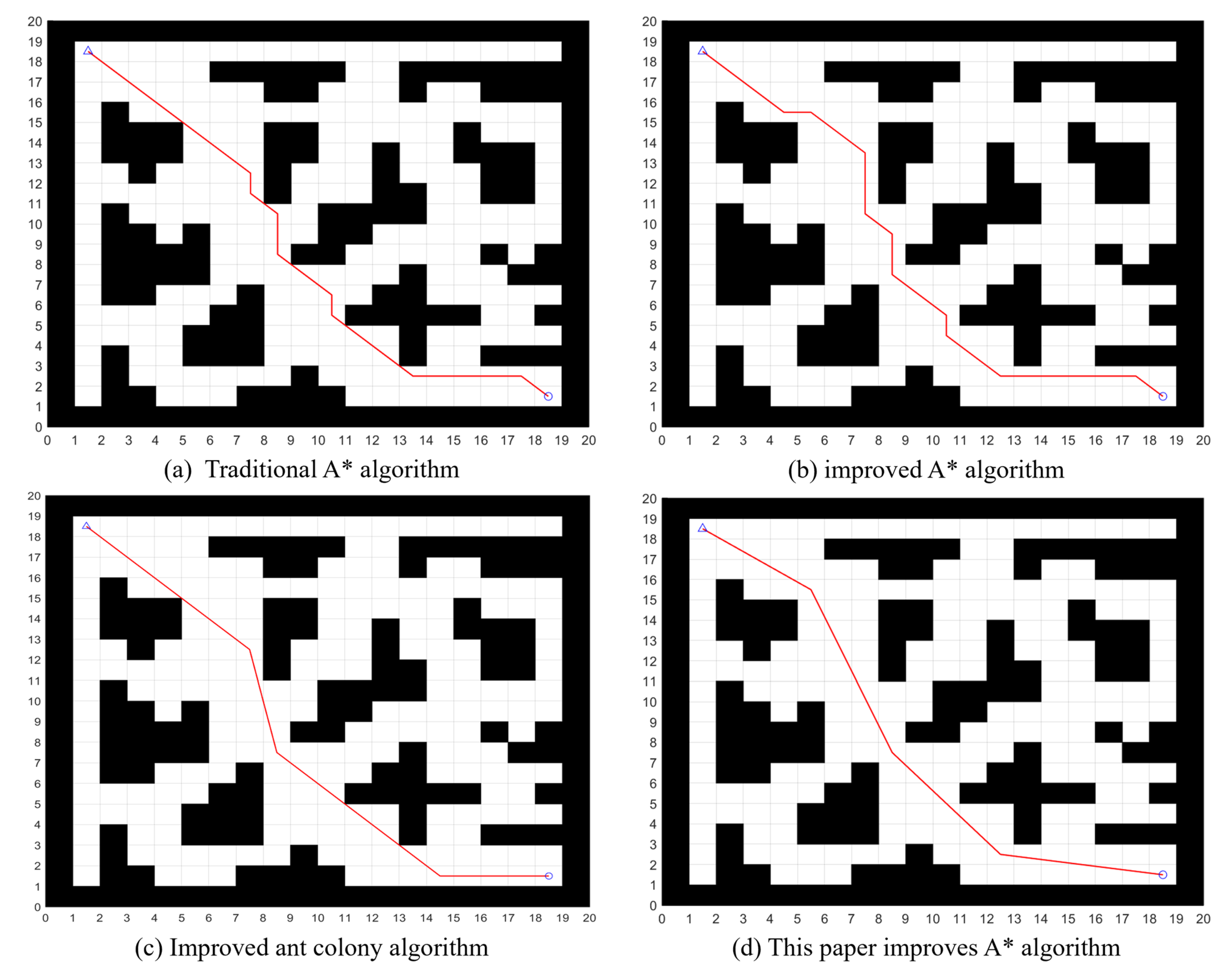
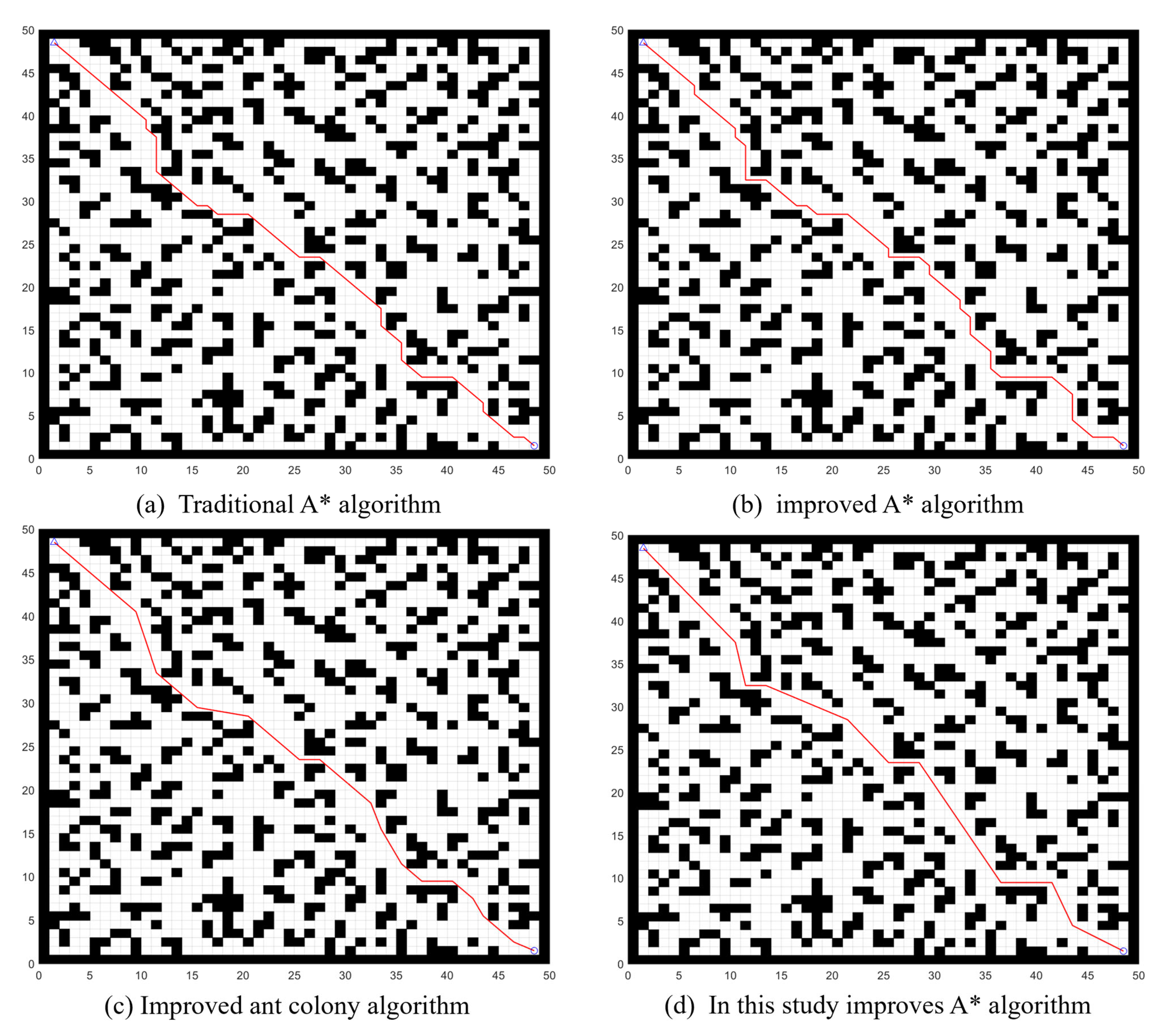
5.1. Simulation Results and Analysis of Improved A* Algorithm
5.2. Simulation Results and Analysis of Fusion Algorithm
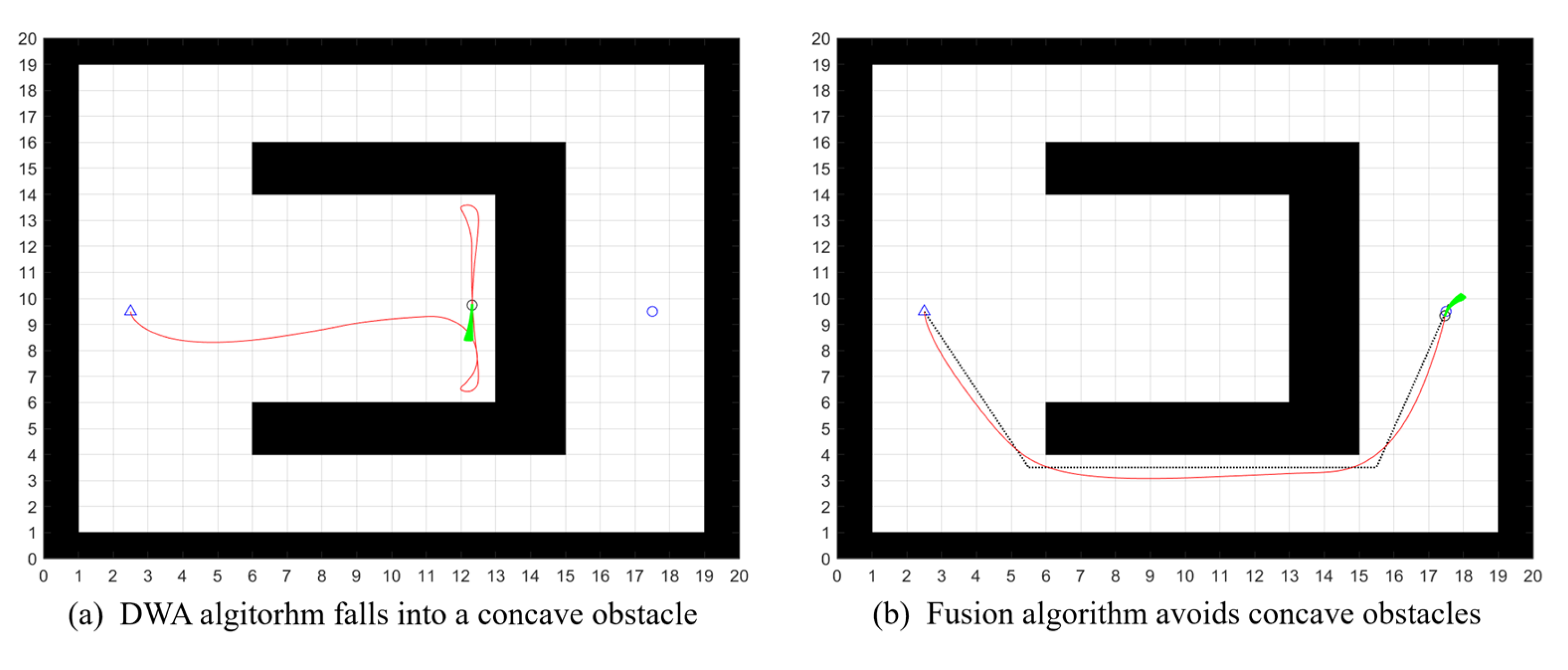
5.2.1. The Necessity of Algorithm Fusion
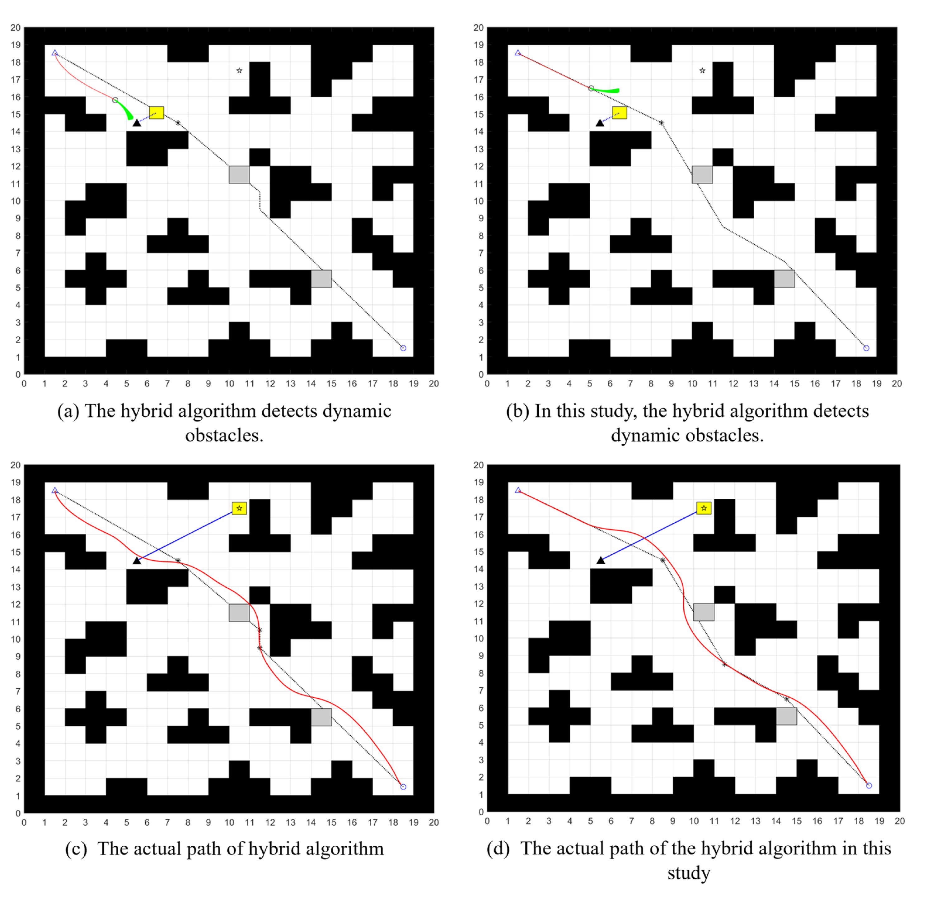
5.2.2. Simulation under Temporary Static Obstacle Environments
5.2.3. Simulation under Dynamic and Temporary Static Obstacle Environments
6. Conclusions
Author Contributions
Funding
Institutional Review Board Statement
Informed Consent Statement
Data Availability Statement
Conflicts of Interest
References
- Scellato, S.; Fortuna, L.; Frasca, M.; Gómez-Gardeñes, J.; Latora, V. Traffic optimization in transport networks based on local routing. Eur. Phys. J. B 2010, 73, 303–308. [Google Scholar] [CrossRef]
- Song, X.; Gao, H.; Ding, T.; Gu, Y.; Liu, J.; Tian, K. A Review of the Motion Planning and Control Methods for Automated Vehicles. Sensors 2023, 23, 6140. [Google Scholar] [CrossRef]
- Wang, H.; Hao, C.; Zhang, P.; Yin, P.; Zhang, Y. Path Planning of Mobile Robots Based on A* Algorithm and Artificial Potential Field Algorithm. China Mech. Eng. 2019, 30, 2489–2496. [Google Scholar]
- Duan, H.; Wu, Y.; Liu, J. Path planning of reconfigurable robot based on improved A* algorithm. Electron. Meas. Technol. 2023, 46, 44–50. [Google Scholar]
- Guo, Q.; Zhang, Z.; Xu, Y. Path-Planning of Automated Guided Vehicle Based on Improved Dijkstra Algorithm. In Proceedings of the 2017 Chinese Control and Decision Conference, Chongqing, China, 28–30 May 2017. [Google Scholar]
- Gbadamosi, O.A.; Aremu, D.R. Design of a Modified Dijkstra’s Algorithm for finding alternate routes for shortest-path problems with huge costs. In Proceedings of the 2020 International Conference in Mathematics, Computer Engineering and Computer Science (ICMCECS), Lagos, Nigeria, 18–21 March 2020. [Google Scholar]
- Xiao, J.; Yu, X.; Zhou, G.; Sun, K.; Zhou, Z. An improved ant colony algorithm for indoor AGV path planning. Chin. J. Sci. Instrum. 2022, 43, 277–285. [Google Scholar]
- Jiang, M.; Wang, F.; Ge, Y.; Sun, L. Research on path planning of mobile robot based on improved ant colony algorithm. Chin. J. Sci. Instrum. 2019, 40, 113–121. [Google Scholar]
- Wu, X.; Bai, J.; Hao, F.; Cheng, G.; Tang, Y.; Li, X. Field Complete Coverage Path Planning Based on Improved Genetic Algorithm for Transplanting Robot. Machines 2023, 11, 659. [Google Scholar] [CrossRef]
- Zheng, L.; Yu, W.; Li, G.; Qin, G.; Luo, Y. Particle Swarm Algorithm Path-Planning Method for Mobile Robots Based on Artificial Potential Fields. Sensors 2023, 23, 6082. [Google Scholar] [CrossRef] [PubMed]
- Jia, H.; Wei, Z.; He, X.; Zhang, L.; He, J.; Mu, Z. Path Planning Based on Improved Particle Swarm Optimization Algorithm. Trans. Chin. Soc. Agric. Mach. 2018, 49, 371–377. [Google Scholar]
- Lu, C.; Liang, S.; Jiang, C.; Dai, Y. Reinforcement based mobile robot path planning with improved dynamic window approach in unknown environment. Auton. Robot. 2020, 45, 51–76. [Google Scholar]
- Zhang, Y.; Song, J.; Zhang, Q. Local Path Planning of Outdoor Cleaning Robot Based on an Improved DWA. Robot 2020, 42, 617–625. [Google Scholar]
- Hu, Z.; Xu, B. Dynamic Path Planning Based on the Integration of A* Algorithm and Artificial Potential Field Method. Modul. Mach. Tool Autom. Manuf. Tech. 2023, 46–49+56. [Google Scholar] [CrossRef]
- Wang, B.; Wu, H.; Niu, X. Robot Path Planning Based on Improved Potential Field Method. Comput. Sci. 2022, 49, 196–203. [Google Scholar]
- Wen, Y.; Huang, J.; Jiang, T.; Su, X. Safe and smooth improved time elastic band trajectory planning algorithm. Control Decis. 2022, 37, 2008–2016. [Google Scholar]
- Jiang, Y.; Zhang, Y. Improved path planning of A* algorithm of domain node search strategy 8. J. Electron. Meas. Instrum. 2022, 36, 234–241. [Google Scholar]
- Zhao, X.; Wang, Z.; Huang, C.; Zhao, Y. Mobile Robot Path Planning Based on an Improved A*Algorithm. Robot 2018, 40, 903–910. [Google Scholar]
- Zhang, X.; Zou, Y. Collision-free path planning for automated guided vehicles based on improved A* algorithm. Syst. Eng.-Theory Pract. 2021, 41, 240–246. [Google Scholar]
- Zhang, H.; Zhang, Y.; Liang, R.; Yang, T. Energy efficient path planning method for robots based on improved A* algorithm. Syst. Eng. Electron. 2023, 45, 513–520. [Google Scholar]
- Chen, R.; Wen, C.; Peng, L.; You, C. Application of improved A* algorithm in indoor path planning for mobile robot. J. Comput. Appl. 2019, 39, 1006–1011. [Google Scholar]
- Mai, X.; Li, D.; Ouyang, J.; Luo, Y. An improved dynamic window approach for local trajectory planning in the environment with dense objects. J. Phys. Conf. Ser. 2021, 1884, 360–369. [Google Scholar] [CrossRef]
- Wang, Y.; Tian, Y.; Li, X.; Li, L. Self-adaptive dynamic window approach in dense obstacles. Control. Decis. 2019, 34, 927–936. [Google Scholar]
- Chang, L.; Shan, L.; Dai, Y.; Qi, Z. Multi-robot formation control in unknown environment based on improved DWA. Control. Decis. 2022, 37, 2524–2534. [Google Scholar]
- Li, X.; Liu, F.; Liu, J.; Liu, J.; Liang, S. Obstacle avoidance for mobile robot based on improved dynamic window approach. Turk. J. Electr. Eng. Comput. Sci. 2017, 25, 666–676. [Google Scholar] [CrossRef]
- Wang, Z.; Chen, X. Path Planning Algorithm Based on Improved A* and DWA for Unmanned Surface Vehicle. Chin. J. Sens. Actuators 2021, 34, 249–254. [Google Scholar]
- Li, X.; Fang, J. Research on UAV path planning by A* algorithm and DWA method in the urban environment. Unmanned Syst. Technol. 2023, 6, 61–70. [Google Scholar]
- Lao, C.; Li, P.; Feng, Y. Path Planning of Greenhouse robot Based on Fusion of Improved A* Algorithm and Dynamic Window Approach. Trans. Chin. Soc. Agric. Mach. 2021, 52, 14–22. [Google Scholar]
- Zhao, J.; Zhao, T.; Feng, Y.; Cao, Z.; Zhong, Y. Research on robot path planning based on improved A* algorithm and DWA. Exp. Technol. Manag. 2023, 40, 87–92. [Google Scholar]
- Chi, X.; Li, H.; Fei, J. Research on robot random obstacle avoidance method based on fusion of improved A*algorithm and dynamic window method. Chin. J. Sci. Instrum. 2021, 42, 132–140. [Google Scholar]
- Zhang, Z.; Zhang, H.; Deng, Y. Real Time Path Planning of Robot by Combing Improved A∗ Algorithm and Dynamic Window Approach. Radio Eng. 2022, 52, 1984–1993. [Google Scholar]
- Zou, W.; Han, B.; Li, P.; Tian, J. Path planning based on the integration of improved A* algorithm and optimized dynamic window approach. In Computer Integrated Manufacturing Systems; Prentice-Hall, Inc.: Hoboken, NJ, USA, 1995; pp. 1–18. [Google Scholar]
- Wei, G.; Zhang, J. Research on Unmanned Surface Vessel Aggregation Formation Based on Improved A* and Dynamic Window Approach Fusion Algorithm. Appl. Sci. 2023, 13, 8625. [Google Scholar] [CrossRef]
- Chen, J.; Xu, L.; Chen, J.; Liu, Q. Path planning based on improved A* and dynamic window approach for mobile robot. Comput. Integr. Manuf. Syst. 2022, 28, 1650–1658. [Google Scholar]
- Wu, M.; Gao, J.; Li, L.; Wang, Y. Control optimisation of automated guided vehicles in container terminal based on Petri network and dynamic path planning. Comput. Electr. Eng. 2022, 104, 108471. [Google Scholar] [CrossRef]


| AGV Motion Parameters | |||
|---|---|---|---|
| Maximum linear velocity | 2 m/s | Maximum linear acceleration | 0.2 m/s2 |
| Maximum angular velocity | 20°/s | Maximum angular acceleration | 50°/s2 |
| Velocity resolution | 0.01 m/s | Speed resolution | 1°/s |
| Algorithm | Path Length (m) | Turning Times | Total Turning Angle |
|---|---|---|---|
| Traditional A* | 26.38 | 8 | 360.0 |
| [21] | 27.56 | 20 | 450.0 |
| [8] | 26.07 | 3 | 112.4 |
| This study improves A* | 26.03 | 3 | 79.8 |
| Algorithm | Path Length (m) | Turning Times | Total Turning Angle |
|---|---|---|---|
| Traditional A* | 72.33 | 20 | 900.0 |
| [21] | 75.84 | 28 | 1260.0 |
| [8] | 70.49 | 14 | 410.0 |
| This study improves A* | 72.00 | 9 | 435.3 |
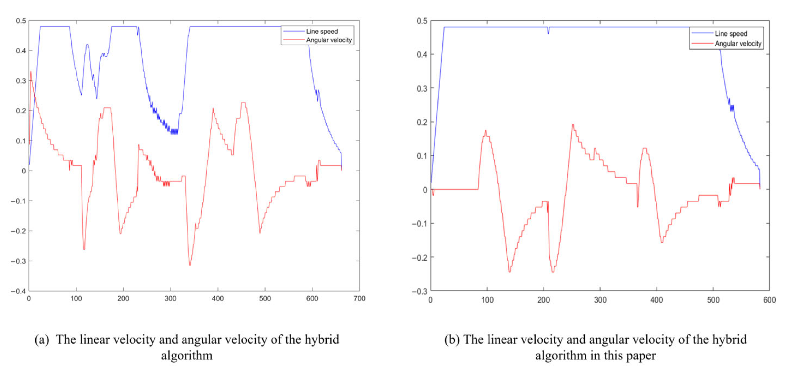
| Algorithm | Path Length (m) | Run Time (s) |
|---|---|---|
| [22] | 25.49 | 123.97 |
| Hybrid algorithm in this study | 25.47 | 108.34 |
Disclaimer/Publisher’s Note: The statements, opinions and data contained in all publications are solely those of the individual author(s) and contributor(s) and not of MDPI and/or the editor(s). MDPI and/or the editor(s) disclaim responsibility for any injury to people or property resulting from any ideas, methods, instructions or products referred to in the content. |
© 2023 by the authors. Licensee MDPI, Basel, Switzerland. This article is an open access article distributed under the terms and conditions of the Creative Commons Attribution (CC BY) license (https://creativecommons.org/licenses/by/4.0/).
Share and Cite
Guo, T.; Sun, Y.; Liu, Y.; Liu, L.; Lu, J. An Automated Guided Vehicle Path Planning Algorithm Based on Improved A* and Dynamic Window Approach Fusion. Appl. Sci. 2023, 13, 10326. https://doi.org/10.3390/app131810326
Guo T, Sun Y, Liu Y, Liu L, Lu J. An Automated Guided Vehicle Path Planning Algorithm Based on Improved A* and Dynamic Window Approach Fusion. Applied Sciences. 2023; 13(18):10326. https://doi.org/10.3390/app131810326
Chicago/Turabian StyleGuo, Tao, Yunquan Sun, Yong Liu, Li Liu, and Jing Lu. 2023. "An Automated Guided Vehicle Path Planning Algorithm Based on Improved A* and Dynamic Window Approach Fusion" Applied Sciences 13, no. 18: 10326. https://doi.org/10.3390/app131810326