Article

Platooning Cooperative Adaptive Cruise Control for Dynamic Performance and Energy Saving: A Comparative Study of Linear Quadratic and Reinforcement Learning-Based Controllers

1
Department of Energy (DENERG), Politecnico di Torino, 10129 Torino, Italy
2
Department of Mechanical and Aerospace Engineering (DIMEAS), Politecnico di Torino, 10129 Torino, Italy
*
Author to whom correspondence should be addressed.
Appl. Sci. 2023, 13(18), 10459; https://doi.org/10.3390/app131810459
Submission received: 7 July 2023 / Revised: 6 September 2023 / Accepted: 12 September 2023 / Published: 19 September 2023

Abstract

:
In recent decades, the automotive industry has moved towards the development of advanced driver assistance systems to enhance the comfort, safety, and energy saving of road vehicles. The increasing connection and communication between vehicles (V2V) and infrastructure (V2I) enables further opportunities for their optimisation and allows for additional features. Among others, vehicle platooning is the coordinated control of a set of vehicles moving at a short distance, one behind the other, to minimise aerodynamic losses, and it represents a viable solution to reduce the energy consumption of freight transport. To achieve this aim, a new generation of adaptive cruise control is required, namely, cooperative adaptive cruise control (CACC). The present work aims to compare two CACC controllers applied to a platoon of heavy-duty electric trucks sharing the same linear spacing policy. A control technique based on reinforcement learning (RL) algorithm, with a deep deterministic policy gradient, and a classic linear quadratic control (LQC) are investigated. The comparative analysis of the two controllers evaluates the ability to track inter-vehicle distance and vehicle speed references during a standard driving cycle, the string stability, and the transient response when an unexpected obstacle occurs. Several performance indices (i.e., acceleration and jerk, battery state of charge, and energy consumption) are introduced as metrics to highlight the differences. By appropriately selecting the reward function of the RL algorithm, the analysed controllers achieve similar goals in terms of platoon dynamics, energy consumption, and string stability.

1. Introduction

The growing need to improve road safety has led the automotive industry to develop advanced driver assistance systems (ADAS), which significantly contribute to the reduction and mitigation of accidents [1]. On the other hand, the efficient use of energy for vehicle propulsion has become the main driver for the research and development of novel powertrains; it is worth mentioning that the automotive sector greatly contributes to the global production of polluting emissions [2]. In the context of automated driving, vehicle platooning represents an enabling technology for both increased occupant safety and energy savings. Vehicle platooning has been extensively studied in the last decades as it represents a suitable method for reducing the energy consumption and greenhouse gas emissions of heavy-duty vehicles. Different platooning test projects (e.g., Chauffeur, Sartre, Energy-ITS, SCANIA) were carried out in different countries to investigate different platooning systems [3,4], vehicle mixes, types of infrastructure, and sensors. The focus of these projects was to investigate the potential for energy consumption reduction and an increase in road capacity, the latter representing a key task of the transportation sector.
The advantages linked to drag reduction represent a key aspect in the scientific community [5,6,7]. The research efforts highlighted that heavy-duty vehicles (HDV) are the most indicated for energy-oriented platooning, given that they can exploit the benefits of the slipstream effect for viable inter-vehicle distances. On the contrary, this effect cannot be exploited by light-duty vehicles unless the inter-vehicle distance is less than 3 m. Still, driving close to the previous vehicle leads to safety concerns; thus, trade-off conditions or dedicated systems need to be carefully investigated. More specifically, in [8], multi-vehicle collision avoidance strategies using active emergency braking systems were developed to improve the safety of a string of vehicles in complex scenarios by also gathering information from the infrastructure. The safety issue can also be managed through the selection of a proper spacing policy that links the vehicle speed to the inter-vehicular distance. The author of [9] performed a comparative study of five different spacing policies by analysing the performances in terms of stability, comfort, and safety for adaptive cruise control systems.
To accomplish the cooperative task of platooning control, cooperative adaptive cruise control (CACC) has been developed; unlike classic ACC, it gathers information from all vehicles in the string, i.e., distance, velocity, and accelerations. The exchange of data relies on vehicle-to-everything (V2X) and/or vehicle-to-vehicle (V2V) technology. The main disadvantage of the classic ACC is that string stability is not ensured, as demonstrated by the on-field test in [10], where the adaptive cruise control of several vehicles was tested. On the contrary, CACC systems guarantee string stability, as demonstrated by the authors of [11], where the focus was to design and validate a CACC system. Moreover, string stability can also be guaranteed by a proper design of the spacing policy. In [12], string stability was investigated by developing a delay-based spacing policy that guarantees the same speed profile in a spatial domain.
In the literature, the cooperative strategy has been implemented using different algorithms. The authors of [13] developed a proportional string stable feedback control strategy by using information on distance and speed errors; the study proved to be feasible through an experimental validation conducted over a platoon of trucks. Other works have used more advanced control techniques, as done by the authors of [14], where a model predictive control (MPC) strategy, combined with the topography information responsible for generating efficient speed profiles, was deployed to drive vehicle platoons. Moreover, in [15], the comparison between nonlinear MPC and proportional-integrative-derivative (PID) controllers was investigated to optimise fuel consumption and guarantee the safety of a class of eight trucks over hilly terrain.
Among these different approaches, in this paper, a centralised control system is developed to drive a platoon of vehicles along a straight path, designed to target energy saving, safety, and dynamic performance by investigating two control techniques: a classic one used as a reference, represented by the linear quadratic controller (LQC), and a novel one based on the reinforcement learning (RL) algorithm. The LQC strategy has been selected due to its capability to guarantee system stability as well as its fast tuning process and fast computational time. On the other hand, RL was selected as an emerging technology with high innovative potential. RL is a promising control technique for CACC algorithms because it guarantees adaptability to different situations and the possibility to continue its training online; moreover, it has proven to be particularly effective in handling uncertain and hard-to-predict environments. Generically speaking, RL allows us to directly handle the nonlinear dynamics of physical systems. If the training phase is properly designed, an RL-based CACC system can learn how to adapt to the inherent variability in aspects such as road conditions, traffic patterns, and driver behaviour.
Furthermore, the potential of RL solutions has been widely assessed in the scientific literature. The control of a vehicle platoon has a large action and state space, thus making deep RL (DRL)-based solutions suitable for the problem [16,17,18,19]. Moreover, the chosen DRL approach is model-free, i.e., it does not require a model to predict the behaviour of the system as opposed to model-predictive control (MPC) [20]. It is also worth observing that whereas LQC requires a quadratic objective function, DRL does not hold any constraint on the reward function shape, which can also be a non-quadratic cost function. Yet, differently from other analytical control methods, DRL-based control cannot theoretically guarantee convergence or system stability. It is indeed a non-linear control that learns through interaction with an environment, pairing the action evaluated to be the best for a given state with the state itself through the experience gained during training. Thus, its performance cannot be mathematically or theoretically guaranteed since it depends not only on the mathematical formulation but also on the training duration and other parameter settings. Further information can be found in Section 4, where the DRL-based control is described.
The paper is divided as follows: in Section 2, the vehicle platoon model is presented; in Section 3 and Section 4, the LQC and RL architectures are respectively introduced. In Section 5, the results of platoon simulation, tracking an FTP75 driving cycle, and a cut-in scenario are presented with the aim of comparing the CACC controllers by means of a set of performance, energy, and safety indices. Finally, the conclusions of the research are reported in Section 6.

2. Model Description

2.1. Vehicle Model

In this section, the platoon model is introduced. A number of N heavy-duty electric vehicles (HDEVs) moving on a straight and sloped road is considered. Figure 1 shows the scheme of the mechanical model of the vehicle platoon: the dark blue vehicle is called the lead vehicle, whereas the others are referred to as the followers.
Each vehicle is characterised by inertial and geometrical properties: a mass m i and the total vehicle length l i . Only the longitudinal motion is accounted for, whereas the lateral and pitch ones are neglected. The position, velocity, and acceleration ( x i , v i , v ˙ i ) of each vehicle are computed by using a fixed reference system X . The quantity d i 1 , i refers to the inter-vehicle distance (i.e., the distance between the rear and front bumpers of two consecutive vehicles). The electric motor provides the amount of torque necessary to overcome the rolling, aerodynamic, and climbing resistances, as well as the inertial torque for vehicle and powertrain acceleration. The amount of torque is computed by the control system, and it is transmitted to the driveshafts by a single-speed transmission, modelled as a constant transmission ratio and assuming rigid shafts.
Even though the pure rolling motion is assumed for each wheel, the actual tyre-road friction condition has been considered by implementing a simple traction control system that saturates the tyre forces to their maximum transmissible limit, depending on road grip μ and the normal load F z . In this way, the tyres never exceed their maximum transmissible force, F x < μ F z .
The equation of motion of the i t h vehicle is:
m t o t i v ˙ F , i = η τ T m , i r w , i m i g s i n α + m i g f 0 , i c o s ( α ) + m i g f 2 , i cos α + 1 2 ρ c x , i ( d i 1 , i ) A f , i v F , i 2
where m t o t , i is the equivalent translating mass of the vehicle, accounting for the translating and rotating components, f 0 , i and f 2 , i are the rolling resistance coefficients that are generally characterised experimentally through quadratic regression applied to the coast-down test, r w , is the wheel rolling radius, τ and η are the reduction ratio and the efficiency of the transmission, ρ is the air density, A f , i is the vehicle frontal area, c x , i is the aerodynamic drag coefficient, and α represents the longitudinal road slope.
Once the torque requested for the electric motor is known, the power request can be derived as the aforementioned torque multiplied by the angular velocity of the motor. Electric motor losses are modelled as a function of their torque and speed through a 2D map. The power absorbed by the auxiliaries is assumed to be constant. The battery power request is the sum of the electric motor power and the abovementioned contributions. The behaviour of the battery is represented by the following equations, which evaluate the amount of current flowing through the battery and the instantaneous change in the state of charge ( σ ˙ ):
I b a t t = V b a t t V b a t t 2 4 R b a t t P b a t t 2 R b a t t
σ ˙ = I b a t t Q b a t t · t
where I b a t t is the battery current, V b a t t and R b a t t are its open-circuit voltage and internal resistance, and Q b a t t and Δ t are the battery maximum capacity and the simulation timestep, respectively.
The dependency of the drag reduction on the inter-vehicle distance, which was experimentally validated for HDVs in [21], is introduced in the model with the following equations:
c x , i = c x , 0 k c x
k c x = 1 Δ C x Δ C x % = 1 a 3 , i d 3 + a 2 , i d 2 , a 1 , i d + a 0 , i b 3 , i d 3 + b 2 , i d 2 + b 1 , i d + b 0 , i × 100
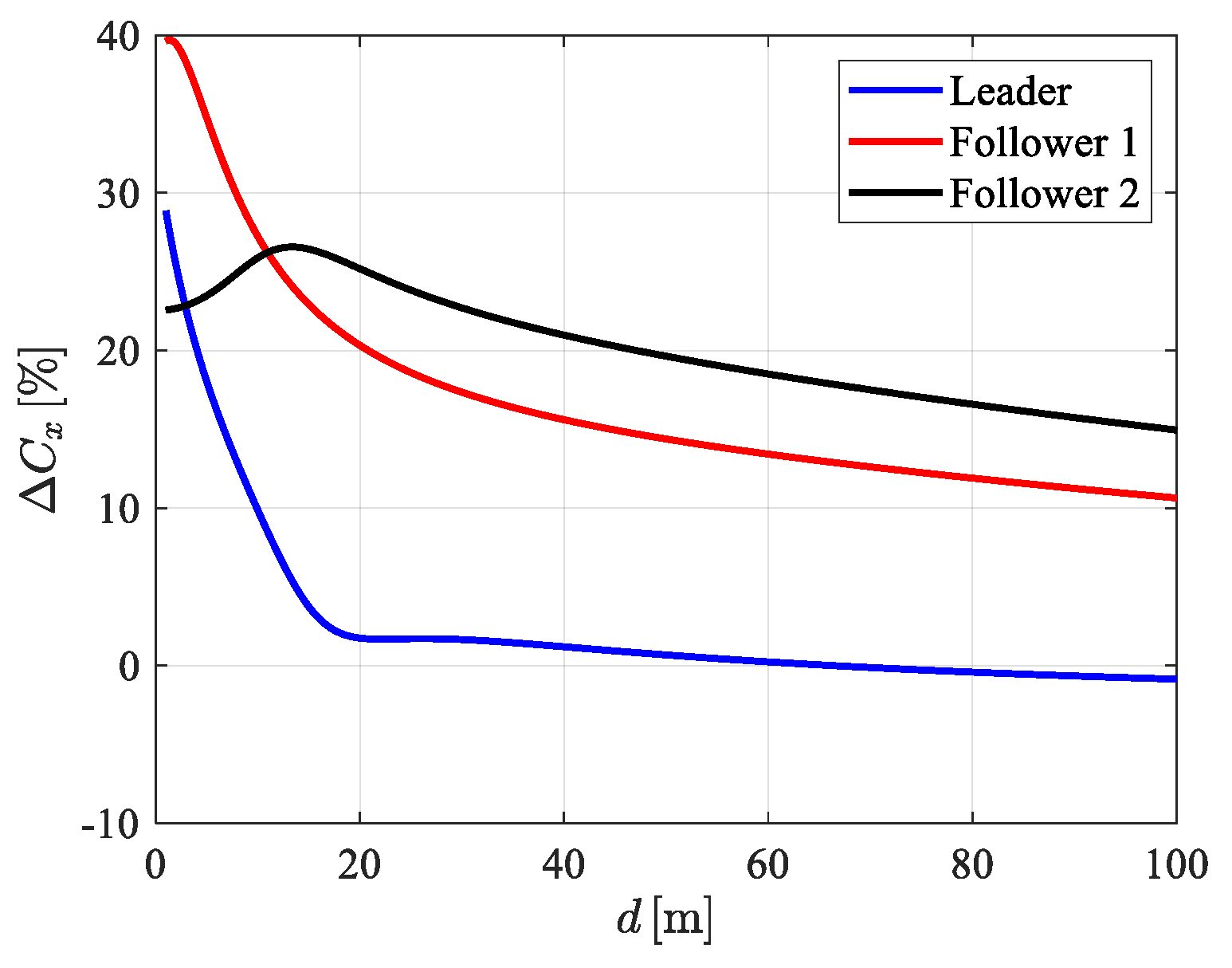
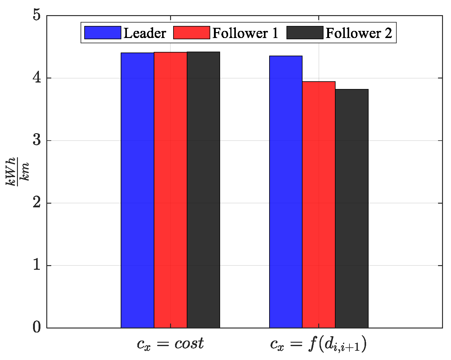
where d represents the relative distance, c x , 0 is the undisturbed drag coefficient (i.e., the drag coefficient of the isolated vehicle), and a n , i and b n , i are empirical coefficients obtained by experimental data fitting [21]. Figure 2 shows the trend of the drag coefficient reduction versus the inter-vehicle distance for a platoon composed of three HDVs. It is noticeable that the middle (red line) and last (black line) vehicles are more affected by the drag reduction than the leader. The map, derived from the literature, was included in the platoon model to evaluate the potential for energy savings. Figure 3 shows the energy consumption comparison related to a set of three trucks following a WLTP Class 3 driving cycle: the group of bars on the left represents the vehicles moving far enough apart not to be affected by the slipstream of the preceding vehicle, while the bars on the right refer to the same vehicles moving close together thanks to a platoon control system. The results demonstrate that each vehicle in the platoon shows energy savings; in particular, the advantage increases from the first to the last vehicle. Obviously, the quantitative results depend on vehicle data and platooning control parameters; Figure 3 refers to the numerical values used in Section 5.
The inter-vehicle distance and its derivative are defined as:
d i 1 , i = x i 1 x i l i 1 d ˙ i 1 , i = v i 1 v i
The vehicle platooning control system is conceived to exploit the advantages of a collaborative ACC. More specifically, the test scenario is based on a lead vehicle following the reference speed of a driving cycle, thanks to a PID controller, whereas the string of followers is controlled by a centralized control unit, which exploits the information from the sensors, i.e., vehicle velocity v i and inter-vehicle distance d i 1 , i , to track a reference value of inter-vehicle distance (according to the spacing policy) and a target speed of the platoon. The reference values are computed by the centralised controller, which in turn evaluates the amount of torque to be applied by each actuator in the platoon in order to compensate for the velocity and distance errors. All the data exchange (feedback signals, references, and inputs) is instantaneous. Thus, neither delay nor disturbance are accounted for.
The idea of a centralised control unit is investigated considering two different control solutions: the linear quadratic controller (LQC) and a reinforcement learning-based controller (RL).

2.2. Spacing Policy

To maintain a safe distance between vehicles, a spacing policy must be properly defined. Different solutions may be adopted, from the simplest one (e.g., maintaining the safety distance constant) to more complex ones (e.g., including the velocity or acceleration terms in the safety distance) [9]. In this paper, the safety distance, also referred to as the inter-vehicle safety distance, is set by the following law:
d i 1 , i , r e f = d 0 + t h v i
where d 0 represents the minimum distance between vehicles (when the vehicles are stationary), t h is the time headway, and v i is the speed of the i t h vehicle. Consistent with Equation (7), a constant time headway implies a safety distance growing linearly with velocity. Reference [22] suggests time headway in the interval [1 s, 2 s], based on safety and road capacity concerns.

3. LQ Controller

3.1. Open Loop System: Model Linearization

The linear quadratic controller (see [23,24] for more details on this well-established technique) was chosen since it fits very well with the multi-input, multi-output requirement of the centralised collaborative platooning controller. To apply this technique, the platoon model was linearized and the resulting equations of motion stacked in state–space form. Before linearization, the equations are normalised to the nominal condition by introducing:
d i 1 , i = d n z F i , d v F , i = v n z F i , v α = α n p T m , F , i = T m , n u
where v n , d n , T m , n are the nominal velocity, the nominal inter-vehicle distance, and the nominal electric motor torque, respectively; z i , d and z i , v are the states of each follower vehicle; u represents the input; and p represents the road slope disturbance.
Introducing the normalisation from (1), the equation of motion can be written:
m t o t i v n z ˙ F i , 2 = T m , n τ η r w u A 0 sin α n p + A 1 cos α n p + B 0 cos α n p + B 1 + B 2 d n z F i , d v n 2 z F i , v 2
where the expressions of the A 0 , A 1 , B 0 , B 1 , B 2 are shown in Appendix A.
At steady state ( z ˙ F i , v = 0 ) and without external disturbance ( p = 0 ) , the nominal torque is:
T m , n = r w η τ A 1 + B 0 + B 1 d n v n 2
Let us introduce the small variations, denoted with δ , around the nominal values:
z F i , d = 1 + δ z F i , d z F i , v = 1 + δ z F i , v u = 1 + δ u p = δ p
Thus, introducing the linearisation and neglecting the second-order variational terms, the linearised equation of motion for each follower vehicle is:
δ z F i , v = K i δ u i G i δ z F i , v S i δ z F i , d E i δ p
The time derivative of inter-vehicle (variational) distance can be written as:
δ z ˙ F i , d = v n d n δ z F i 1 , v δ z F i , v
Therefore, by applying the former steps for each follower vehicle, the final set of equations of motion of the vehicle platoon under open-loop control can be found:
{ δ z ˙ } = A δ z + B δ u + H δ p + C δ z L , v
where A ,   [ B ] are the dynamic and input matrices, respectively, { δ z } is the state vector:
δ z = δ z F 1 , d δ z F 1 , v δ z F i , d δ z F i , v δ z F N , d δ z F N , v
where δ z F i , d and δ z F i , v is the normalised variational distance and speed, { δ u } is the input vector, δ z L , v is the normalised variational lead vehicle velocity (internal disturbance), and { δ p } is the variational inclination contribution (external disturbance). The content of the matrices and the gains in a case study of three vehicles are given in Appendix A.

3.2. Control: Closed Loop System

The longitudinal dynamics of the follower vehicles are controlled in a closed loop using the LQC technique. The latter is based on the minimization of a quadratic functional and has the advantage of ensuring the asymptotic stability of the controlled system [23]. Since the LQC control law is a linear combination of all the states δ e , the equations are rearranged to have the errors of inter-vehicle distance δ e d i , i + 1 and vehicle velocity δ e v , i as states:
δ e = δ z δ z r e f
where δ z r e f is the reference vector of the desired speeds and desired inter-vehicle distances (normalised w.r.t. the nominal values and variational). Moreover, an augmented state η i , that is, the integral of the distance error ( η i ˙ = δ e d i , i + 1 ) , is added as the last element of the state vector to include an integral term in the full-state feedback control law, compensating for the steady state errors.
Therefore, the equations are entirely re-written by substituting the expression (19) in (15), leading to:
δ e ˙ = A δ e + B δ u + A δ z r e f δ z ˙ r e f + H δ p + C δ z 1 , v
The control law { δ u } is here defined as:
δ u = δ u F B + δ u F F
where δ u F B represents the feedback control term, whereas δ u F F represents the feedforward control term. The feedback control law is full-state feedback:
δ u F B = [ L ] { δ e }
where [ L ] is the control gain matrix, computed by solving the steady-state Riccati equation. This solution guarantees the minimization of the cost function J ( { δ u } ) , defined by the LQC problem:
J { δ u } = 0 δ e T Q δ e + δ u T R { δ u } d t
where Q and R are diagonal weight matrices that are tuned based on the desired system performance. More specifically, [ Q ] controls the deviation of the states from equilibrium, whereas R controls the input effort. In the next section, the tuning process for the matrices will be presented.
The feedforward contribution δ u F F is designed to compensate for the terms of Equation (16) that are not a linear combination of the states:
δ u F F = B + A δ z r e f + δ z ˙ r e f H δ p C δ z 1 , v
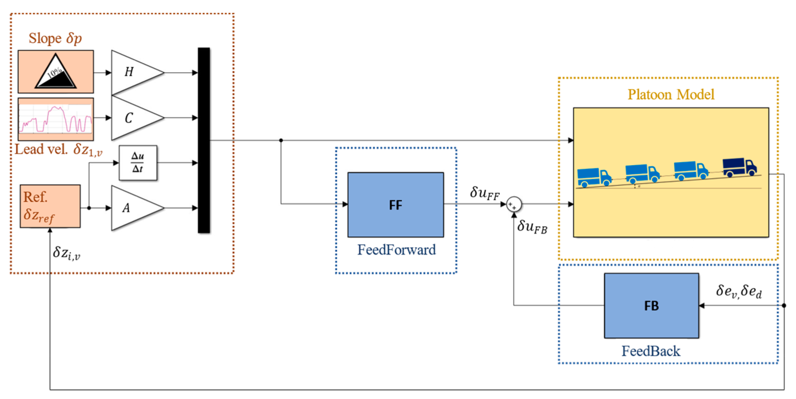
Since the input matrix [ B ] is not square and hence not invertible, B + indicates the pseudoinverse (or generalised inverse) matrix, computed with the Moore–Penrose method [25]. The existence and uniqueness of the pseudoinverse of the [ B ] matrix have been verified by checking the four Penrose conditions applied to the [ B ] matrix (see Appendix B for more details). Figure 4 shows the block diagram of the controlled platooning system. On the left are the input/disturbances applied to the dynamic system, i.e., the road slope, the velocity of the lead vehicle, and the reference speed and distance of each vehicle. The plant with the two controllers (feedback and feedforward) is shown in the central part and on the right of the figure.

3.2.1. Tuning of Q and R Matrices and Time Headway

The results achievable by the feedback control are affected by the choice of the weight matrices Q and R . In the adopted methodology, they were tuned to guarantee the best trade-off for the following objectives.
  • Comfortable drive: to ensure comfort for each vehicle, threshold values for longitudinal acceleration and jerk are set to a x < | 2 | m s 2 and d a x d t < | 0.9 | m s 3 , as specified by the authors of [26].
  • Safety: the control system must be able to safely stop each vehicle in the platoon, namely avoiding rear-end collisions, when an emergency braking condition occurs at the maximum speed permitted by the regulations, e.g., considering highway speed limits (80 km/h for HDVs).
A sensitivity analysis on the values of the matrix R was performed to facilitate the tuning process, aiming at satisfying the aforementioned objectives. The values of the Q matrix are kept fixed during sensitivity. The effect on safety and comfort of the time headway t h will also be presented. To maximize the overall efficiency of the platoon of vehicles, the time headway is set to maintain the vehicles at low inter-vehicle distances without compromising safety. The matrices were hence tuned by analysing two manoeuvres: WLTP Class 3 driving cycle and emergency braking. In the following sections, the results of a platoon composed of three trucks will be shown.

3.2.2. WLTP Class 3 Driving Cycle

The truck platoon is subjected to a WLTP Class 3 driving cycle. The nominal velocity v n is set to 80 km/h, and the nominal distance d n varies according to the time headway t h and d 0 settings: the latter is maintained constant at d 0 = 3   m . The lead vehicle’s speed is controlled using PID logic. The PID gains ( K P , K D , K I ) are set to K P = 300 , K D = 5 , K I = 10 . The remaining control parameters ( R 0 and t h ) are set according to Table 1, while the truck’s inertial and geometrical data are listed in Table 3. R 0 represents the constant weight of the [ R ] matrix ( [ R ] = R 0 [ I ] ), equal for both follower trucks.
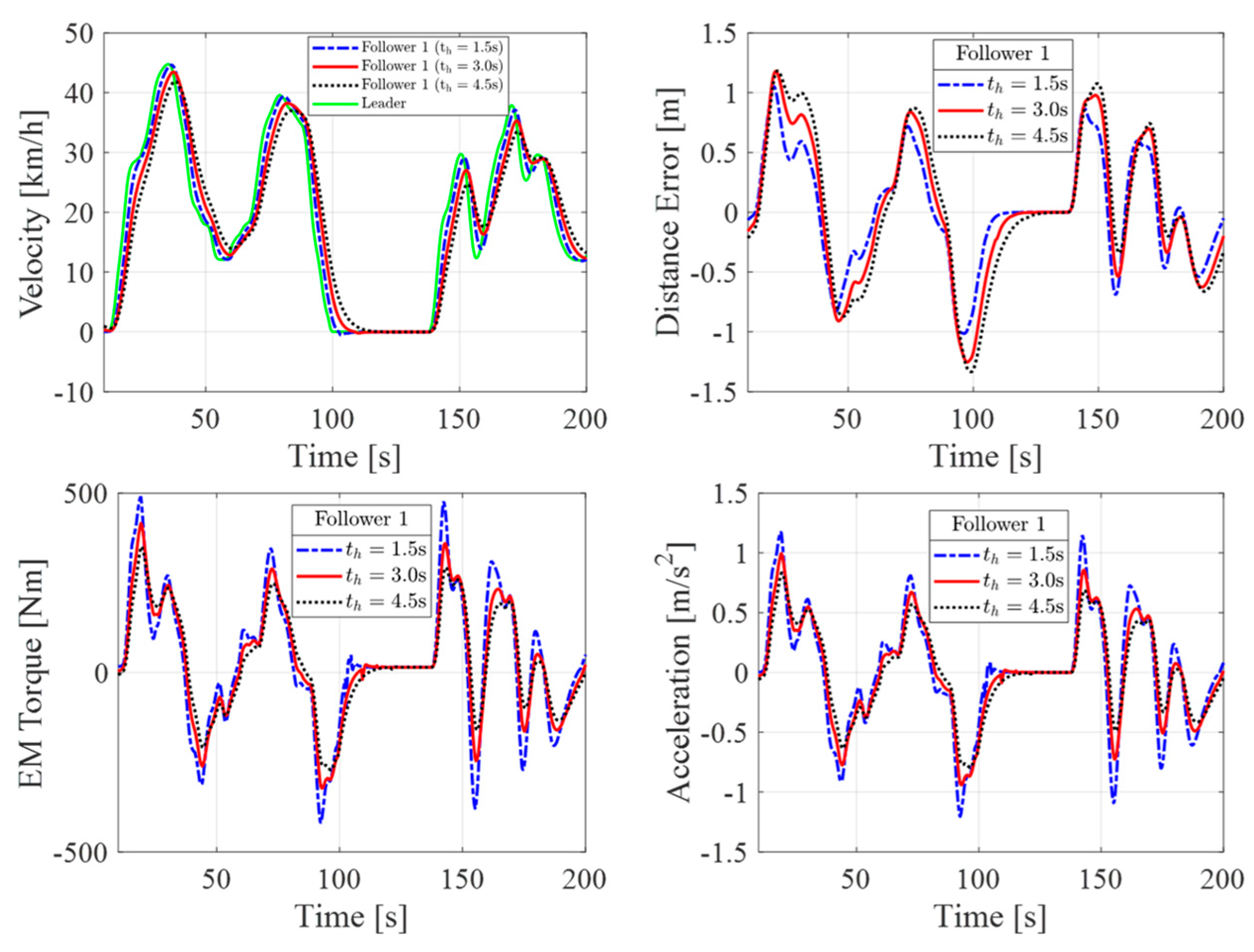
The results of the WLTP Class 3 driving cycle are divided into two parts: Figure 5 shows the R 0 sensitivity (with constant time headway t h = 1.5   s ), whereas Figure 6 depicts the t h sensitivity (with constant R 0 set to 10 5 ).
In Figure 5, the top charts report the velocity of follower 1 (left) and the inter-vehicle distance errors (namely e d 1,2 ), whereas the electric motor torque is reported in the bottom charts. The green line represents the vehicle leader velocity (the disturbance), whereas the follower 1 velocity response is represented for the three different analysed values of R 0 . The results show that, even though the difference in torques is quite small, the lower the R 0 values, the better the tracking inter-vehicle distance performance.
In Figure 6, the effect of the time headway is more evident in the results: the higher the time headway, the less motor torque is delivered, resulting in lower longitudinal acceleration. Therefore, higher values of time headway improve passenger comfort as the RMS values of jerk and acceleration are the lowest (see Table 2) for all combinations with R 0 , and these values remain within the prescribed limits.

3.2.3. Emergency Braking Manoeuvre

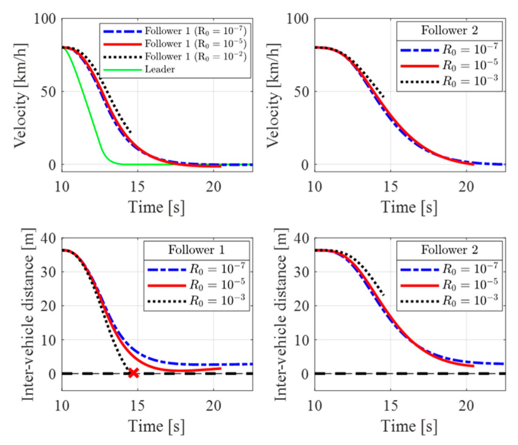
In this scenario, the truck platoon travels at 80 km/h when the leader vehicle suddenly brakes on a high road friction condition. Tests were performed to analyse the performance of the platooning control system with different control calibrations during an emergency braking manoeuvre. The test cases are the same as in Table 1. The simulation stops when the first collision is reached (i.e., when a distance curve crosses the zero line).
Figure 7 shows the results of vehicle velocities (top) and inter-vehicle distance (bottom) during the emergency braking test for different values of R 0 (for both followers): The time headway set of 1.5 s represents the most challenging condition. As seen during the driving cycle, the highest value of ( R 0 = 10 3 ) leads to the greatest inter-vehicle distance error, thus leading to a rear-end collision between follower 1 and the lead vehicle (the impact occurs at ~ 22 km/h). For R 0 = 10 5 and R 0 = 10 7 both vehicles (follower 1 and follower 2) can stop safely (red line).
Figure 8 shows the beneficial effect of higher time headway on safety since for t h = 3   s and t h = 4.5   s the vehicles stop without any collisions (at the same speed the inter-vehicle distance increases) if meanwhile R 0 = 10 5 .
Table 2 summarizes the results of the sensitivity analysis. To avoid the collision, the value of R 0 should be set as low as possible (in fact, for R 0 = 10 3 the follower 1 vehicle collides with the leader for all the analysed time headways) and the time headway the highest possible (but a low time headway is required to increase road capacity). All the computed acceleration and jerk values are well below the comfort limits for the tested driving cycle.
Table 2. Summary of comfort and safety analysis: RMS of jerk and longitudinal acceleration for the driving cycle under investigation. For a quick evaluation of the results, a colormap from green (lowest values) to red (highest value) is adopted to colour the table cells.
Driving Cycle Jerk   [ m / s 3 ] (Limit 0.9 m/s3) a x   [ m / s 2 ] (Limit 2 m/s2)
Vehicle t h   =   1.5   s t h   =   3   s t h   =   4.5   s t h   =   1.5   s t h   =   3   s t h   =   4.5   s
Follower 1 R 0 = 10 7 0.1560.1130.0880.490.4230.373
R 0 = 10 5 0.1540.1110.0860.4950.4280.374
R 0 = 10 3 0.1480.1060.0820.5050.4310.374
Follower 2 R 0 = 10 7 0.1220.0730.0490.4520.360.294
R 0 = 10 5 0.1170.0700.0470.4530.3590.293
R 0 = 10 3 0.1080.0630.0420.4560.3540.287
Given that for R 0 > 10 5 the safety requirement is satisfied for all the time headway values, R 0 = 10 5 has been selected for the comparison with the RL control. The final calibration for the matrices Q and R is:
Q = d i a g 100 ,   10 5 , 100 ,   10 5 ,   20 ,   20
R = d i a g 10 5 , 10 5

4. RL Control System

4.1. Reinforcement Learning for Control

Reinforcement learning is a branch of machine learning with ample application to control systems. It differs both from supervised learning, since it does not require labelled data given from an external supervisor to learn from, and from unsupervised learning, since it attempts to maximise a reward signal rather than trying to find hidden structure in unlabelled data. In essence, reinforcement learning attempts to learn how to map observations to actions that maximise the cumulative reward in the long run [27].
Compared to a more classical approach to control systems, reinforcement learning-based control attempts to compound all functions of a control system (such as state estimation and multiple high- and low-level control loops) into a single agent. The agent interacts with an environment by taking actions a and receiving observations of the states s. When deployed, the agent uses a control policy to decide which actions should be taken as a function of the current observations, and the reinforcement learning algorithm is used in the training phase to train this policy (i.e., tune its parameters) to attain the desired behaviour. More specifically, while training, the agent attempts to maximise the cumulative reward in the long run; hence, the definition of the instantaneous reward is crucial in developing a reinforcement learning agent. The learning procedure does not require an external supervisor to label what the correct action will be. The agent itself must, in fact, identify the latter through a trial-and-error procedure and by interacting with the environment.
Formally speaking, the policy is often described as a mapping π :   S A , where the state space S and the action space A define the (discrete or continuous) sets of possible states and actions. At each time step t , the agent receives the observation s t and takes an action a t . Consequently, it receives from the environment the instantaneous reward r t and the new state s t + 1 . The cumulative reward R = t γ t r t , which the RL algorithm attempts to maximize, is a discounted sum of the instantaneous rewards ( γ [ 0 ,   1 ] being the discount factor). The discounted sum is adopted to transform what would otherwise be an infinite-horizon optimisation problem into a finite-horizon one (there are also other reasons for discounting, such as not using predicted rewards that are too far in the future to be reliable).
The exact structure and representation of the policy, the learning process itself, whether the learning process can take place after deployment or not, and whether the agent can exploit a model of the environment are all defined by the chosen reinforcement learning algorithm. The control designer must hence select the RL algorithm that better suits the application at hand, define a reward function that enforces the desired control objectives, train the algorithm (typically in a simulation environment), and finally test and deploy the agent.
In this work, the chosen algorithm is the deep deterministic policy gradient (DDPG) [28], which is a model-free algorithm whose main features are discussed in Section 4.2. The definition of the reward function as well as the observation and action spaces are reported in Section 4.3.

4.2. The DDPG Algorithm

DDPG is a model-free, off-policy algorithm, meaning that the training phase takes place entirely before deployment and testing. A DDPG agent is also an actor–critic agent, as opposed to a value-based or a policy-based agent. In essence, this means that two different types of function approximators exist.
  • Actor, which receives observations and returns actions (thus playing the role of the policy).
  • The critic, which receives the observations and the actions taken by the actor, evaluates them and returns a prediction of the discounted long-term reward.
During training, the actor’s parameters are updated using the information given by the critic, and the critic itself is updated using the actual rewards received from the environment.
DDPG uses four function approximators: an actor, a critic, a target actor, and a target critic, all four of which are modelled using feed-forward neural networks.
The presence of a target actor and a target critic is a feature that was introduced to improve the stability of the learning process [28]. The target actor and critic networks (which are used when the agent is deployed) are periodically updated using the parameters of the actor and critic using a smoothing technique.
More in detail, we can define a target actor μ t , a target critic Q t , an actor μ and a critic Q . The weights of the target networks θ μ t   and θ Q t   are at first initialized to the weights of the actor and critic networks θ μ and θ Q . Then, they are updated at every time step as follows:
θ μ t   = S F θ μ + 1 S F θ μ t
θ Q t   = S F θ Q + 1 S F θ Q t
where S F is a smoothing factor. In our work, this was set to S F = 10 3 . Furthermore, for all networks, we used three hidden layers with 56 neurons each and used the rectified linear unit (ReLu) as the activation function. The hidden layers and neurons are selected from previous work [29] and adapted to the platoon control problem by increasing the number of layers.
Another notable feature of DDPG is that, since it is an actor–critic network using neural networks as function approximators, it can deal with continuous action and observation spaces that can be either continuous or discrete. This contrasts with other RL methods such as Q-learning, which can only deal with problems in which the action-value function can be represented as a table and where state and action spaces need to be small enough.
Another significant feature of the DDPG algorithm is the experience replay memory, where the data needed for the update process of the parameters of the neural networks during training is stored. At each time step, the memory of the chosen capacity N receives and stores an array containing the current state s , the current action a , the obtained reward r , and the state of the environment after the action. For every training iteration, a batch of n random arrays is sampled from the replay memory and is used to train the critic and actor networks through the respective loss functions L c and L a :
L c = 1 n i = 1 n y Q s , a θ Q 2
L a = 1 n i = 1 n Q s , μ s
In machine learning applications, the amplitude of the step moving towards the minimum of the loss function is called the learning rate. It is one of the main hyperparameter, and in this work it is set to 5 10 5 for the actor network and to 10 4 for the critic one. The capacity of the experience replay memory is set to N = 10 6 . Furthermore, the sample time is set to 0.1 s, since it is small enough to correctly track the lead and depict the energetic aspects. It is typical to use, for this application, a sample time between 0.05 s and 0.2 s [30].
Finally, all reinforcement learning applications require the definition of the training process by controlling the balance between exploration and exploitation. Exploitation refers to the agent picking the action that maximises future reward, whereas exploration refers to the agent selecting a random action during the training process. Clearly, if the training process is unbalanced towards exploitation, the agent may converge to a behaviour that is locally optimal, whereas if the process is unbalanced towards exploration, it may never learn at a reasonable rate.
In this work, we used a common approach and characterised the exploration rate as noise through an Ornstein–Uhlenbeck (OU) action noise model. The default noise mean value is set to 0. It is important to set its standard deviation appropriately to encourage exploration, and for continuous action problems, it is common to set it proportional to the action range [31]. At the same time, the noise standard deviation can be reduced over time to push the algorithm towards exploitation. Such a result can be achieved by introducing a decay rate for the standard deviation, which we set to 10 5 .
The general framework of the DDPG algorithm is shown in Algorithm 1.
Algorithm 1: DDPG Algorithm
1:
Select the driving cycle of the Lead vehicle
2:
Randomly initialize critic and actor network parameters
3:
Initialize experience replay memory with capacity N
4:
Initialize target networks
5:
for episode = 1 to Emax do
6:
Receive initial state
7:
for j = 1 to length of the driving cycle time vector do
8:
Output action from the actor network and add a OU noise for action exploration
9:
Execute   action   a j and observe reward r j , new state s j + 1 from the vehicle model
10:
Store array ( s j , a j , r j , s j + 1 ) in the replay memory
11:
Sample a random minibatch of n arrays from the replay memory
12:
Update critic networks parameters by minimizing L c
13:
Update actor networks parameters by minimizing L a
14:
Update the target networks parameters
15:
end for
16:
end for

4.3. Agent Structure

The objective of the agent is to simultaneously control the whole platoon of vehicles, as the LQC described in the previous section does. Therefore, the agent receives observations from all vehicles and can communicate actions to the two follower vehicles.
In particular, the state vector is defined as follows:
s = t h , 1 t h , 2 v L v F 1 v F 2 a L ,
where:
  • t h , 1 and t h , 2 are the time headway of follower 1 with respect to the leader and follower 2 with respect to follower 1, respectively;
  • v L and a L are the velocity and acceleration of the leader;
  • v F 1 and v F 2 are the velocities of follower 1 and follower 2.
The action vector a is defined by the normalised torque commands for the two follower vehicles, T m , F , 1 and T m , F , 2 :
a = T m , F , 1 T m , F , 2 .
Each normalised torque can range from −1 to 1, with −1 representing the maximum breaking torque and 1 representing the maximum traction torque.
The design of the reward function for the RL controller plays a similar role to the definition of the cost function for the LQC controller that was described in Section 3.2, and a proper definition must be developed to meet the safety and comfort requirements.
In contrast with the LQC cost function, which must be quadratic, there is no restriction on the structure of the reward function. However, to quantitatively compare the performance of the two methods, we decided to express two reward terms, r t h , 1 and r t h , 2 as a quadratic function of the difference between a desired time headway and the current time headway for the two vehicles. The reward was then set to the average of these two terms:
r t h , 1 = 1 w 1 t h , d e s t h , 1 2 , r t h , 2 = 1 w 2 t h , d e s t h , 2 2 ,
r = r t h , 1 + r t h , 2 2 ,
where t h , d e s is the desired time headway and w 1 , w 2 are tuneable weights. Since w 1 and w 2 determine how strictly the agent attempts to enforce the desired time headway of the two followers, in agreement with the LQC approach (where the corresponding elements on the main diagonal of Q and R matrices are the same), they are both set equal to 1.
To guarantee safety and no collision between the vehicles, the following actions are taken if the time headway becomes null:
-
The reward is set to the maximum negative value (−10);
-
The corresponding training iteration has been stopped.

4.4. Evaluation of the RL Agent

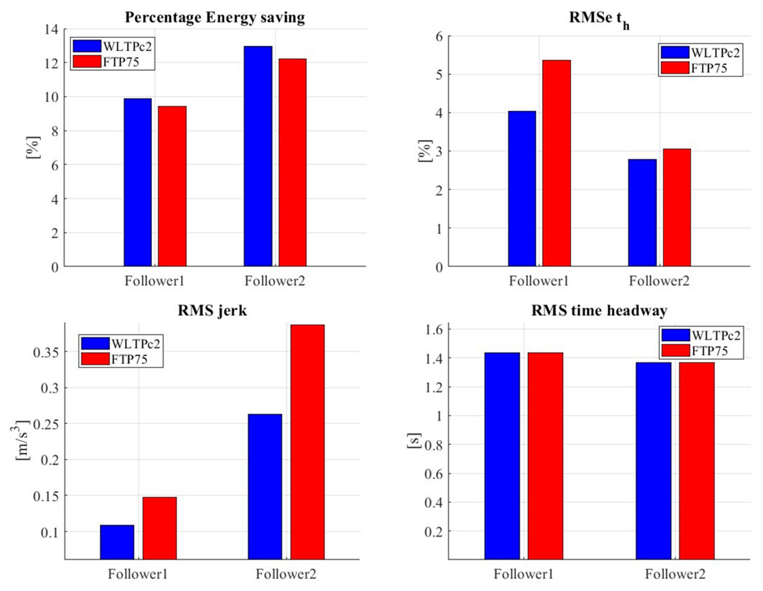
Having set up the agent and the environment as described in the previous sections, the agent was trained using the FTP75 driving cycle as the reference cycle for the leader. Results in Figure 9 show how the agent’s average reward increases during the training, thus showing its learning capacity. The effectiveness of the RL agent was then assessed by testing it on a different driving cycle, i.e., WLTP Class 2.
The results in Figure 10 show the velocities and time gaps of each vehicle for the WLTP driving cycles. The second follower vehicle shows smaller time headway variations with respect to the first follower. Still, they both correctly reproduce the velocity profile of their leading vehicle.
Figure 11 presents a comparison of the following quantities over the training and test cycles for Followers 1 and 2:
  • percentage energy savings with respect to the leader vehicle,
  • RMS of time headway,
  • RMS of time headway error with the desired one
  • RMS of jerk.
The results show that the agent performs even better on the WLTP than on the FTP75 in terms of energy consumption and comfort, with an RMS of time headway that stays almost constant from one driving cycle to the next. Such behaviour can be explained as follows: the agent learns well to generalise over different driving cycles, and the testing cycle turns out to be less demanding in terms of velocity and acceleration, thus allowing both higher energy savings and comfort. Moreover, in this case, for the second follower vehicle, the decreased error on the time headway corresponds to an increase in RMS jerk.

5. Results

In this section, a comparison between the LQ and the RL-based controllers applied to a vehicle platoon composed of one leader and two followers is proposed. Firstly, a discussing about the string stability is provided, then the simulation of two driving situations, to assess the performance of the two controllers, is shown.
-
Standard driving cycle: the leader vehicle tracks the FTP75 driving cycle (saturated to a minimum speed value of 2 m/s to avoid backward movement of the platoon), and the followers try to keep the reference inter-vehicle distance defined by a linear spacing policy and a reference platoon velocity.
-
Cut-in scenario: a new vehicle (not belonging to the platoon) invades the lane occupied by the platoon, thus altering the equilibrium of the controlled system. The controller’s ability to react when an unexpected obstacle breaks the platoon’s equilibrium can therefore be verified.
The followers are controlled by a centralised platooning controller (either LQC- or RL-based) to keep an inter-vehicular distance that depends on the actual vehicle speed (according to a constant-time headway spacing policy). The vehicles forming the platoon are heavy-duty battery electric vehicles with a single-speed transmission and a total mass of 13 tons. The truck data and the parameters of the controllers are available in Table 3; the road slope is assumed to be null ( p = 0 ). The LQ and RL-based controllers are tested in the same framework, consisting of the driving scenario and the nonlinear vehicle platoon model described in Section 2.

5.1. String Stability

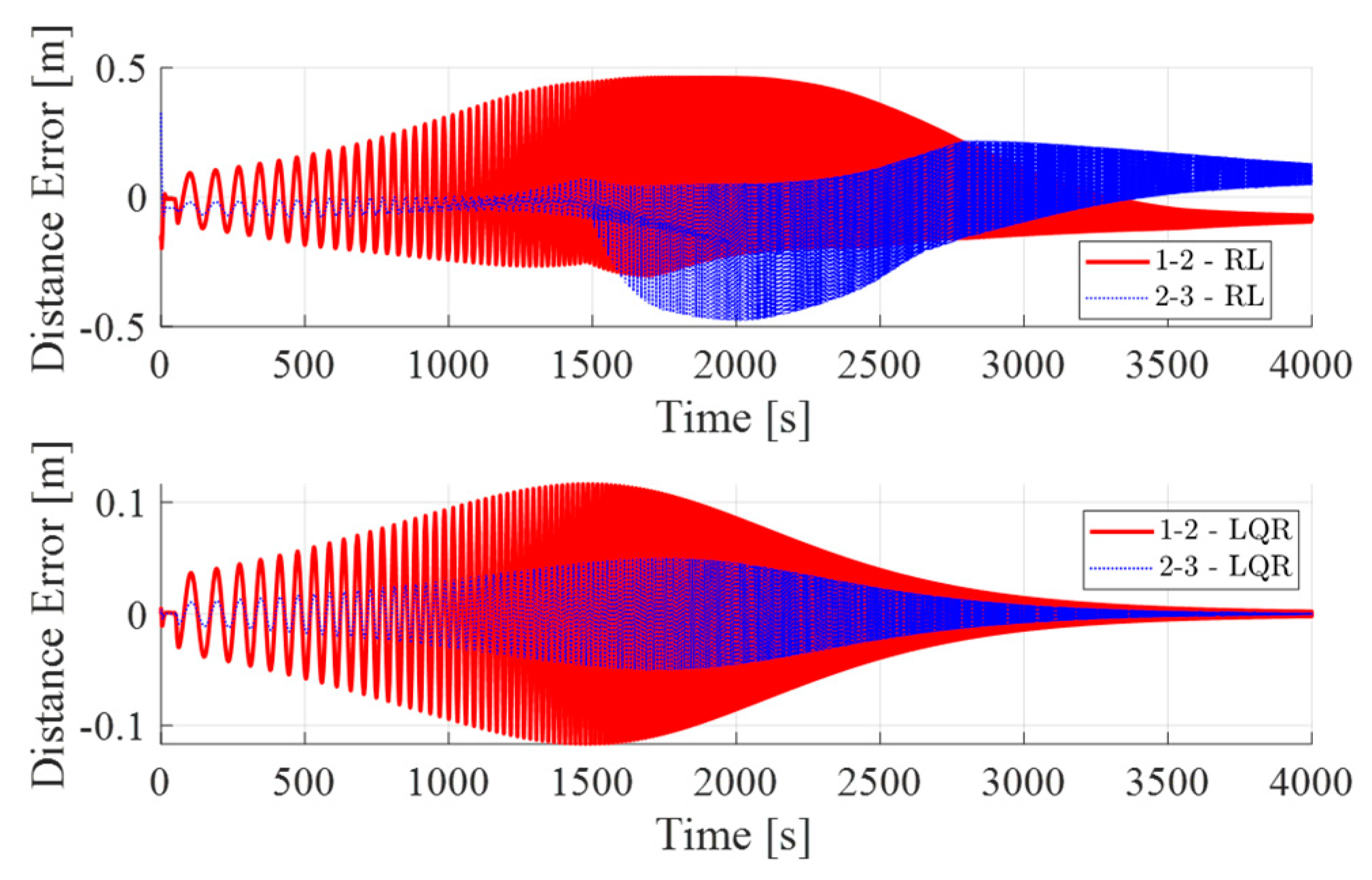
Platoon systems can show string stability issues. It represents a safety concern since a string stable platoon allows to avoid traffic collisions and traffic jams when a long string of vehicles travels along the same route. This evidence is investigated by different literature works, both experimentally and numerically. In particular, the methodology for the assessment of the platoon string stability is described in [11], which states that the sufficient condition to guarantee platoon string stability is:
| H j ω | < 1
where:
H j ω = E d , 23 j ω E d , 12 ( j ω )
representing the frequency response function of two consecutive distance errors E d , 23 and E d , 12 , which account for the propagation of perturbances along the platoon. Thus, the string stability is verified by testing the LQC and RL performance by exciting the platoon dynamics with a sine sweep disturbance applied by the lead vehicle velocity. The frequency range is set from 10 4 to 5 Hz. The test is carried out at 40 km/h, and the amplitude of the lead vehicle speed disturbance is set to 1.5 km/h. The results in the time domain of the error distances ( e d 1,2 , e d 2,3 ) are reported in Figure 12 for both controllers. The string stability condition is satisfied when the amplitude of e d 2,3 (blue line) is less than e d 1,2 (red line). The LQC is string-stable across the entire frequency range. On the other hand, the RL-based controller ensures a bandwidth of string stability of 0 0.3   H z . In fact, as can be noted from the time history (top part of Figure 12), the blue line shows an amplitude of oscillation smaller than the red one until 2800   s (when the corresponding frequency is f ~ 0.3   H z ) . Nevertheless, this range is compliant with the typical longitudinal dynamics control of heavy-duty trucks, e.g., the frequency range investigated in [11], and was therefore considered satisfactory.
Moreover, differently from the LQC, the RL signals are clearly affected by nonlinearities; in fact, the frequency content of the signals includes both fundamental harmonics due to the frequency of the excitation and super-harmonics (see spectrograms in Figure 13) because of control nonlinearity. This control-related nonlinear behaviour comes from the combined operation of the safety-related penalty on the reward function and the activation functions of the neural network.

5.2. LQC—RL Comparison

5.2.1. Driving Cycle Results

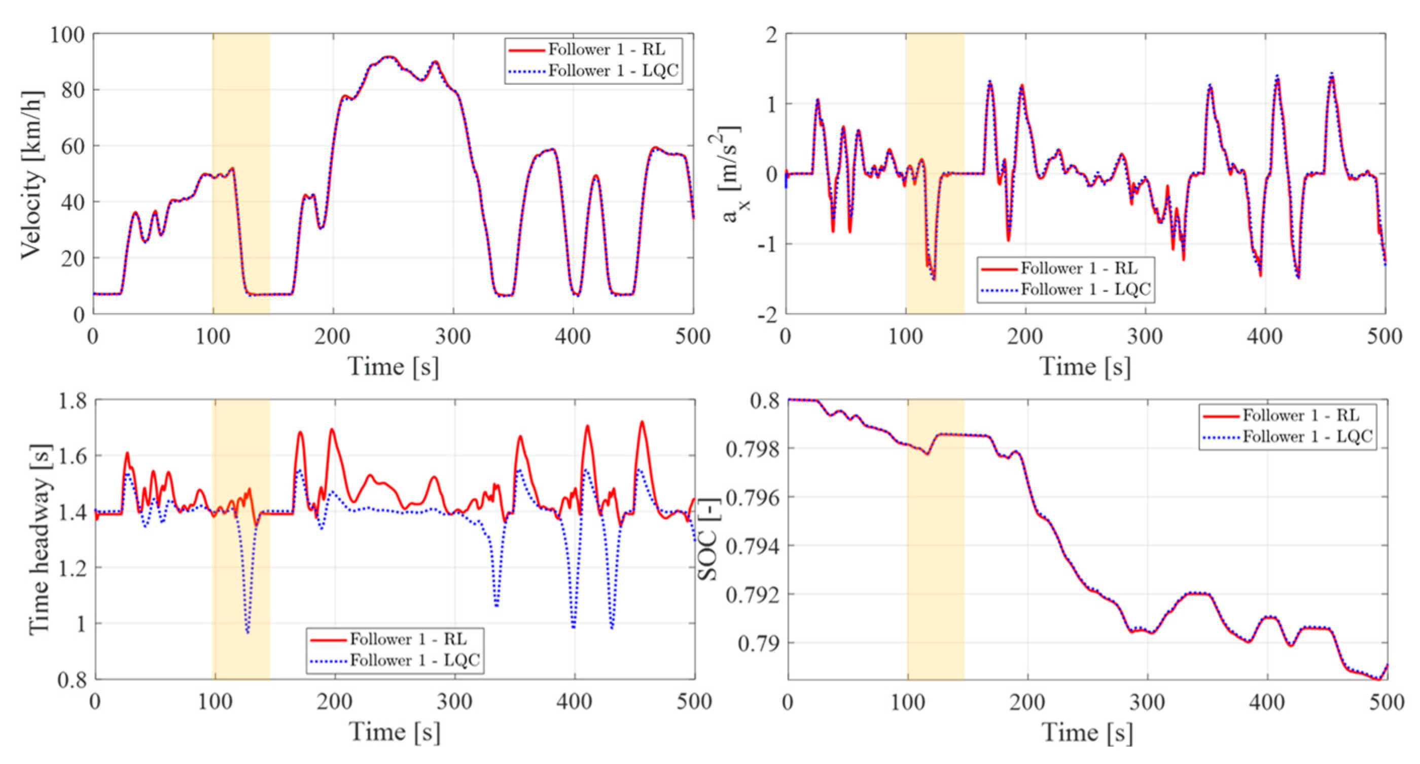
For the sake of visibility, in Figure 14, the comparison of the two controllers over the first follower vehicle is represented. As clearly shown by the figure, the controllers achieve almost identical speed profiles. The small differences in vehicle accelerations cause a clearer difference in time headway, especially during braking.
With reference to the highlighted area where the platoon is braking, it can be observed that, while LQC’s actual time headway is lower than the target one, RL has the opposite trend, i.e., the actual value is greater. This difference can be justified by the asymmetry of the RL control due to the penalty introduced in the reward function to avoid collisions during braking.
Consequently, also from an energetic standpoint, the results are comparable since the state of charge profiles of the two simulations overlap (see the SOC trends reported in Figure 14).
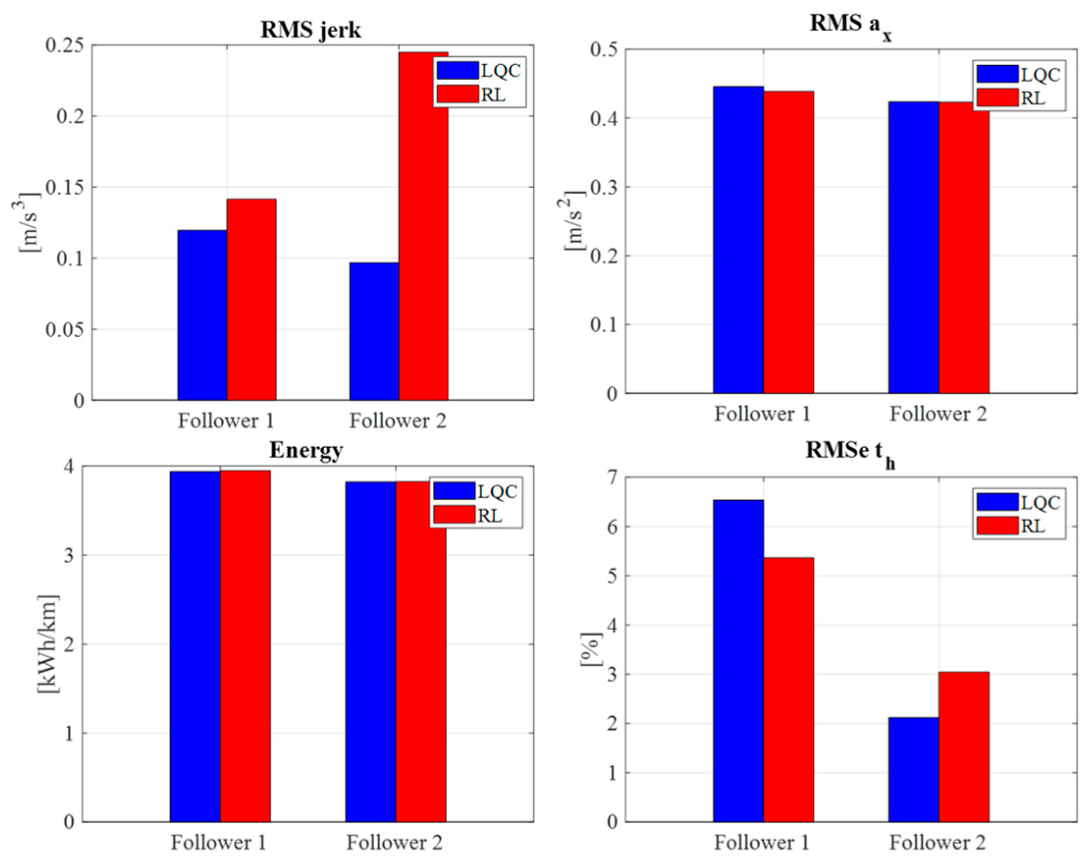
Figure 15 shows the results of the performance indices introduced to evaluate the drivability (RMS jerk and longitudinal acceleration), the energy consumption, and the controller performance (RMSE of the time headway).
The RMSE of time headway reduces from the first to the second follower for both the controllers, but the reduction is stronger for the LQC case, where the error passes from 6 to 2% and RL from 5.5% to 3%.
As for the energy consumption of the first follower, the difference between the two controllers is less than 3%, respectively, 3.93 kWh/km (RL) and 3.83 kWh/km (LQC). From the comparison in terms of comfort, RL shows a lower RMS of acceleration but a higher jerk. Moreover, the jerk along the string increases for the RL, while it decreases for the LQC. However, the increase in the RMS of jerk results in comfortable driving because the values remain within the limit previously defined.

5.2.2. Cut-In Scenario Results

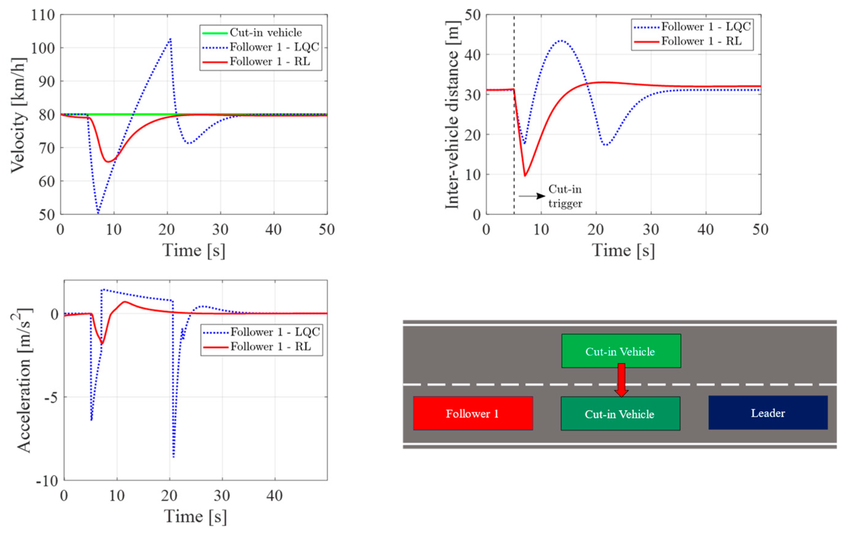
In this scenario, the truck platoon is travelling at 80 km/h on a highway road when a vehicle suddenly breaks the platoon lane. Figure 16 shows an example of the investigated scenario: the green vehicle performs a cut-in manoeuvre in the platoon lane, between the leader and the follower 1 truck. In the simulation, the cut-in vehicle behaviour is modelled through a linear variation in 2 s of the leader position while maintaining its initial velocity (80 km/h). The cut-in vehicle’s final position is set to split equally the available space between the vehicles. The cut-in vehicle is assumed to be a truck with the same inertial and geometrical characteristics listed in Table 3. Figure 16 depicts the simulation results of the two controllers in terms of velocity profile, inter-vehicle distance, and longitudinal acceleration for the driving cycle. The solid green line represents the velocity of the cut-in vehicle, and the dashed black line represents the event that triggers the cut-in manoeuvre. Both the controllers properly reduce the vehicle speed when the disturbance occurs, but the LQC guarantees a minimum distance error that is half of the RL one, thus improving the platoon’s safety under critical conditions. The LQC applies a braking torque higher than the RL one, thus resulting in a higher longitudinal acceleration. Such behaviour stems from the innate difference between the two algorithms. The RL controller has learned a smoother approach that allows for reaching lower distances during the cut-in, thus achieving greater comfort. On the contrary, LQC tries to maximise performance in terms of safety. However, both controllers proved to be able to reduce the distance error, and they reached the reference distance (33 m) at steady state. The LQC results in more aggressive behaviour, i.e., it brakes twice to obtain the reference distance.

6. Conclusions

In this paper, a collaborative centralised platooning control system has been obtained through two different control techniques, i.e., the linear quadratic controller and the reinforcement learning-based controller.
The main outcomes of this research activity are:
  • The proposed model of the truck platoon includes the dependency of the aerodynamic drag with the inter-vehicle distance; it is vital to quantify the fuel savings of each vehicle in the platoon.
  • The virtual environment that has been developed enables one to tune and train classical and AI controllers and assess platoon performance under different driving cycles.
  • The LQC controller is string stable across the entire frequency range, while the RL-based controller may have a limited bandwidth of string stability.
  • Regardless of the type of controller, a linear spacing policy proved to be a suitable choice to meet all the requirements (dynamic performance and energy savings).
  • The training of RL provides satisfactory results even in the case of driving cycles different from the ones used for the learning phase of the agent.
  • The simulation results of an RL-based controller are affected by nonlinearities; this control-related nonlinear behaviour comes from the combined operation of the safety-related penalty on the reward function and the activation functions of the neural network.
  • The comparison through the selected performance indices (i.e., acceleration and jerk, final SOC, and energy consumption) during a standard driving cycle showed that, by properly selecting the reward function, RL and LQC achieve similar dynamic and energetic targets.
  • The comparison during a cut-in simulation scenario showed that both controllers properly reduced the vehicle speed when the disturbance occurred, avoiding accidents.

Author Contributions

Methodology, A.B., L.Z., F.M., E.G., D.A.M. and A.T.; Software, A.B. and L.Z.; Writing—original draft, A.B. and L.Z.; Writing—review & editing, F.M., E.G. and D.A.M.; Supervision, E.G. and D.A.M.; Project administration, E.G. and D.A.M. All authors have read and agreed to the published version of the manuscript.

Funding

This research received no external funding.

Institutional Review Board Statement

Not applicable.

Informed Consent Statement

Not applicable.

Data Availability Statement

Not applicable.

Conflicts of Interest

The authors declare no conflict of interest.

Appendix A

The coefficients of the Equations (8) and (12) are:
A 0 = m g A 1 = m g f 0 B 0 = m g f 2 B 1 = 1 2 ρ A f
K i = A 1 + B 0 + B 1 c x , i d n v n m i , t o t G i = 2 B 0 + B 1 F 1 v n m i , t o t E i = A 0 α n m i , t o t v n S i = B 1 F 2 v n m i , t o t
where the coefficients F 1 and F 2 depends by the linearisation of the Equation (5):
F 1 = a 2 d n 2 + a 1 d n + a 0 b 2 d n 2 + b 1 d n + b 0
F 2 = a 0 a 1 a 1 b 0 d n + a 0 b 2 a 2 b 0 2 d n 2 + a 1 b 2 a 2 b 1 d n 3 ( b 2 d n 2 + b 1 d n + b 0 ) ^ 2
Considering a platoon of three vehicles, the matrices of the state-space system are:
[ A ] = 0 v n d n 0 0 0 0 S 2 G 2 0 0 0 0 0 v n d n 0 v n d n 0 0 0 0 S 3 G 3 0 0 1 0 0 0 0 0 0 0 1 0 0 0 ;
[ B ] = 0 0 K 2 0 0 0 0 K 3 0 0 0 0
H = 0 0 E 1 0 0 0 0 E 2 0 0 0 0 ; C = v n d n   0   0   0   0   0   ;

Appendix B

B + is the pseudoinverse of matrix B if and only if all the following conditions 1 ( 4 ) are satisfied:
  • B B + B = B
  • B + B B + = B +
  • B B + T = B B +
  • B + B T = B + B

References

  1. Alam, A.; Gattami, A.; Johansson, K.H.; Tomlin, C.J. Guaranteeing safety for heavy duty vehicle platooning: Safe set computations and experimental evaluations. Control. Eng. Pr. 2014, 24, 33–41. [Google Scholar] [CrossRef]
  2. Vahidi, A.; Sciarretta, A. Energy saving potentials of connected and automated vehicles. Transp. Res. Part C Emerg. Technol. 2018, 95, 822–843. [Google Scholar] [CrossRef]
  3. Tsugawa, S.; Jeschke, S.; Shladovers, S.E. A review of truck platooning projects for energy savings. IEEE Trans. Intell. Veh. 2016, 1, 68–77. [Google Scholar] [CrossRef]
  4. Bergenhem, C.; Pettersson, H.; Coelingh, E.; Englund, C.; Shladover, S.; Tsugawa, S. Overview of platooning systems. In Proceedings of the 19th ITS World Congress, Vienna, Austria, 22–26 October 2012. [Google Scholar]
  5. Ellis, M.; Gargoloff, J.I.; Sengupta, R. Aerodynamic Drag and Engine Cooling Effects on Class 8 Trucks in Platooning Configurations. SAE Int. J. Commer. Veh. 2015, 8, 732–739. [Google Scholar] [CrossRef]
  6. Kaluva, S.T.; Pathak, A.; Ongel, A. Aerodynamic drag analysis of autonomous electric vehicle platoons. Energies 2020, 13, 4028. [Google Scholar] [CrossRef]
  7. McAuliffe, B.; Lammert, M.; Lu, X.Y.; Shladover, S.; Surcel, M.D.; Kailas, A. Influences on Energy Savings of Heavy Trucks Using Cooperative Adaptive Cruise Control. In SAE Technical Papers; SAE International: Warrendale, PA, USA, 2018. [Google Scholar] [CrossRef]
  8. Zhang, R.; Li, K.; Wu, Y.; Zhao, D.; Lv, Z.; Li, F.; Chen, X.; Qiu, Z.; Yu, F. A Multi-Vehicle Longitudinal Trajectory Collision Avoidance Strategy Using AEBS with Vehicle-Infrastructure Communication. IEEE Trans. Veh. Technol. 2022, 71, 1253–1266. [Google Scholar] [CrossRef]
  9. Wu, C.; Xu, Z.; Liu, Y.; Fu, C.; Li, K.; Hu, M. Spacing policies for adaptive cruise control: A survey. IEEE Access 2020, 8, 50149–50162. [Google Scholar] [CrossRef]
  10. Gunter, G.; Gloudemans, D.; Stern, R.E.; McQuade, S.; Bhadani, R.; Bunting, M.; Monache, M.L.D.; Lysecky, R.; Seibold, B.; Sprinkle, J.; et al. Are Commercially Implemented Adaptive Cruise Control Systems String Stable? IEEE Trans. Intell. Transp. Syst. 2021, 22, 6992–7003. [Google Scholar] [CrossRef]
  11. Naus, G.J.L.; Vugts, R.P.A.; Ploeg, J.; Van De Molengraft, M.J.G.; Steinbuch, M. String-stable CACC design and experimental validation: A frequency-domain approach. IEEE Trans. Veh. Technol. 2010, 59, 4268–4279. [Google Scholar] [CrossRef]
  12. Besselink, B.; Johansson, K.H. String Stability and a Delay-Based Spacing Policy for Vehicle Platoons Subject to Disturbances. IEEE Trans. Autom. Control 2017, 62, 4376–4391. [Google Scholar] [CrossRef]
  13. Sugimachi, T.; Fukao, T.; Suzuki, Y.; Kawashima, H. Development of autonomous platooning system for heavy-duty trucks? In IFAC Proceedings Volumes (IFAC-PapersOnline); IFAC Secretariat: Laxenburg, Austria, 2013; pp. 52–57. [Google Scholar] [CrossRef]
  14. Turri, V.; Besselink, B.; Johansson, K.H. Cooperative Look-Ahead Control for Fuel-Efficient and Safe Heavy-Duty Vehicle Platooning. IEEE Trans. Control Syst. Technol. 2017, 25, 12–28. [Google Scholar] [CrossRef]
  15. Ward, J.W.; Stegner, E.M.; Hoffman, M.A.; Bevly, D.M. A Method of Optimal Control for Class 8 Vehicle Platoons Over Hilly Terrain. J. Dyn. Syst. Meas. Control 2022, 144, 011108. [Google Scholar] [CrossRef]
  16. Gao, W.; Gao, J.; Ozbay, K.; Jiang, Z.P. Reinforcement-Learning-Based Cooperative Adaptive Cruise Control of Buses in the Lincoln Tunnel Corridor with Time-Varying Topology. IEEE Trans. Intell. Transp. Syst. 2019, 20, 3796–3805. [Google Scholar] [CrossRef]
  17. Yang, J.; Liu, X.; Liu, S.; Chu, D.; Lu, L.; Wu, C. Longitudinal tracking control of vehicle platooning using DDPG-based PID. In Proceedings of the 2020 4th CAA International Conference on Vehicular Control and Intelligence, CVCI 2020, Hangzhou, China, 18–20 December 2020; Institute of Electrical and Electronics Engineers Inc.: Piscataway, NJ, USA, 2020; pp. 656–661. [Google Scholar] [CrossRef]
  18. Peake, A.; McCalmon, J.; Raiford, B.; Liu, T.; Alqahtani, S. Multi-Agent Reinforcement Learning for Cooperative Adaptive Cruise Control. In Proceedings of the International Conference on Tools with Artificial Intelligence, ICTAI, Baltimore, MD, USA, 9–11 November 2020; IEEE Computer Society: Washington, DC, USA, 2020; pp. 15–22. [Google Scholar] [CrossRef]
  19. Chu, T.; Kalabić, U. Model-based deep reinforcement learning for CACC in mixed-autonomy vehicle platoon. In Proceedings of the 2019 IEEE 58th Conference on Decision and Control (CDC), Nice, France, 11–13 December 2019; pp. 4079–4084. [Google Scholar] [CrossRef]
  20. Lin, Y.; McPhee, J.; Azad, N.L. Comparison of Deep Reinforcement Learning and Model Predictive Control for Adaptive Cruise Control. IEEE Trans. Intell. Veh. 2021, 6, 221–231. [Google Scholar] [CrossRef]
  21. Hussein, A.A.; Rakha, H.A. Vehicle Platooning Impact on Drag Coefficients and Energy/Fuel Saving Implications. IEEE Trans. Veh. Technol. 2022, 71, 1199–1208. [Google Scholar] [CrossRef]
  22. Vogel, K. A comparison of headway and time to collision as safety indicators. Accid. Anal. Prev. 2003, 35, 427–433. [Google Scholar] [CrossRef]
  23. Ostertag, E. Mono- and Multivariable Control and Estimation: Linear, Quadratic and LMI Methods; Springer Science & Business Media: Berlin, Germany, 2011. [Google Scholar] [CrossRef]
  24. Dimauro, L.; Tota, A.; Galvagno, E.; Velardocchia, M. Torque Allocation of Hybrid Electric Trucks for Drivability and Transient Emissions Reduction. Appl. Sci. 2023, 13, 3704. [Google Scholar] [CrossRef]
  25. Barata, J.C.A.; Hussein, M.S. The Moore-Penrose Pseudoinverse: A Tutorial Review of the Theory. Braz. J. Phys. 2012, 42, 146–165. [Google Scholar] [CrossRef]
  26. Bae, I.; Moon, J.; Jhung, J.; Suk, H.; Kim, T.; Park, H.; Cha, J.; Kim, J.; Kim, D.; Kim, S. Self-Driving like a Human driver instead of a Robocar: Personalized comfortable driving experience for autonomous vehicles. arXiv 2020, arXiv:2001.03908. [Google Scholar]
  27. Sutton, R.S.; Barto, A.G. Reinforcement Learning: An Introduction, 2nd ed.; MIT Press: Cambridge, MA, USA, 2018. [Google Scholar]
  28. Lillicrap, T.P.; Hunt, J.J.; Pritzel, A.; Heess, N.; Erez, T.; Tassa, Y.; Silver, D.; Wierstra, D. Continuous control with deep reinforcement learning. arXiv 2015, arXiv:1509.02971. [Google Scholar]
  29. Acquarone, M.; Borneo, A.; Misul, D.A. Acceleration control strategy for Battery Electric Vehicle based on Deep Reinforcement Learning in V2V driving. In Proceedings of the 2022 IEEE Transportation Electrification Conference & Expo (ITEC), Anaheim, CA, USA, 15–17 June 2022. [Google Scholar]
  30. Wei, S.; Zou, Y.; Zhang, T.; Zhang, X.; Wang, W. Design and experimental validation of a cooperative adaptive cruise control system based on supervised reinforcement learning. Appl. Sci. 2018, 8, 1014. [Google Scholar] [CrossRef]
  31. MATLAB & Simulink—MathWorks Italia. Train DDPG Agent for Adaptive Cruise Contro; MATLAB & Simulink—MathWorks Italia: Torino, Italy, 2023. [Google Scholar]
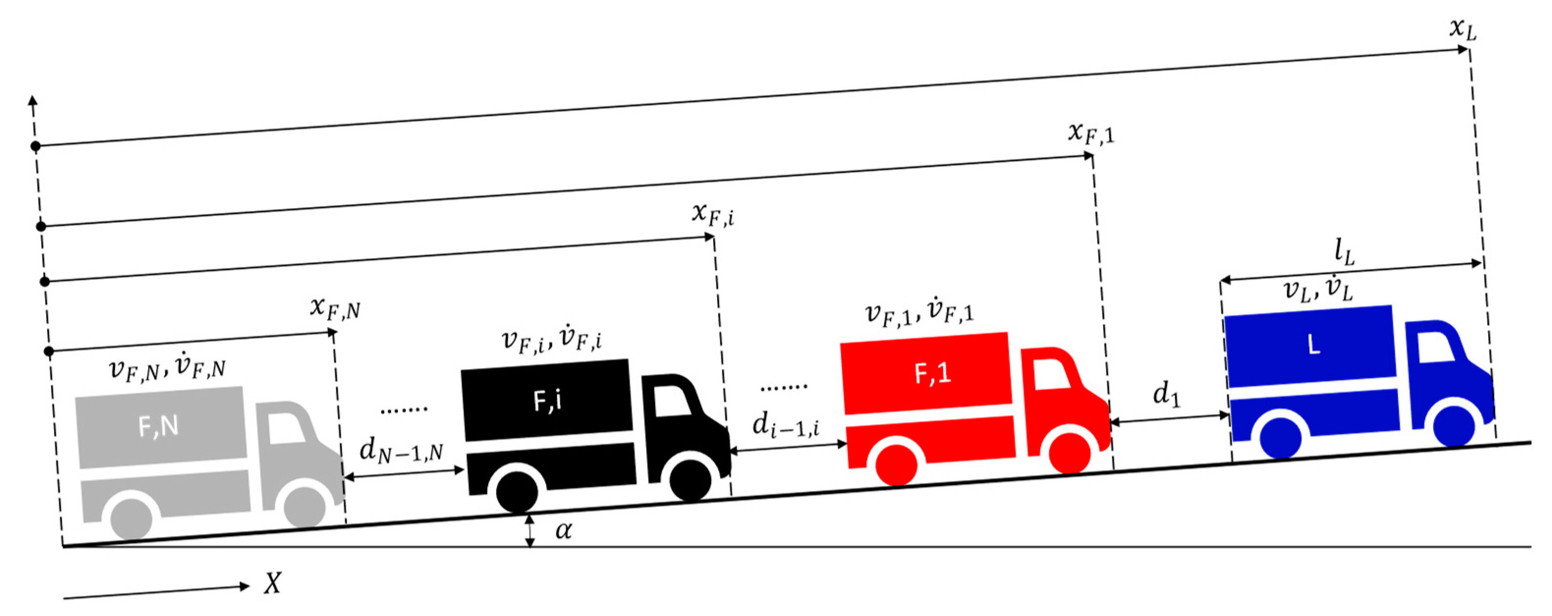
Figure 1. Vehicle platooning on straight and sloped roads.
Applsci 13 10459 g001
Figure 2. Map of drag coefficient dependency on the inter-vehicle distance d .
Applsci 13 10459 g002
Figure 3. Energy consumption comparison between the set of isolated vehicles (left) and the vehicle platoon (right): blue bar is the lead vehicle, red bar the follower 1 and black bar the follower 2.
Applsci 13 10459 g003
Figure 4. Block diagram of the platooning system with LQC.
Applsci 13 10459 g004
Figure 5. WLTP Class 3 simulation with LQC: velocity response, inter-vehicle distance error, and electric motor torque for three different values of R 0 = [ 10 7 , 10 5 , 10 3 ] with t h = 1.5   s .
Applsci 13 10459 g005
Figure 6. WLTP Class 3 simulation with LQC: velocity response, inter-vehicle distance error, electric motor torque, and longitudinal acceleration for three different values of t h = [ 1.5   s , 3   s , 4.5   s ] with R 0 = 10 5 .
Applsci 13 10459 g006
Figure 7. Emergency braking manoeuvre results: follower 1 and follower 2 velocity (top) and inter-vehicle distance (bottom) R 0 = [ 10 7 , 10 5 , 10 3 ] with t h = 1.5   s .
Applsci 13 10459 g007
Figure 8. Emergency braking manoeuvre results: follower 1 and follower 2 velocity (top) and inter-vehicle distance (bottom) t h = 1.5   s , 3   s , 4.5   s with R 0 = 10 5 .
Applsci 13 10459 g008
Figure 9. Average reward for training over the FTP75 cycle.
Applsci 13 10459 g009
Figure 10. Velocity and Time Headway for the testing over the WLTP Class 2 driving cycle.
Applsci 13 10459 g010
Figure 11. Comparison between the WLTP and FTP75 for the RL assessment.
Applsci 13 10459 g011
Figure 12. Distance errors from the two controllers when the platoon is excited by a chirp disturbance: on top the RL distance errors (red line vehicle 1–2, blue line 2–3), on bottom LQC distance errors.
Applsci 13 10459 g012
Figure 13. Spectrograms of the distance errors from the LQC (top) and RL (bottom) during the sine sweep test.
Applsci 13 10459 g013
Figure 14. Results of the comparison of the two controllers during a FPT75 driving cycle: solid red RL results, dotted blue LQC results. The plot refers to the Follower 1 vehicle.
Applsci 13 10459 g014
Figure 15. Comparison of LQC and RL indices: RMS jerk, longitudinal acceleration, energy consumption, and error on time headway.
Applsci 13 10459 g015
Figure 16. Comparison between the LQC and RL during a cut-in scenario simulation: solid red line—RL; dotted blue trace—LQC; green trace (solid and dashed)—cut-in vehicle velocity and distance.
Applsci 13 10459 g016
Table 1. R 0 and t h values used in the sensitivity analysis in the WLTP Class 3 and emergency braking tests.
R 0 t h [ s ]
10 7 1.5 ,   3 ,   4.5
10 5 1.5 ,   3 ,   4.5
10 3 1.5 ,   3 ,   4.5
Table 3. Truck data and platooning controller parameters.
QuantitySymbolValue
Equivalent vehicle mass m t o t i 13,175 kg
Wheel radius r w , i 0.5715 m
Electric motor maximum power P m , m a x   300 kW
Electric motor maximum torque T m , m a x   600 Nm
Total transmission efficiency η 95%
Total transmission ratio τ 19.74
Battery max capacity Q b a t t 693 Ah
Battery Nominal Voltage V b a t t , n 500 V
Initial SOC S O C 0 80%
Isolated vehicles drag coefficient c x , 0 0.57
Air density ρ 1.2
Vehicle frontal Area A f , i 8.9 m 2
Road-tyre friction coefficient μ 0.9
Rolling resistance coefficient f 0 0.0041
Rolling resistance coefficient f 2 0
Time headway t h , d e s 1.4 s
Nominal speed v n 80 km/h
Nominal inter-vehicle distance d n 36 m
Nominal road slope α n
LQC: Q—matrix Q d i a g 10 2 , 10 5 , 10 2 , 10 5 , 20 ,   20
LQC: R—matrix R 10 5 × d i a g 1,1
RL: reward function weight 1 w 1 1
RL: reward function weight 2 w 2 1
RL: Actor learning rate l r a 5 × 10 5
RL: Critic learning rate l r c 10 4
Disclaimer/Publisher’s Note: The statements, opinions and data contained in all publications are solely those of the individual author(s) and contributor(s) and not of MDPI and/or the editor(s). MDPI and/or the editor(s) disclaim responsibility for any injury to people or property resulting from any ideas, methods, instructions or products referred to in the content.