Research and Simulation of Kinematics and Dynamics of Tracked Support Equipment Based on Multi-Body Dynamics

Abstract

Aiming at addressing the problems of low production efficiency and low safety factors in coal mines, this study designed a new type of support equipment and verified its theoretical reliability through the analysis of driving theory. The analysis was carried out through kinematics and dynamics, the position coordinates of the prototype at different times were analyzed using the RPY angles, and the spatial coordinate system of the prototype was established. Then, the position coordinates at different times could be solved by establishing the plane kinematics equations of the prototype. A 14-degree-of-freedom dynamic system model was established to reflect the longitudinal dynamic characteristics of the traveling mechanism of the prototype, and the differential equations of the traveling mechanism were established via the Lagrange dynamic equation method. Finally, the dynamic stability of the prototype under different working conditions was studied by using multi-body dynamic simulation technology. The research results show that the prototype meets the design requirements, has good reliability, realizes the mechanization, automation and high-efficiency production of coal mines, and realizes safe underground production. The research results provide effective solutions for ensuring the sustainable development of coal resources and the safe production of coal mines.

1. Introduction

Given the special position of coal in China’s energy structure, the issue of coal mine safety has always attracted much attention [1,2]. At present, integral hydraulic pillars are widely used in the hollow roof support of thin coal seam driving face roadways and coal mining face roadways. This support method requires manual handling and is characterized by a poor underground working environment, long working time, and low working efficiency. In the process of coal mining, the roof is prone to rock fall and roof collapse, posing a threat to the operators. Meanwhile, the emulsion discharged in the operation pollutes the working face environment [3]. Therefore, the safety of production has always been the top priority in coal mining research. Hou et al. put forward the problems existing in coal mine excavation and support, and put forward suggestions to improve the level of underground equipment and mechanization [4]. Sakhno Ivan et al. studied the in situ deformation process of the surrounding rock of an auger drilling roadway in a roof anchoring system and designed a suitable support system. The results show that the bolt support can be used in auger mining roadway support [5]. Shahzad M et al.’s study focused on the strength characteristics of flexural and compression components of acacia wood used as underground support components in coal mines to evaluate the mechanical characteristics of typical support systems in thin coal seam mining in Pakistan [6]. Xue et al. introduced the development course of mine support equipment from the primary stage to the advanced stage, and pointed out the further development direction of China’s mine support equipment [7]. Li designed a large self-moving support device and studied its mechanical properties through numerical simulation [8]. Luca Bruzzone et al. discussed the latest technology in the motion system of ground mobile robots composed of tracks, and also reviewed the modeling, simulation and design methods of tracked ground mobile robots [9].

Previously, when designing using classical methods, the vehicle is usually assumed to be a rigid solid combination [10,11,12] system, and the motion description generalized coordinates are used, with the solids connected by spring-damped units. At present, most coal mines in China are relatively short of funds and cannot use existing supporting equipment on a large scale [13]. This paper innovatively designs a kind of double movable column hydraulic prop, as shown in Figure 1.

The structural characteristics are mainly reflected in four aspects:

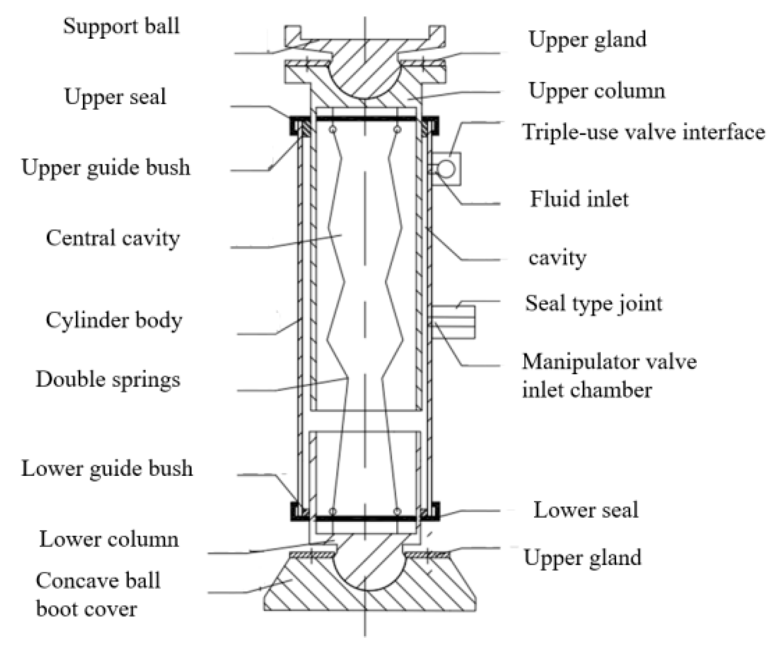
• A double live column design is adopted, and the structure realizes bidirectional live column extension together with the self-transferring traveling mechanism, which improves the supporting efficiency;
• The upper and lower double live columns are designed with a ball-type slewing structure to adapt to the changes in the angle of the bottom plate and top plate of the coal mine underground and ensure the stability of the force of the hydraulic pillar in the support process;
• The cylinder body is welded with self-sealing connecting hose fittings to prevent the air from entering the working chamber of the hydraulic pillar, preventing cavitation and rusting of the system components, thus reducing the maintenance cost and improving the working life of the components, which is in line with the concept of green mine;
• The use of coal mine three-use valves and controllers to realize dual operation and dual control mode improves operation flexibility and efficiency and ensures the safety and reliability of roof support.

Mechanical systems with rigid body dynamics are modeled using methods based on Newton’s laws of motion [14]. However, there are some difficulties in modeling multi-body systems. When more mechanical parts are interconnected, modeling tends to rely on geometry, and simulating these mechanical systems can require considerable effort [15]. Therefore, this paper takes Jisuo Coal mine as an example to study a self-propelled closed-bracket virtual prototype (MSES virtual prototype for short) in a coal mine, as shown in Figure 2 and Figure 3. The MSES virtual prototype is mainly applied to a thin coal seam. Due to the narrow underground space, the prototype designed in this paper is 1.2 m long, 1.1 m wide and 0.5 m high, respectively.

2. Driving Theory Analysis

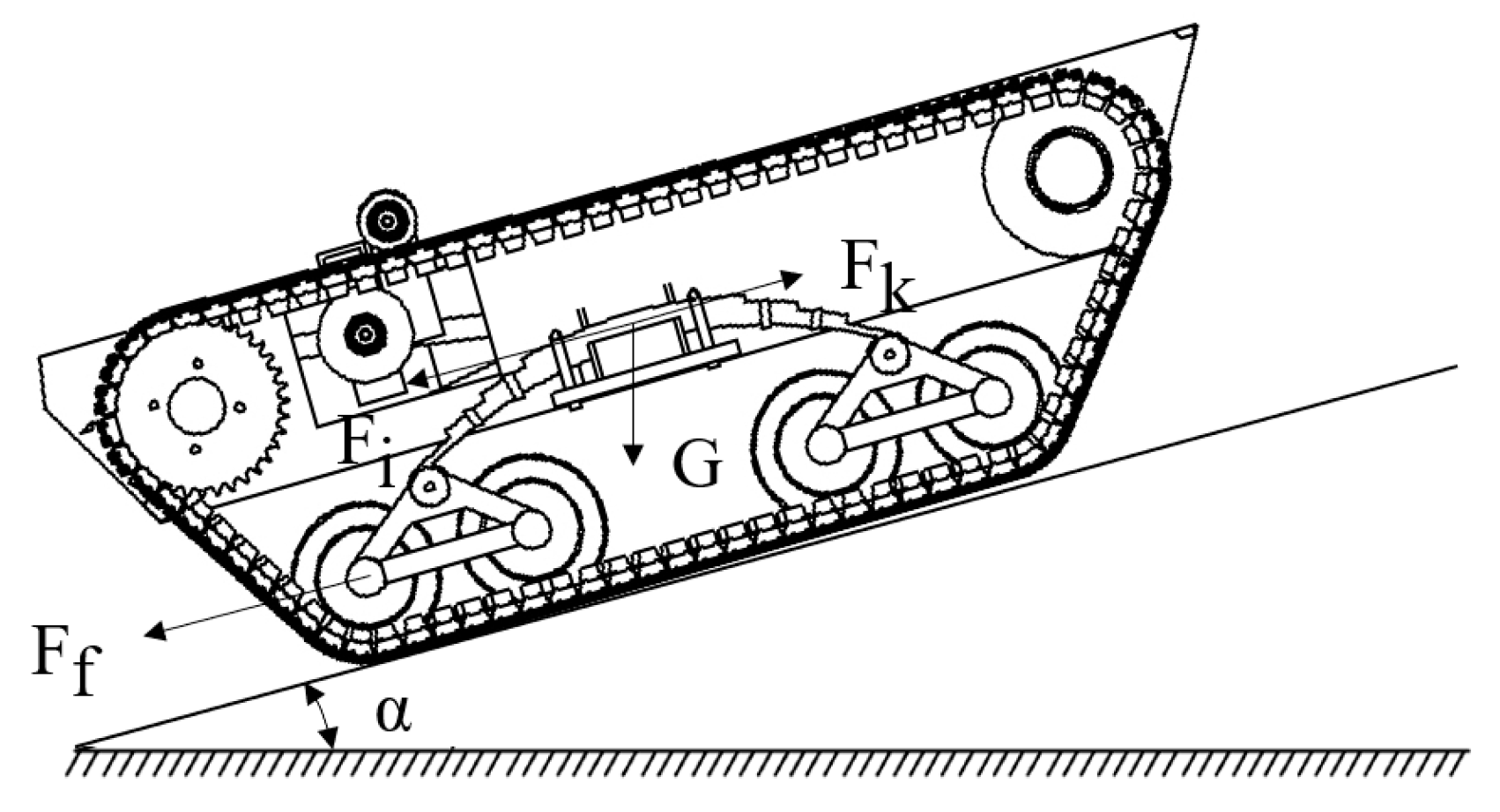
2.1. Driving Resistance Analysis

The prototype needs to overcome rolling resistance, climbing resistance, steering resistance, internal resistance, inertial resistance and air resistance during traveling. Due to its large weight and slow traveling speed, the air resistance can be ignored. The force diagram of the prototype is shown in Figure 4.

When the prototype traveled, the rolling resistance that prevented the movement of the transporter was generated due to the shear deformation of the soil and the internal resistance of the track chassis. Rolling resistance is given by Equation (1):

$$F_f=m\mathrm{g}f\mathit{cos}\alpha$$

(1)

where $m$ is the total mass of the prototype, g is acceleration due to gravity, $f$ is the coefficient of rolling resistance, and $\alpha$ is the angle of the slope.

Climbing resistance refers to the resistance caused by the partial force of gravity in the direction of the slope while traveling up a slope. Climbing resistance is given by Equation (2):

$$F_i=m\mathrm{g}f\sin \alpha$$

(2)

The steering moment of resistance usually consists of two parts, namely the moment of resistance due to friction and the component force of the traction force when steering, and only the first part of the moment of resistance is considered in this paper. Steering resistance is given by Equation (3):

$$F_z=\frac{\mu m\mathrm{g}\mathrm{L}}{4R}$$

(3)

where $\mu$ is the steering resistance coefficient, L is the length of track grounding, and R is the turning radius of the prototype.

Internal resistance generally includes the resistance to engagement between the drive wheel and the track, the friction between the drive wheel and guide wheel journals, the friction between the track pins, and the frictional resistance of the support wheel. Internal resistance is given by Equation (4):

$$F_n=0.03\mathrm{m}\mathrm{g}$$

(4)

Inertial resistance is an inertial force that develops as a result of a change in velocity causing the overall mass to accelerate. Inertial resistance is given by Equation (5):

$$F_j=jm\mathrm{g}$$

(5)

where $j$ is the inertial resistance coefficient [16], with the value ranging from 0.01 to 0.02.

The total resistance of the prototype while traveling on level ground is shown as follows:

$$F_1=F_f+F_j+F_n$$

(6)

The total resistance of the prototype while steering on level ground is shown as follows:

$$F_2=F_f+F_j+F_n+F_z$$

(7)

The total resistance of the prototype while climbing a slope is shown as follows:

$$F_3=F_f+F_j+F_n+F_i$$

(8)

2.2. Traction and Adhesion

The traction force of the traveling mechanism should be greater than the driving resistance and less than the adhesion force between the tracks and the ground. Traction is given by Equation (9):

$$F_K=2F_{K1}=\frac{7200P\mu {\eta }_t{\eta }_{Lv}}{v}$$

(9)

where P is the power of the drive motor, $F_{K1}$ is the unilateral track traction force, ${\eta }_t$ is the transmission efficiency, ${\eta }_{Lv}$ is the driving efficiency of the traveling mechanism, and $v$ is the traveling speed. After calculating, $F_{K1}=4374 N$, and $F_K=8748 N$.

Tracked machinery adhesion is strongly influenced by the ground conditions and is usually expressed by the adhesion coefficient, which is taken to be 0.9 for the roadway floor. Adhesion is given by Equation (10):

$$F_{\phi }=\phi m\mathrm{g}\cos \alpha$$

(10)

where $\phi$ is the adhesion coefficient. After calculating, $F_{\phi }=\mathrm{11,466}N$. In summary, $F_T\le F_K\le F_{\phi }$, which satisfies the prototype traveling conditions.

2.3. Stability Analysis

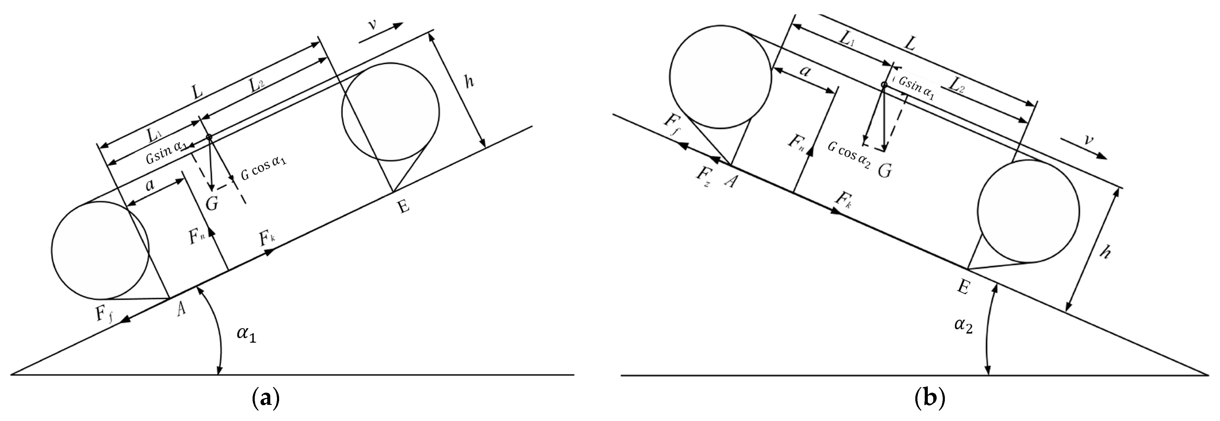
2.3.1. Uphill Rearward Tilt Limit Angle Analysis

Before the stability analysis, it is necessary to analyze the position of the center of mass of the track, according to the SolidWorks software [17] tool. To analyze the position of the center of mass of the assembly, when fully loaded, the height of the center of mass from the ground $h=205 \mathrm{mm}$, the distance from the center of the front support wheel $L_1=554 \mathrm{mm}$, the distance from the center of the rear support wheel $L_2=446 \mathrm{mm}$, and the track gauge of the track chassis $B=800 \mathrm{mm}$.

When the slope is too steep, the prototype will tip and roll over, or slip due to insufficient adhesion, so it is necessary to analyze the prototype’s uphill rearward limit tipping angle ${\alpha }_1$, downhill forward limit tipping angle ${\alpha }_2$, and lateral limit side tilting angle $\delta$, as well as the slip stabilization angle $\varphi$.

Regarding the prototype climbing process, if the slope gradient is great enough, backward instability will occur. Assuming that the prototype driving uphill and downhill at a constant speed, the force analysis is shown in Figure 5.

If the prototype is destabilized by backward tilting, it is tilted from point A. Taking the moment at point A, the moment equilibrium equation can be obtained:

$${\mathrm{F}}_{\mathrm{n}}\cdot \mathrm{a}+\mathrm{Gh}\sin {\alpha }_1-G{L}_1\cos {\alpha }_1=0$$

(11)

$$\mathrm{a}=\frac{G{L}_1\cos {\alpha }_1-\mathrm{Gh}\sin {\alpha }_1}{{\mathrm{F}}_{\mathrm{n}}}$$

(12)

where $\mathrm{a}$ is the width of the non-pedestrian side.

If the slope angle ${\alpha }_1$ increases, the support force of the slope on the prototype will then move backward until it coincides with the rear support wheel grounding point A, at which time the prototype will be rearwardly tilted and destabilized. The uphill rear tilt limit angle is given by Equation (13):

$${\mathsf{\alpha }}_1\le {\tan }^{-1}\frac{{\mathrm{L}}_1}{\mathrm{h}}=69.68°$$

(13)

2.3.2. Downhill Forward Tilt Limit Angle Analysis

During the downhill movement process of the prototype, if the slope gradient is large enough, forward instability will occur. If the prototype experiences forward tilting instability, it tilts from point E. Taking the moment at point E, the moment equilibrium equation can be obtained:

$${\mathrm{F}}_{\mathrm{n}}\cdot \left(L-\mathrm{a}\right)+\mathit{Gh}\sin {\alpha }_2-G\left(L-{\mathrm{L}}_1\right)\cos {\alpha }_2=0$$

(14)

$$L-\mathrm{a}=\frac{G\left(L-{\mathrm{L}}_1\right)\cos {\alpha }_2-\mathit{Gh}\sin {\alpha }_2}{{\mathrm{F}}_{\mathrm{n}}}$$

(15)

The downhill rear tilt limit angle is given by Equation (16):

$${\alpha }_2\le {\tan }^{-1}\frac{{L-L}_1}{h}=65.31°$$

(16)

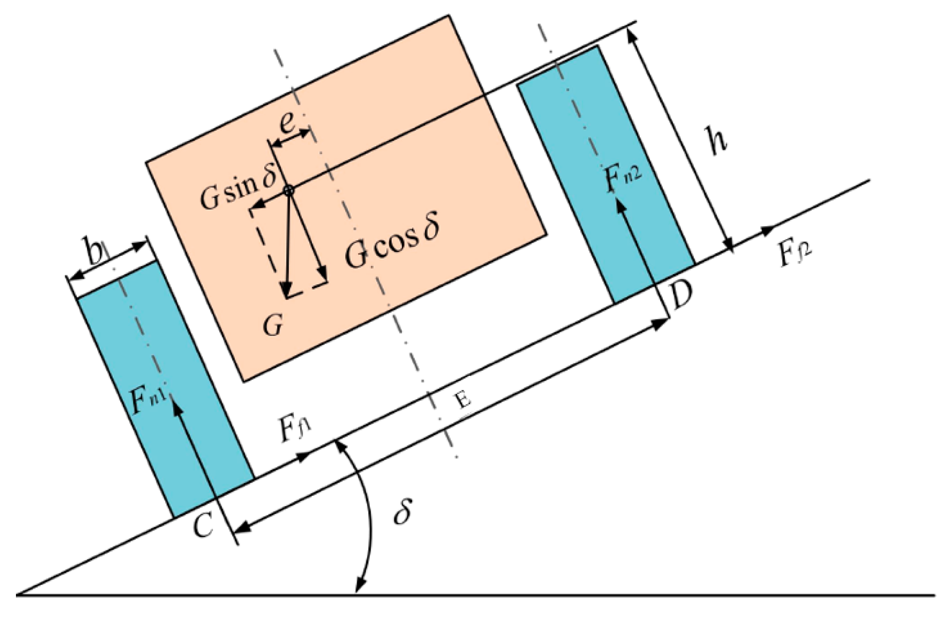
2.3.3. Cross-Slope Tilt Limit Angle Analysis

When the prototype is traveling on a cross-slope, if the slope gradient is large, dangerous conditions such as lateral tipping and lateral slip will occur. Assuming that the prototype is traveling on a cross-slope at a constant speed, its free-body diagram is shown in Figure 6.

According to the moment equilibrium, the moment is taken for point C, and the moment equilibrium equation can be obtained:

$${\mathrm{F}}_{\mathrm{n}2}B+\mathit{Gh}\mathit{sin}\delta -G\left(\frac{B}{2}-e\right)\mathit{cos}\delta =0$$

(17)

$${\mathrm{F}}_{\mathrm{n}2}=\frac{G\left(\frac{B}{2}-e\right)\mathit{cos}\delta -\mathit{Gh}\mathit{sin}\delta }{B}$$

(18)

where $e$ is the eccentricity of the center of mass with respect to the center plane of the track.

The limit angle of cross-slope tilt is given by Equation (19):

$$\delta \le {\tan }^{-1}\frac{0.5B-e}{h}=55.65°$$

(19)

2.3.4. Slip Stability Angle Analysis

Slip stability during travel on slopes is determined by the slip stability angle, which is usually determined by the attachment coefficient between the track and the ground, calculated as follows:

$$\varphi ={\tan }^{-1}\phi =41.98°$$

(20)

In summary, the prototype longitudinal and cross-slope driving tipping angle and slope driving slip stability angle are much larger than the designed maximum driving slope angle, and through the calibration, the prototype meets the design requirements and stability requirements.

2.4. Through Performance Analysis

Through performance analysis refers to the ability to pass over road obstacles—the better the ability to cross obstacles, the better the prototype’s ability to adapt to complex terrain. Its passing performance index is mainly the maximum height of the obstacle and the maximum width of the ditch.

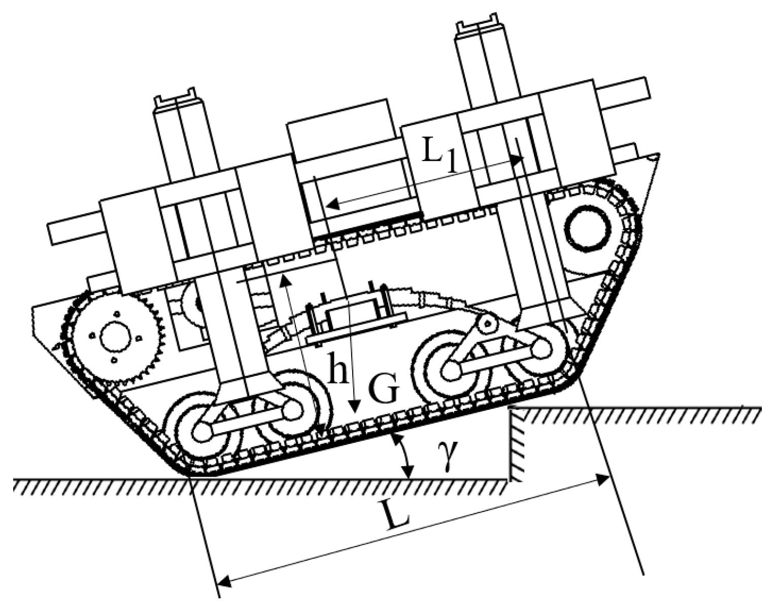
2.4.1. Obstacle Crossing Analysis

An important measure of the prototype’s barrier-passing ability is the maximum height of a vertical step that it can pass over. The center of mass position and the related track chassis design parameters will affect the prototype’s through performance. When the prototype passes over the step, the front end of the track comes into contact with the step, and the track keeps driving, driving the friction between the track teeth and the step, so that the prototype climbs forward, and the front section of the supporting wheels are lifted up, and when the center of mass reaches the maximum height, the prototype’s tail end is lifted up, and the center of mass is lowered, so that the vehicle passes over the step and travels forward, and the prototype passes over the step, as shown in the diagram in Figure 7, with the expression of the height of the prototype H being as follows:

$$H=\left(L-L_1-h\tan \gamma \right)\sin \gamma$$

(21)

where H is the vertical height of the step, and $\gamma$ is the tilt angle of the crawler conveyor.

The two important through performance indexes of the prototype are the approach angle and departure angle, and the larger the values of each, the better the through performance. The larger the approach angle, the larger the track grounding length, and the lower the grounding specific pressure, and at the same time, the number of teeth in contact between the track and the drive wheel decreases, resulting in greater stress on the drive wheel and increased wear on the drive wheel, meaning that the prototype should adopt the appropriate approach and departure angles. Factors affecting the prototype include the radius of the driving wheel, the center of gravity’s position, the track grounding length and the ground conditions. The longer the grounding length and the further forward the center of gravity position, the higher a vertical step that the prototype can pass over.

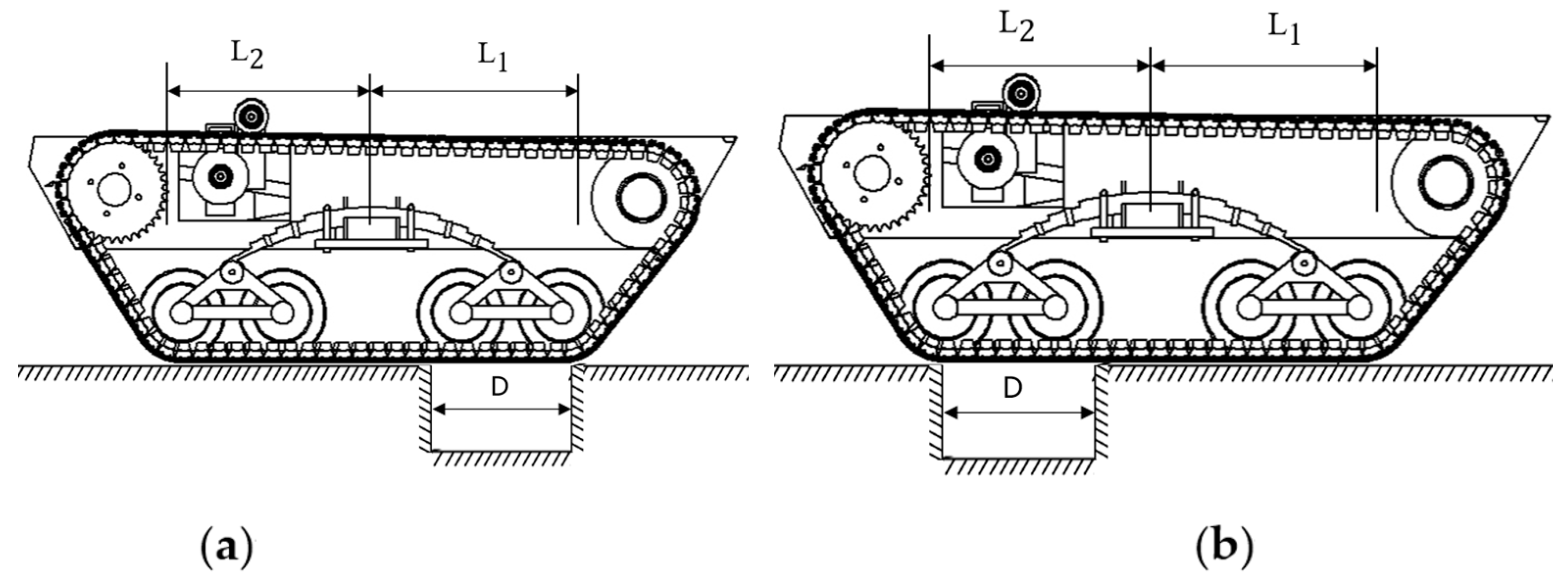
2.4.2. Over-Groove Analysis

The prototype over-groove performance is mainly determined by the gully width and the prototype over-groove width—the larger the width, the better its through performance, assuming that the prototype has a high stiffness to support the weight of the entire vehicle as well as a constant speed over the gully. The over-groove schematic is shown in Figure 8, where D is the gully width.

When the supporting wheel track comes into contact with the gully, if the center of mass of the prototype enters the gully, the supporting wheel will fall into the gully, and only when $L_1, L_2>B$ will the walking mechanism be able to cross the gully smoothly. Therefore, when designing the prototype, the center of mass should be located as close as possible to the center of the walking mechanism, so that the prototype can pass through as wide a gully as possible.

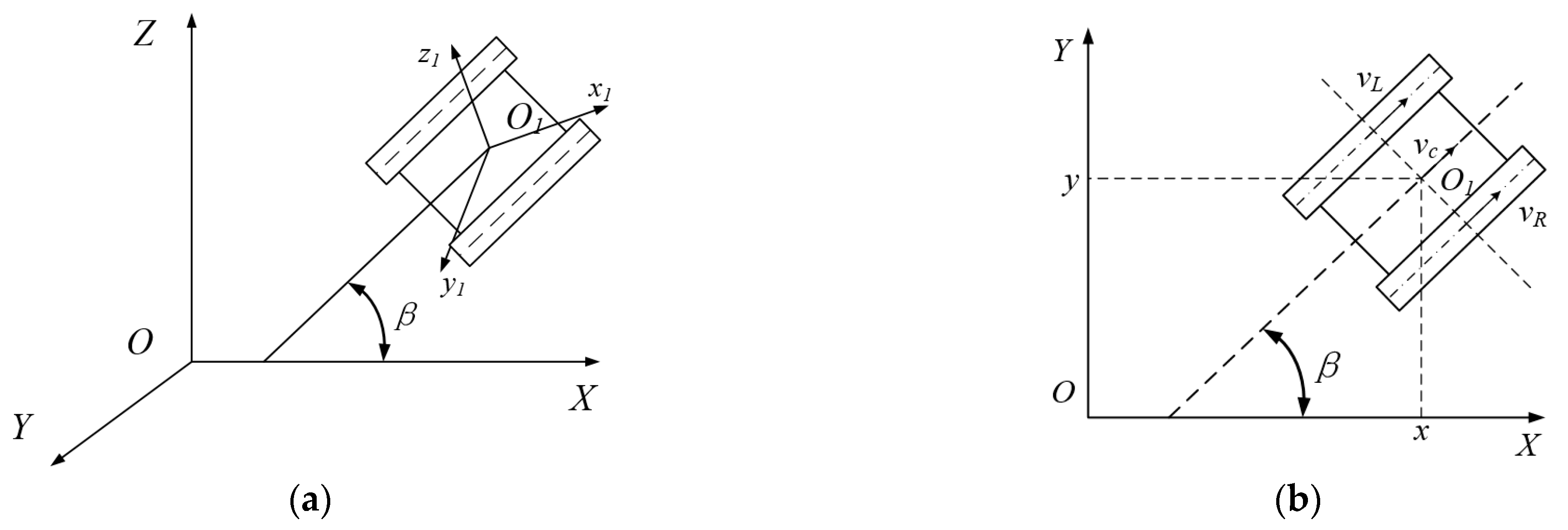
3. Kinematic Analysis

3.1. Establishment of Coordinate System

Because the tracks on both sides of the driving mechanism of the prototype are symmetrical to each other on the left and right sides, the center of symmetry $O_1$ is used as the coordinate system of the vehicle body when creating the kinematic coordinate system of the prototype, and the coordinate system of the vehicle body is a coordinate system that changes with the motion of the prototype, as shown in Figure 9a, with the geodetic coordinate system [18,19] of $O$. The kinematical equations of the prototype are established by using the RPY attitude descriptive method. The vehicle body rolls around the X-axis at a traverse angle of $\theta$, deflects around the Y-axis at a deflection angle of $\beta$, and pitches around the Z-axis at a pitch angle of $\omega$, and the prototype realizes steering around the Y-axis to travel when there is a speed difference between the left and right driving wheels.

The Euler angle is chosen to represent the change in spatial position of the prototype, and the prototype is set to rotate around the X-axis by $\theta$, around the Y-axis by $\omega$, and around the Z-axis by $\beta$. Therefore, the rotation matrix can be represented by the transformation matrix RPY $\left(\beta , \omega , \theta \right).$ It can be derived by the transformation:

$$\begin{array}{cc}\mathit{RPY}\left(\beta ,\omega ,\theta \right)\hfill & =\mathit{Rot}\left(z,\beta \right)\mathit{Rot}\left(y,\omega \right)\mathit{Rot}\left(x,\theta \right)\hfill \\ & =\left[\begin{array}{cccc}\cos \theta \cos \omega & \cos \theta \sin \omega \sin \beta -\sin \theta \cos \beta & \cos \theta \sin \omega \cos \beta +\sin \theta \sin \beta & 0\\ \sin \theta \cos \omega & \sin \theta \sin \omega \sin \beta +\cos \theta \cos \beta & \sin \theta \sin \omega \cos \beta -\cos \theta \sin \beta & 0\\ -\sin \omega & \cos \omega \sin \beta & \cos \omega \cos \beta & 0\\ 0& 0& 0& 1\end{array}\right]\end{array}$$

(22)

When the prototype’s plane movement in the body coordinate system, relative to the geodetic coordinate system, is equivalent to rotation around the Z-axis and an angle of $\beta$, it results in the prototype’s body coordinate system relative to the geodetic coordinate system of the transformation matrix, shown in Equation (23):

$$T=\left[\begin{array}{ccc}\cos \beta & -\sin \beta & 0\\ \sin \omega & \cos \omega & 0\\ 0& 0& 1\end{array}\right]$$

(23)

3.2. Kinematic Model of Prototype

The establishment of the coordinate system provides a spatial concept for the position of the prototype, and the next step is to model the kinematics of the prototype to represent the changes in displacement, angular velocity, etc., of the prototype at any given moment by establishing a mathematical model of the physical laws of motion. Before modeling the kinematics, the following assumptions are made:

(1)

The center of mass of the MSES virtual prototype is located at the center point of the vehicle, the driving surface is a hard surface, $O_1$ , and the shear force between the track and the ground is related to the shear displacement;

(2)

There is no relative sliding of the tracks against the drive wheels and no deformation of the tracks;

(3)

There is no lateral sliding of the prototype during steering;

(4)

When the prototype is steered, the coefficient of steering resistance is the same as the coefficient of resistance for straight-line driving;

(5)

The ground pressure of the prototype to the ground is linearly distributed.

Based on the above assumptions, the motion of the prototype in space is decomposed into the motion on the planar coordinate system XOY, as shown in Figure 9b, where $v_L$ and $v_R$ are the linear velocities of the left and right tracks, respectively, which are positive when they are in the same direction as the prototype’s center-of-mass velocity $v_c$ and negative when they are in the opposite direction, and $\beta$ is the angle of $v_c$ with the positive direction of the X-axis of the coordinate system.

$$\left\{\begin{array}{c}x=\frac{v_R+v_L}{2}\cdot v_c\cdot \cos \beta \\ y=\frac{v_R+v_L}{2}\cdot v_c\sin \beta \\ \beta =\frac{v_R-v_L}{B}\end{array}\right.$$

(24)

It can be seen that the prototype realizes its traveling path by controlling the speeds of the left and right tracks. When $v_R=v_L$, the prototype travels in a straight line; when $v_R>v_L$, the prototype travels to the right; when $v_R<v_L$, the prototype travels to the left; and when $v_R=-v_L$, the prototype performs a turn in the same place.

Integrating Equation (24), the coordinates of the center of mass position during planar motion of the prototype are obtained:

$$\left\{\begin{array}{c}x=\underset{0}{\overset{t}{\int }}\dot{x}dt=\frac{1}{2}\underset{0}{\overset{t}{\int }}\left(v_R+v_L\right)v_c\cdot \cos \beta \left(t\right)dt\\ y=\underset{0}{\overset{t}{\int }}\dot{y}dt=\frac{1}{2}\underset{0}{\overset{t}{\int }}\left(v_R+v_L\right)v_c\cdot \sin \beta \left(t\right)dt\\ \beta =\underset{0}{\overset{t}{\int }}\dot{\beta }dt=\frac{1}{B}\underset{0}{\overset{t}{\int }}\left(v_R-v_L\right)dt\end{array}\right.$$

(25)

4. Dynamics Analysis

4.1. Introduction to the Lagrange Equations

The Lagrange equations of the second class are a fundamental equation for solving dynamical problems, and the main process of establishing this dynamical equation [20] involves determining the degrees of freedom of the system and selecting the generalized coordinates; calculating the kinetic energy of the system by means of the generalized coordinates and the generalized velocities; computing the generalized force corresponding to the nonpotential forces; and substituting each of the above quantities into the Lagrange dynamical equations; and the Lagrange dynamical equations of the system can be obtained as follows:

$$\frac{d}{dt}\left(\frac{\partial T}{\partial \dot{q_{\mathrm{i}}}}\right)-\left(\frac{\partial T}{\partial q_i}\right)=Q_i i=1,2,\dots ,n$$

(26)

where $T$ is the kinetic energy of the system; $q_i$ is the generalized coordinate; $Q_i$ is the generalized force; and $n$ is the number of generalized coordinates, which is the same as the degrees of freedom of the system.

If the potential energy of the system is separated from the equation (i.e., the potential energy $U\left(q_i\right)$ is introduced at the same time as the virtual work of the damping force $D\left(q_i\right)$, i.e., the effect of the viscous drag force on the system, which is proportional to the magnitude of the velocity and opposite to the velocity) is considered, the Lagrange kinetic equations can be expressed by Equation (27):

$$\frac{d}{dt}\left(\frac{\partial T}{\partial \dot{q_i}}\right)-\frac{\partial T}{\partial q_i}+\frac{\partial D}{\partial \dot{q_i}}+\frac{\partial U}{\partial q_i}=F_i$$

(27)

where $D$ is the potential energy function of the system; $U$ is the dissipation function of the system; and $F_i$ is the generalized force corresponding to $q_i$.

4.2. Dynamics Modeling

The prototype machine works in a harsh environment underground, the working conditions are complex, and the structure of the prototype machine model is also relatively complex. In order to facilitate problem solving, the longitudinal model of the walking mechanism is simplified, and the prototype machine adopts rubber tracks, which is inconvenient for carrying out dynamics analysis, so the tracks are viewed as a section of the track plate connected together, and in accordance with the dynamics modeling theory and method, the discrete body dynamics modeling method is adopted, and the tracks are concentrated into a mass block. Other structures of the travel system are simplified in the longitudinal plane such as the drive wheel, guide wheel, support wheel, track frame, half shaft, driven gear, active gear, drive shaft and motor, etc. The following assumptions are made to simplify the dynamic model of the prototype travel system for easy analysis:

(1)

The MSES virtual prototype driving system passes through the same ground conditions on both sides of the tracks;

(2)

There is longitudinal symmetry of the prototype driving system, body, etc., to the center of mass;

(3)

The parts of the driving system of the prototype ignore their elastic variations, and the mass of each part is concentrated at the center of each part;

(4)

The driving system dynamics is described by a rigid system with spring stiffness and damping stiffness at the joints of the parts;

(5)

The track plates are of the same specification, with the same elastic properties, linear properties, stiffness coefficients and damping coefficients, and the ground attachment coefficient and sliding friction coefficient to the tracks are unchanged.

Based on the above analysis, the longitudinal 14-degree-of-freedom dynamics model of the prototype driving system was established, as shown in Figure 10.

In this figure, I, II, III and IV represent the driving wheel, guide wheel, front supporting wheel and rear supporting wheel, respectively. $M$ is the driving moment. $m_1, m_2, m_3, \mathrm{and} m_4$ are the centralized mass of the lower supporting track of the crawler travel system, respectively. $x_1, x_2, x_3, \mathrm{and} x_4$ are the longitudinal vibration displacement of the lower supporting track of the crawler travel system, respectively. $k_1, k_2, k_3, \mathrm{and} k_4$ are the stiffness coefficients of the lower support track of the crawler travel system, respectively. $c_1, c_2, c_3, {\mathrm{and} c}_4$ are the damping coefficients of the lower support track of the crawler travel system, respectively. $m_5$ is the centralized mass of the upper support track of the crawler travel system. $x_5$ is the longitudinal vibration displacement of the upper support track of the crawler travel system. $k_5 \mathrm{and} k_6$ are the stiffness coefficient. $c_5 \mathrm{and} c_6$ are the damping coefficients of the upper support track of the crawler travel system. $m_6, m_7, m_8, m_9, {\mathrm{and} m}_{10}$ are the masses of the half-shaft, driven gear, active gear, drive shaft and crawler frame, respectively. $x_6, x_7, x_8, x_9, \mathrm{and} x_{10}$ are the longitudinal vibration displacement of the half-shaft, driven gear, active gear, drive shaft and crawler frame, respectively. ${\theta }_1, {\theta }_2, {\theta }_3, \mathrm{and} {\theta }_4$ are the turning angles of the driving wheel, guide wheel, front support wheel and rear support wheel, respectively. $k_e \mathrm{and} c_e$ are the meshing stiffness and damping coefficient between the driving wheel and the track, respectively. $k_7 \mathrm{and} { c}_7$ are the stiffness coefficient and damping coefficient between the driving wheel and the half-shaft, respectively. $k_8 \mathrm{and} c_8$ are the stiffness coefficient and damping coefficient between the half-shaft and the driven gear, respectively. $k_9 \mathrm{and} c_9$ are the stiffness coefficient and damping coefficient between the driven gear and the active gear, respectively. $k_{10} \mathrm{and} c_{10}$ are the stiffness coefficient and damping coefficient between the main gear and the drive shaft, respectively. $k_{11},c_{11}, k_{12}, \mathrm{and} c_{12}$ are the stiffness coefficient and damping coefficient between the track frame and the driving and guiding wheels, respectively. $k_{13},c_{13}, k_{14}, \mathrm{and} c_{14}$ are the stiffness coefficient and damping coefficient between the track block and the front and rear supporting wheels, respectively. $k_{15},c_{15}, k_{16}, \mathrm{and} c_{16}$ are the stiffness coefficient and damping coefficient between the track frame and the front and rear supporting wheels, respectively.

4.3. Dynamics Modeling

Based on the dynamics model established in Section 4.2, the longitudinal dynamics equations of the tracked walking system are established:

$$\begin{array}{c}T=\frac{1}{2}{m}_1\dot{x_1^2}+\frac{1}{2}{m}_2\dot{x_2^2}+\frac{1}{2}{m}_3\dot{x_3^2}+\frac{1}{2}{m}_4\dot{x_4^2}+\frac{1}{2}{m}_5\dot{x_5^2}+\frac{1}{2}{m}_6\dot{x_6^2}+\frac{1}{2}{m}_7\dot{x_7^2}\\ +\frac{1}{2}{m}_8\dot{x_8^2}+\frac{1}{2}{m}_9\dot{x_9^2}+\frac{1}{2}{m}_{10}\dot{x_{10}^2}+\frac{1}{2}{J}_1\dot{{\theta }_1^2}+\frac{1}{2}{J}_2\dot{{\theta }_2^2}+\frac{1}{2}{J}_3\dot{{\theta }_3^2}+\frac{1}{2}{J}_4\dot{{\theta }_4^2}\end{array}$$

(28)

where $J_1,J_2, J_3, {\mathrm{and} J}_4$ are the moment of inertia of the driving wheel, guiding wheel, front supporting wheel and rear supporting wheel, respectively. $\dot{{\theta }_1},\dot{{\theta }_2}, \dot{{\theta }_3}, \mathrm{and} \dot{{\theta }_4}$ are the rotational speeds of the driving wheel, guiding wheel, front supporting wheel and rear supporting wheel, respectively.

$$\begin{array}{c}\mathrm{U}=\frac{1}{2}{K}_e{\left(R_1{\theta }_1-x_1\right)}^2+\frac{1}{2}{K}_1{\left(x_1-x_2\right)}^2+\frac{1}{2}{K}_2{\left(x_2-x_3\right)}^2+\frac{1}{2}{K}_3{\left(x_3-x_4\right)}^2\hfill \\ +\frac{1}{2}{K}_4{\left(x_4-R_2{\theta }_2\right)}^2+\frac{1}{2}{K}_5{\left(R_2{\theta }_2-x_5\right)}^2+\frac{1}{2}{K}_6{\left(x_5-R_1{\theta }_1\right)}^2\hfill \\ +\frac{1}{2}{K}_7{\left(x_6-R_1{\theta }_1\right)}^2+\frac{1}{2}{K}_8{\left(x_7-x_6\right)}^2+\frac{1}{2}{K}_9{\left(x_8-x_7\right)}^2\hfill \\ +\frac{1}{2}{K}_{10}{\left(x_9-x_8\right)}^2+\frac{1}{2}{K}_{11}{\left(x_{10}-R_1{\theta }_1\right)}^2+\frac{1}{2}{K}_{12}{\left(R_2{\theta }_2-x_{10}\right)}^2\hfill \\ +\frac{1}{2}{K}_{13}{\left(R_3{\theta }_4-x_2\right)}^2+\frac{1}{2}{K}_{14}{\left(R_3{\theta }_3-x_3\right)}^2\hfill \\ +\frac{1}{2}{K}_{15}{\left(x_{10}-R_3{\theta }_4\right)}^2+\frac{1}{2}{K}_{16}{\left(x_{10}-R_3{\theta }_3\right)}^2-\sum _{i=1}^8\delta m_i{gx}_i\sin \alpha \hfill \\ +\frac{2J_1}{R_1}g{\theta }_1\sin \alpha +\frac{2J_2}{R_2}g{\theta }_2\sin \alpha +\frac{2J_3}{R_3}g{\theta }_3\sin \alpha +\frac{2J_4}{R_4}g{\theta }_4\sin \alpha \hfill \end{array}$$

(29)

where $R_1, R_2, R_3$ are the radius of the driving wheel, guide wheel and supporting wheel, respectively. $\delta =\left\{\begin{array}{c}1,\theta >0\\ 0,\theta =0\\ 1,\theta <0\end{array}\right.$.

$$\begin{array}{c}\mathrm{D}=\frac{1}{2}{c}_e{\left(R_1{\theta }_1-\dot{x_1}\right)}^2+\frac{1}{2}{c}_1{\left(\dot{x_1}-\dot{x_2}\right)}^2+\frac{1}{2}{c}_2{\left(\dot{x_2}-\dot{x_3}\right)}^2+\frac{1}{2}{c}_3{\left(\dot{x_3}-\dot{x_4}\right)}^2\\ +\frac{1}{2}{c}_4{\left(\dot{x_4}-R_2\dot{{\theta }_2}\right)}^2+\frac{1}{2}{c}_5{\left(R_2{\dot{\theta }}_2-\dot{x_5}\right)}^2+\frac{1}{2}{c}_6{\left(\dot{x_5}-R_1\dot{{\theta }_1}\right)}^2\hfill \\ +\frac{1}{2}{c}_7{\left(\dot{x_6}-R_1\dot{{\theta }_1}\right)}^2+\frac{1}{2}{c}_8{\left(\dot{x_7}-\dot{x_6}\right)}^2+\frac{1}{2}{c}_9{\left(\dot{x_8}-\dot{x_7}\right)}^2\hfill \\ +\frac{1}{2}{c}_{10}{\left(\dot{x_9}-\dot{x_8}\right)}^2+\frac{1}{2}{c}_{11}{\left(\dot{x_{10}}-R_1\dot{{\theta }_1}\right)}^2+\frac{1}{2}{c}_{12}{\left(R_2{\dot{\theta }}_2-\dot{x_{10}}\right)}^2\hfill \\ +\frac{1}{2}{c}_{13}{\left(R_3\dot{{\theta }_4}-\dot{x_2}\right)}^2+\frac{1}{2}{c}_{14}{\left(R_3\dot{{\theta }_3}-\dot{x_3}\right)}^2+\frac{1}{2}{c}_{15}{\left(\dot{x_{10}}-R_3\dot{{\theta }_4}\right)}^2\hfill \\ +\frac{1}{2}{c}_{16}{\left(\dot{x_{10}}-R_3\dot{{\theta }_3}\right)}^2+\frac{1}{2}c\dot{x_2^2}+\frac{1}{2}c\dot{x_3^2}\hfill \end{array}$$

(30)

Substituting the above equation into the Lagrange equation yields the following equation:

$$m_1\ddot{x_1}-c_e{R}_1\dot{{\theta }_1}+c_e\dot{x_1}+c_1\dot{x_1}-c_1\dot{x_2}-k_e{R}_1{\theta }_1+k_e{x}_1+k_1{x}_1-k_1{x}_2=\delta m_{1}g\sin \alpha$$

(31)

$$\begin{array}{c}{m}_2\ddot{x_2}-c_1\dot{x_1}+c_1\dot{x_2}+c_2\dot{x_2}-c_1\dot{x_3}-c_{13}{R}_3\dot{{\theta }_4}+c_{13}\dot{x_2}-k_1{x}_1+k_1{x}_2+k_2{x}_2\\ -k_2{x}_3-k_{13}{R}_3{\theta }_4+k_{13}{x}_2=\delta m_{2}g\sin \alpha \end{array}$$

(32)

$$\begin{array}{c}{m}_3\ddot{x_3}-c_2\dot{x_2}+c_2\dot{x_3}+c_3\dot{x_3}-c_3\dot{x_4}-c_{14}{R}_3\dot{{\theta }_3}+c_{14}\dot{x_3}-k_{14}\dot{x_3}+c\dot{x_3}-k_2{x}_2+k_2{x}_3+k_3{x}_3\\ -k_3{x}_4-{k_{14}R}_3{\theta }_4+k_{14}{x}_3=\delta m_{3}g\sin \alpha \end{array}$$

(33)

$$m_4\ddot{x_4}-c_3\dot{x_3}+c_3\dot{x_4}-c_4{R}_2\dot{{\theta }_2}-k_3{x}_3+k_3{x}_4+k_4{x}_4-{k_{4}R}_2{\theta }_2=\delta m_{4}g\sin \alpha$$

(34)

$$m_5\ddot{x_5}-c_5{R}_2\dot{{\theta }_2}+c_5\dot{x_5}+c_6\dot{x_5}-c_6{R}_1\dot{{\theta }_1}-{k_{5}R}_2{\theta }_2+k_5{x}_5+k_6{x}_5-{k_{6}R}_1{\theta }_1=\delta m_{5}g\sin \alpha$$

(35)

$$m_6\ddot{x_6}+c_7\dot{x_6}-c_7{R}_1\dot{{\theta }_1}-c_8\dot{x_7}+c_8\dot{x_6}+k_7{x}_6-{k_{7}R}_1{\theta }_1-k_8{x}_7+k_8{x}_6=\delta m_{6}g\sin \alpha$$

(36)

$$m_7\ddot{x_7}+c_8\dot{x_7}-c_8\dot{x_6}-c_9\dot{x_8}+c_9\dot{x_7}+k_8{x}_7-k_8{x}_6-k_9{x}_8+k_9{x}_7=\delta m_{7}g\sin \alpha$$

(37)

$$m_8\ddot{x_8}+c_9\dot{x_8}-c_9\dot{x_7}-c_{10}\dot{x_9}+c_{10}\dot{x_8}+k_9{x}_8-k_9{x}_7-k_{10}{x}_9+k_{10}{x}_8=\delta m_{8}g\sin \alpha$$

(38)

$$m_9\ddot{x_9}+c_{10}\dot{x_9}-c_{10}\dot{x_8}+k_{10}{x}_9-k_{10}{x}_8=\delta m_{9}g\sin \alpha$$

(39)

$$\begin{gathered} m_{10}{\ddot{x}}_{10}+c_{11}{\dot{x}}_{10}-c_{11}{R}_1{\dot{\theta }}_1-c_{12}{R}_2{\dot{\theta }}_2+c_{12}{\dot{x}}_{10}+c_{15}{\dot{x}}_{10}-c_{15}{R}_3{\dot{\theta }}_4+c_{16}{\dot{x}}_{10}-c_{16}{R}_3{\dot{\theta }}_3+k_{11}{x}_{10}-k_{11}{R}_1{\theta }_1 \\ -k_{12}{R}_2{\theta }_2+k_{12}{x}_{10}+k_{15}{x}_{10}-k_{15}{R}_3{\theta }_4+k_{16}{x}_{10}-k_{16}{R}_3{\theta }_3=\delta m_{10}\mathrm{g}\sin \mathsf{\alpha } \end{gathered}$$

(40)

$$\begin{gathered} J_1{\ddot{\theta }}_1+c_e{R}_1^2{\dot{\theta }}_1-c_e{R}_1{\dot{x}}_1-c_6{R}_1{\dot{x}}_5+c_6{R}_1^2{\dot{\theta }}_1-c_7{R}_1{\dot{x}}_6+c_7{R}_1^2{\dot{\theta }}_1-c_{11}{R}_1{\dot{x}}_{10}+c_{11}{R}_1^2{\dot{\theta }}_1+k_e{R}_1^2{\theta }_1-k_e{R}_1{x}_1 \\ -k_6{R}_1{x}_5+k_6{R}_1^2{\theta }_1-k_7{R}_1{x}_6+k_7{R}_1^2{\theta }_1-k_{11}{R}_1{x}_{10}+k_{11}{R}_1^2{\theta }_1=M-\mathsf{\delta }\frac{2J_1}{R_1}\mathrm{g}\sin \mathsf{\alpha } \end{gathered}$$

(41)

$$\begin{gathered} J_2{\ddot{\theta }}_2-c_4{R}_2{\dot{x}}_4+c_4{R}_2^2{\dot{\theta }}_2+c_5{R}_2^2{\dot{\theta }}_2-c_5{R}_2{\dot{x}}_5+c_{12}{R}_2^2{\dot{\theta }}_2-c_{12}{R}_2{\dot{x}}_{10}-k_4{R}_2{x}_4+k_4{R}_2^2{\theta }_2+k_5{R}_2^2{\theta }_2-k_5{R}_2{x}_5 \\ +k_{12}{R}_2^2{\theta }_2-k_{12}{R}_2{x}_{10}=-\mathsf{\delta }\frac{2J_2}{R_2}\mathrm{g}\sin \mathsf{\alpha } \end{gathered}$$

(42)

$$J_3{\ddot{\theta }}_3+c_{14}{R}_3^2{\dot{\theta }}_3-c_{14}{R}_3{\dot{x}}_3-c_{16}{R}_3{\dot{x}}_{10}+c_{16}{R}_3^2{\dot{\mathsf{\theta }}}_3+k_{14}{R}_3^2{\mathsf{\theta }}_3-k_{14}{R}_3{x}_3-k_{16}{R}_3{x}_{10}+k_{16}{R}_3^2{\mathsf{\theta }}_3=-\mathsf{\delta }\frac{2J_3}{R_3}\mathrm{g}\sin \mathsf{\alpha }$$

(43)

$$J_4{\ddot{\mathsf{\theta }}}_4+c_{13}{R}_3^2{\dot{\mathsf{\theta }}}_4-c_{13}{R}_3{\dot{x}}_2-c_{15}{R}_3{\dot{x}}_{10}+c_{15}{R}_3^2{\dot{\mathsf{\theta }}}_4+k_{13}{R}_3^2{\mathsf{\theta }}_4-k_{13}{R}_3{x}_2-k_{15}{R}_3{x}_{10}+k_{15}{R}_3^2{\mathsf{\theta }}_4=-\mathsf{\delta }\frac{2J_4}{R_3}\mathrm{g}\sin \mathsf{\alpha }$$

(44)

After finishing, the motion differential equation of the prototype driving system can be obtained:

$$M\ddot{X}+C\dot{X}+KX=F$$

(45)

where the matrix M is:

$$M=\left[\begin{array}{cccccccccccccc}{m}_1& 0& 0& 0& 0& 0& 0& 0& 0& 0& 0& 0& 0& 0\\ 0& m_2& 0& 0& 0& 0& 0& 0& 0& 0& 0& 0& 0& 0\\ 0& 0& m_3& 0& 0& 0& 0& 0& 0& 0& 0& 0& 0& 0\\ 0& 0& 0& m_4& 0& 0& 0& 0& 0& 0& 0& 0& 0& 0\\ 0& 0& 0& 0& m_5& 0& 0& 0& 0& 0& 0& 0& 0& 0\\ 0& 0& 0& 0& 0& m_6& 0& 0& 0& 0& 0& 0& 0& 0\\ 0& 0& 0& 0& 0& 0& m_7& 0& 0& 0& 0& 0& 0& 0\\ 0& 0& 0& 0& 0& 0& 0& m_8& 0& 0& 0& 0& 0& 0\\ 0& 0& 0& 0& 0& 0& 0& 0& m_9& 0& 0& 0& 0& 0\\ 0& 0& 0& 0& 0& 0& 0& 0& 0& m_{10}& 0& 0& 0& 0\\ 0& 0& 0& 0& 0& 0& 0& 0& 0& 0& J_1& 0& 0& 0\\ 0& 0& 0& 0& 0& 0& 0& 0& 0& 0& 0& J_2& 0& 0\\ 0& 0& 0& 0& 0& 0& 0& 0& 0& 0& 0& 0& J_3& 0\\ 0& 0& 0& 0& 0& 0& 0& 0& 0& 0& 0& 0& 0& J_4\end{array}\right]$$

(46)

The matrix C is:

$$C=\left[\begin{array}{cccccccccccccc}{C}_{\mathrm{1,1}}& {-c}_1& 0& 0& 0& 0& 0& 0& 0& 0& {-c}_e{R}_1& 0& 0& 0\\ {-c}_1& C_{\mathrm{2,2}}& {-c}_2& 0& 0& 0& 0& 0& 0& 0& 0& 0& 0& {-c}_{13}{R}_3\\ 0& {-c}_2& C_{\mathrm{3,3}}& {-c}_3& 0& 0& 0& 0& 0& 0& 0& 0& {-c}_{14}{R}_3& 0\\ 0& 0& {-c}_3& C_{\mathrm{4,4}}& 0& 0& 0& 0& 0& 0& 0& {-c}_4{R}_2& 0& 0\\ 0& 0& 0& 0& C_{\mathrm{5,5}}& 0& 0& 0& 0& 0& {-c}_6{R}_1& {-c}_5{R}_2& 0& 0\\ 0& 0& 0& 0& 0& C_{\mathrm{6,6}}& {-c}_8& 0& 0& 0& {-c}_7{R}_1& 0& 0& 0\\ 0& 0& 0& 0& 0& {-c}_8& C_{\mathrm{7,7}}& {-c}_9& 0& 0& 0& 0& 0& 0\\ 0& 0& 0& 0& 0& 0& {-c}_9& C_{\mathrm{8,8}}& {-c}_{10}& 0& 0& 0& 0& 0\\ 0& 0& 0& 0& 0& 0& 0& {-c}_{10}& C_{\mathrm{9,9}}& 0& 0& 0& 0& 0\\ 0& 0& 0& 0& 0& 0& 0& 0& 0& C_{\mathrm{10,10}}& {-c}_{11}{R}_1& {-c}_{12}{R}_2& {-c}_{16}{R}_3& {-c}_{15}{R}_3\\ {-c}_e{R}_1& 0& 0& 0& {-c}_6{R}_1& {-c}_7{R}_1& 0& 0& 0& {-c}_{11}{R}_1& C_{\mathrm{11,11}}& 0& 0& 0\\ 0& 0& 0& {-c}_4{R}_2& {-c}_5{R}_2& 0& 0& 0& 0& {-c}_{12}{R}_2& 0& C_{\mathrm{12,12}}& 0& 0\\ 0& 0& {-c}_{14}{R}_3& 0& 0& 0& 0& 0& 0& {-c}_{16}{R}_3& 0& 0& C_{\mathrm{13,13}}& 0\\ 0& {-c}_{13}{R}_3& 0& 0& 0& 0& 0& 0& 0& {-c}_{15}{R}_3& 0& 0& 0& C_{\mathrm{14,14}}\end{array}\right]$$

(47)

where $C_{\mathrm{1,1}}=c_e+c_1$; $C_{\mathrm{2,2}}=c_1+c_2+c_{13}+c$; $C_{\mathrm{3,3}}=c_2+c_3+c_{14}+c$; $C_{\mathrm{4,4}}=c_3+c_4$; $C_{\mathrm{5,5}}=c_5+c_6$; $C_{\mathrm{6,6}}=c_7+c_8$; $C_{\mathrm{7,7}}=c_8+c_9$; $C_{\mathrm{8,8}}=c_9+c_{10}$; $C_{\mathrm{9,9}}=c_{10}$; $C_{\mathrm{10,10}}=c_{11}+c_{12}+c_{15}+c_{16}$; $C_{\mathrm{11,11}}=\left(c_e+c_6+c_7+c_{11}\right)R_1^2$; $C_{\mathrm{12,12}}=\left(c_5+c_4+c_{12}\right)R_2^2$; $C_{\mathrm{13,13}}=\left(c_{14}+c_{16}\right)R_3^2$; and $C_{\mathrm{14,14}}=\left(c_{13}+c_{15}\right)R_3^2$.

The matrix K is:

$$K=\left[\begin{array}{cccccccccccccc}{K}_{\mathrm{1,1}}& {-k}_1& 0& 0& 0& 0& 0& 0& 0& 0& {-k}_e{R}_1& 0& 0& 0\\ {-k}_1& K_{\mathrm{2,2}}& {-k}_2& 0& 0& 0& 0& 0& 0& 0& 0& 0& 0& {-k}_{13}{R}_3\\ 0& {-k}_2& K_{\mathrm{3,3}}& {-k}_3& 0& 0& 0& 0& 0& 0& 0& 0& {-k}_{14}{R}_3& 0\\ 0& 0& {-k}_3& K_{\mathrm{4,4}}& 0& 0& 0& 0& 0& 0& 0& {-k}_4{R}_2& 0& 0\\ 0& 0& 0& 0& K_{\mathrm{5,5}}& 0& 0& 0& 0& 0& {-k}_6{R}_1& {-k}_5{R}_2& 0& 0\\ 0& 0& 0& 0& 0& K_{\mathrm{6,6}}& {-k}_8& 0& 0& 0& {-k}_7{R}_1& 0& 0& 0\\ 0& 0& 0& 0& 0& {-k}_8& K_{\mathrm{7,7}}& {-k}_9& 0& 0& 0& 0& 0& 0\\ 0& 0& 0& 0& 0& 0& {-k}_9& K_{\mathrm{8,8}}& {-k}_{10}& 0& 0& 0& 0& 0\\ 0& 0& 0& 0& 0& 0& 0& {-k}_{10}& K_{\mathrm{9,9}}& 0& 0& 0& 0& 0\\ 0& 0& 0& 0& 0& 0& 0& 0& 0& K_{\mathrm{10,10}}& {-k}_{11}{R}_1& {-k}_{12}{R}_2& {-k}_{16}{R}_3& {-k}_{15}{R}_3\\ {-k}_e{R}_1& 0& 0& 0& {-k}_6{R}_1& {-k}_7{R}_1& 0& 0& 0& {-k}_{11}{R}_1& K_{\mathrm{11,11}}& 0& 0& 0\\ 0& 0& 0& {-k}_4{R}_2& {-k}_5{R}_2& 0& 0& 0& 0& {-k}_{12}{R}_2& 0& K_{\mathrm{12,12}}& 0& 0\\ 0& 0& {-k}_{14}{R}_3& 0& 0& 0& 0& 0& 0& {-k}_{16}{R}_3& 0& 0& K_{\mathrm{13,13}}& 0\\ 0& {-k}_{13}{R}_3& 0& 0& 0& 0& 0& 0& 0& {-k}_{15}{R}_3& 0& 0& 0& K_{\mathrm{14,14}}\end{array}\right]$$

(48)

where $K_{\mathrm{1,1}}=k_e+k_1$; $K_{\mathrm{2,2}}=k_1+k_2+k_{13}$; $K_{\mathrm{3,3}}=k_2+k_3+k_{14}$; $K_{\mathrm{4,4}}=k_3+k_4$; $K_{\mathrm{5,5}}=k_5+k_6$; $K_{\mathrm{6,6}}=k_7+k_8$; $K_{\mathrm{7,7}}=k_8+k_9$; $K_{\mathrm{8,8}}=k_9+k_{10}$; $K_{\mathrm{9,9}}=k_{10}$; $K_{\mathrm{10,10}}=k_{11}+k_{12}+k_{15}+k_{16}$; $K_{\mathrm{11,11}}=\left(k_e+k_6+k_7+k_{11}\right)R_1^2$; $K_{\mathrm{12,12}}=\left(k_5+k_4+k_{12}\right)R_2^2$; $K_{13,13}=\left(k_{14}+k_{16}\right)R_3^2$; and $K_{14,14}=\left(k_{13}+k_{15}\right)R_3^2$.

The matrix X is:

$$\mathrm{X}={\left[\begin{array}{cccccccccccccc}{\mathrm{x}}_1& {\mathrm{x}}_2& {\mathrm{x}}_3& {\mathrm{x}}_4& {\mathrm{x}}_5& {\mathrm{x}}_6& {\mathrm{x}}_7& {\mathrm{x}}_8& {\mathrm{x}}_9& {\mathrm{x}}_{10}& {\mathsf{\theta }}_1& {\mathsf{\theta }}_2& {\mathsf{\theta }}_3& {\mathsf{\theta }}_4\end{array}\right]}^{\mathrm{T}}$$

(49)

The matrix F is:

$$\mathrm{F}=\left[\begin{array}{c}\mathsf{\delta }{\mathrm{m}}_1\mathrm{g}\sin \mathsf{\alpha }\\ \mathsf{\delta }{\mathrm{m}}_2\mathrm{g}\sin \mathsf{\alpha }\\ \mathsf{\delta }{\mathrm{m}}_3\mathrm{g}\sin \mathsf{\alpha }\\ \mathsf{\delta }{\mathrm{m}}_4\mathrm{g}\sin \mathsf{\alpha }\\ \mathsf{\delta }{\mathrm{m}}_5\mathrm{g}\sin \mathsf{\alpha }\\ \mathsf{\delta }{\mathrm{m}}_6\mathrm{g}\sin \mathsf{\alpha }\\ \mathsf{\delta }{\mathrm{m}}_7\mathrm{g}\sin \mathsf{\alpha }\\ \mathsf{\delta }{\mathrm{m}}_8\mathrm{g}\sin \mathsf{\alpha }\\ \mathsf{\delta }{\mathrm{m}}_9\mathrm{g}\sin \mathsf{\alpha }\\ \mathsf{\delta }{\mathrm{m}}_{10}\mathrm{g}\sin \mathsf{\alpha }\\ \mathrm{M}-\mathsf{\delta }\frac{{2\mathrm{J}}_1}{{\mathrm{R}}_1}\mathrm{g}\sin \mathsf{\alpha }\\ -\mathsf{\delta }\frac{{2\mathrm{J}}_2}{{\mathrm{R}}_2}\mathrm{g}\sin \mathsf{\alpha }\\ -\mathsf{\delta }\frac{{2\mathrm{J}}_3}{{\mathrm{R}}_3}\mathrm{g}\sin \mathsf{\alpha }\\ -\mathsf{\delta }\frac{{2\mathrm{J}}_4}{{\mathrm{R}}_3}\mathrm{g}\sin \mathsf{\alpha }\end{array}\right]$$

(50)

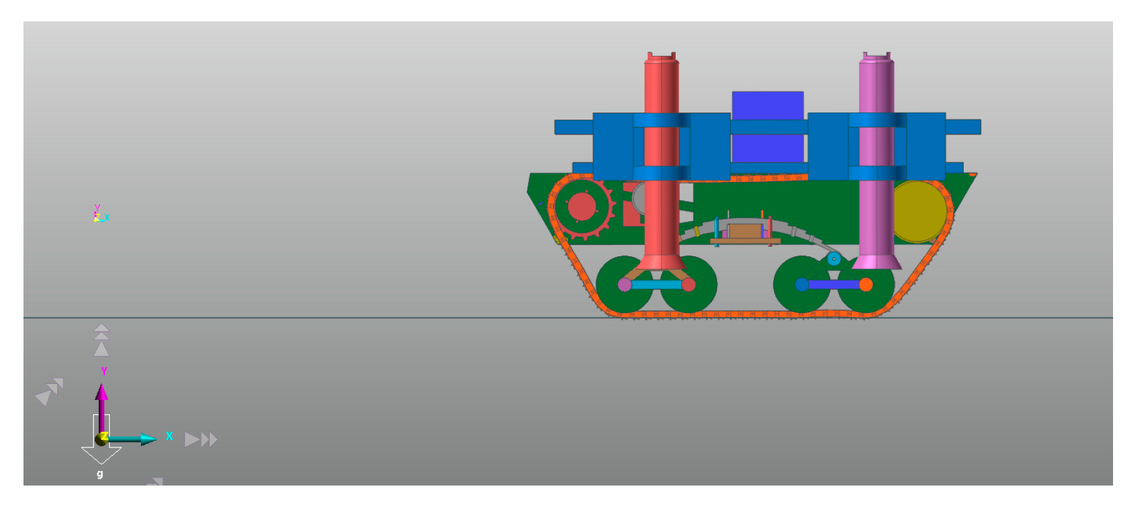
5. Multi-Body Dynamics Simulation

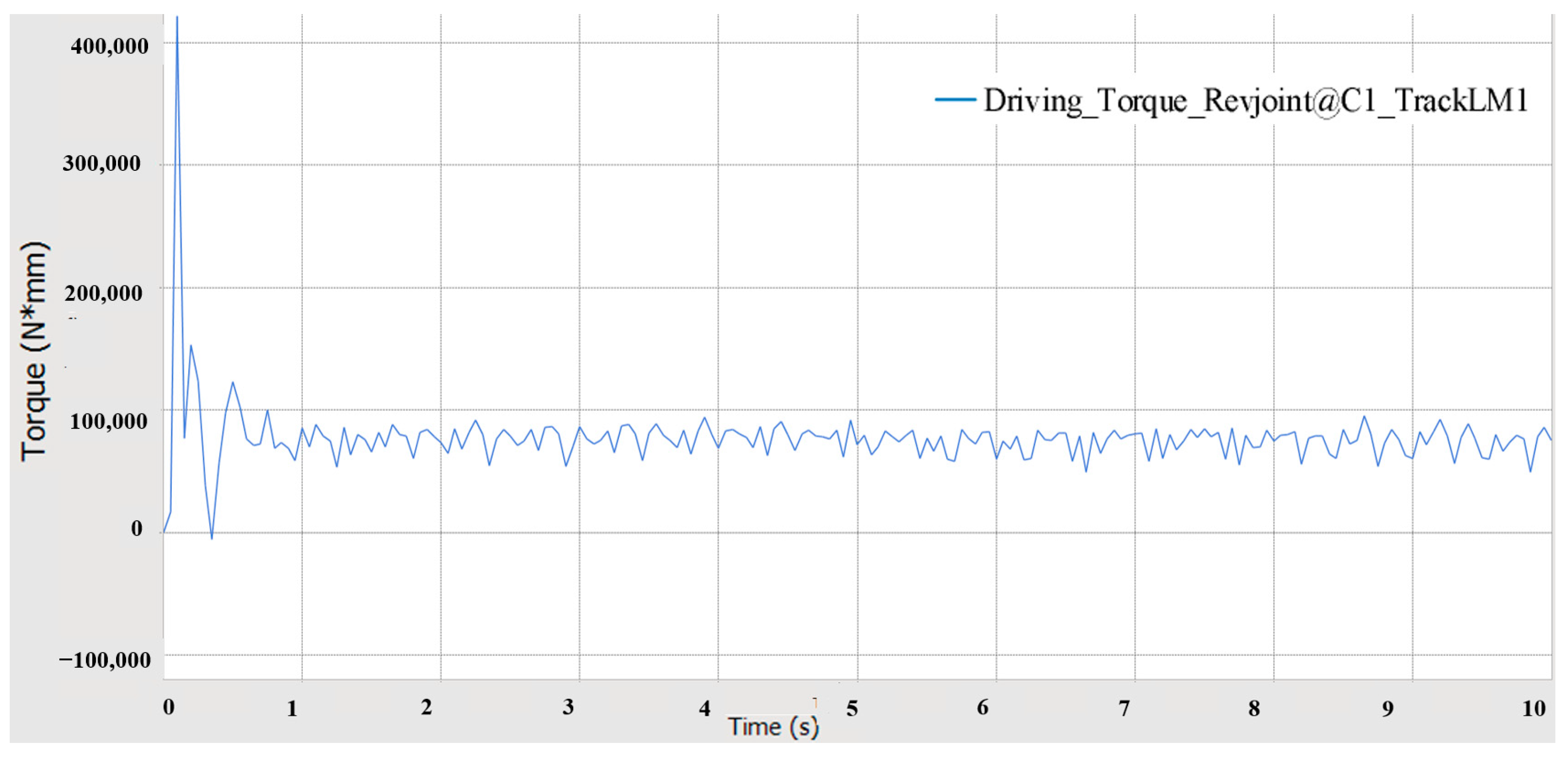
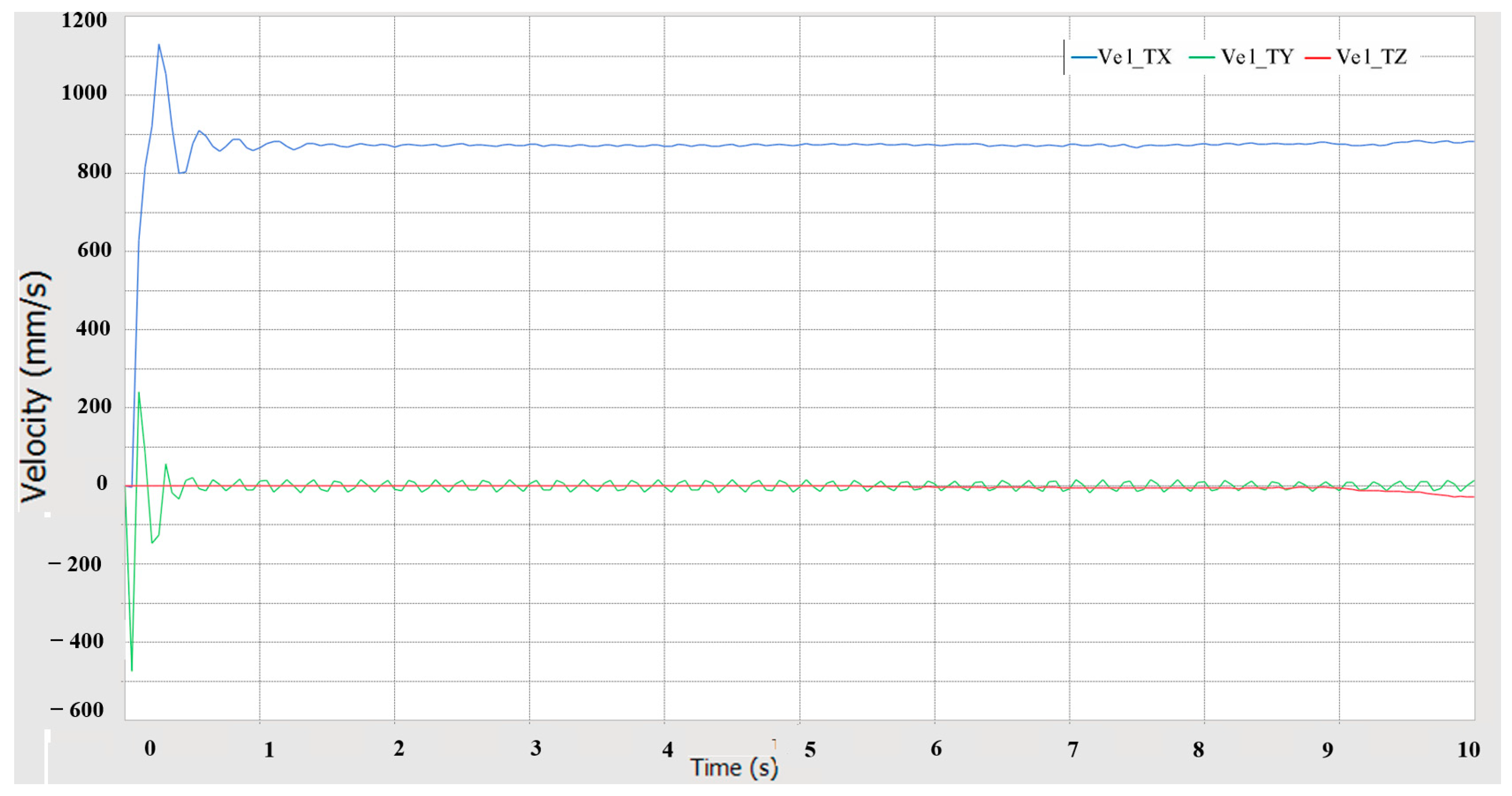
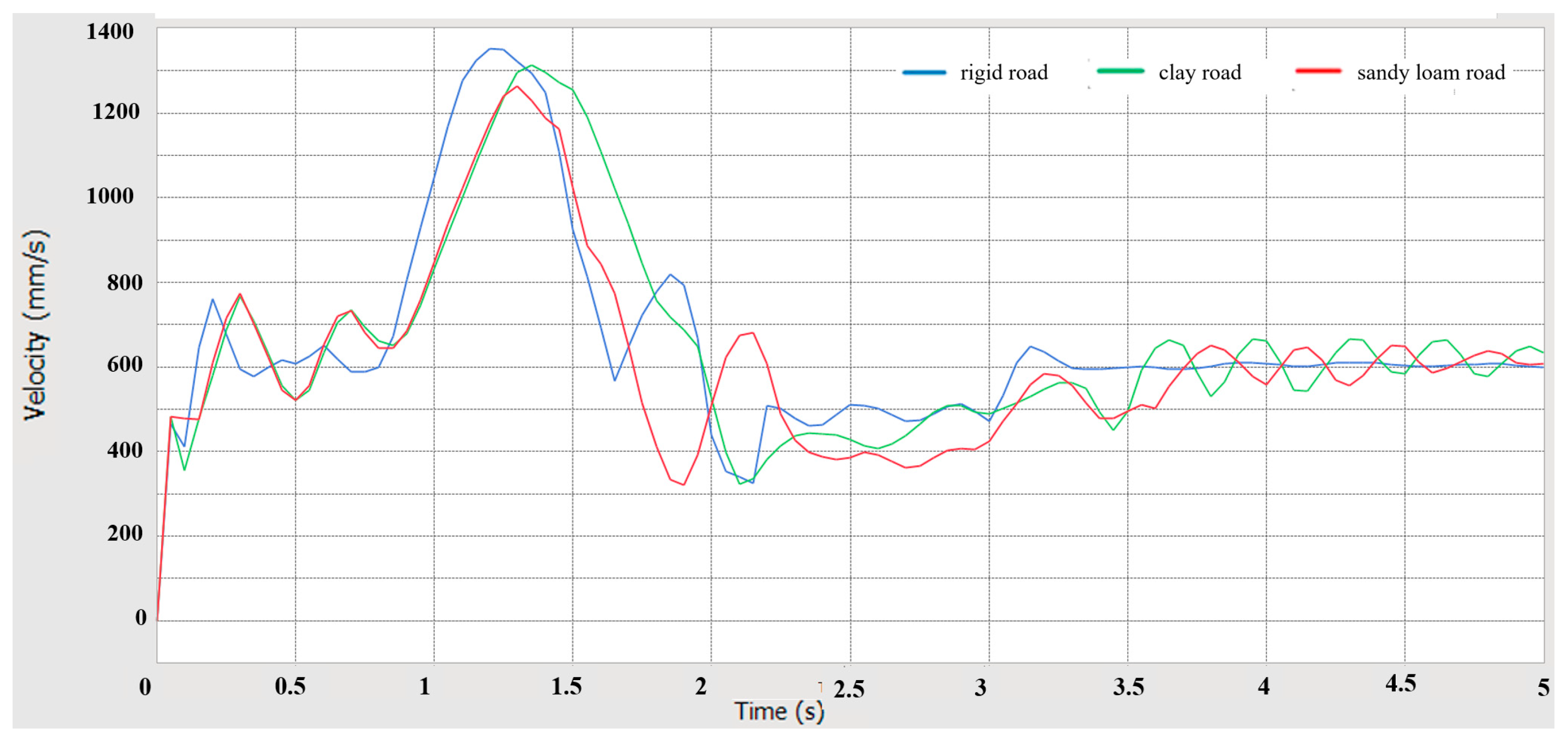
5.1. Driving Performance Simulation Analysis

The speed of the prototype is 3.6 km/h when traveling in a straight line on a flat road, the angular speed of the driving wheel is 10.1 rad/s, and the radius of the driving wheel is known to be 99 mm, from which the maximum driving torque $T_1$ and the maximum driving power $P_1$ of the prototype can be calculated:

$$T_1=\frac{1}{2}{F}_{1}r=126.13 \mathrm{N}\cdot \mathrm{m}$$

(51)

$${P_1=T}_1\omega =1.27 \mathrm{K}\mathrm{W}$$

(52)

The driving condition of the prototype on a flat road is shown in Figure 11, and the prototype is set to travel at 3.6 km/h in the positive direction along the X-axis, with a simulation time of 10 s and a step size of 200. The prototype advances in the positive direction along the X-axis, and the Y-axis is in the vertical direction, and the center of mass of the prototype is at the starting position of (24, 205, 1267).

The trend of the driving torque of the prototype is shown in Figure 12. In the first s, the prototype falls to the ground and accelerates, which leads to the oscillation of the prototype, and the torque changes are large; in the acceleration stage, the prototype is subjected to rolling resistance, internal resistance and inertial resistance at the same time, and the driving torque reaches a maximum of 122.85 $\mathrm{N}\cdot \mathrm{m}$, after which the prototype travels steadily, and the driving torque reaches a stable state.

From the figure, it can be seen that the drive torque variation is periodic, which is due to the effect of the presence of polygons in the drive of the track traveling system. The simulation results are shown in

Table 1. Comparison of straight driving simulation results.

	Simulation Value	Theoretical Value	Inaccuracy
Driving torque $\mathrm{N}\cdot \mathrm{m}$	122.85	126.13	2.6%
Driving power $\mathrm{K}\mathrm{W}$	1.24	1.27	2.6%

. This shows that the prototype tracked chassis and power system are reasonably designed and the prototype is highly reliable.

The speed change curve for each direction during the driving process of the prototype is shown in Figure 13. The speed fluctuates greatly in the first 0~0.3 s, which is caused by the collision between the prototype and the ground and acceleration at the beginning of the simulation, and when the prototype is running stably, the speed fluctuates narrowly up and down around 0.88 m/s due to the uneven force during the engagement process of the driving wheels and the track, the speeds of the Y and Z directions fluctuate narrowly up and down around zero. This kind of periodic fluctuation is unavoidable during the straight-line traveling of the prototype, which is consistent with the actual situation. It is verified that the prototype has strong stability and smoothness when traveling on a smooth road surface and meets the design requirements.

5.2. Anti-Rollover Performance Simulation Analysis

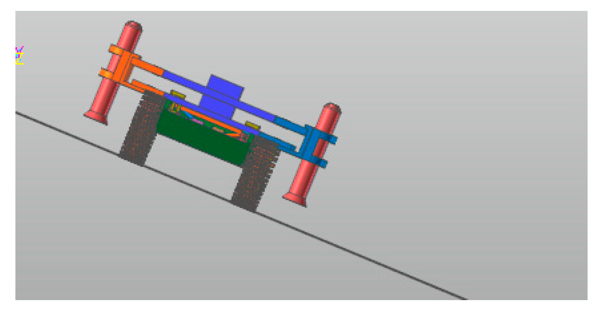
5.2.1. Uphill Driving Simulation Analysis

The climbing performance of the prototype is an important quality in order to overcome the sloping road type. We choose a driving speed of 2.5 km/h for climbing operation, meaning that the angular velocity of the driving wheel is 7 rad/s, from which the maximum driving torque of the prototype climbing $T_3$ and the maximum driving power $P_3$ can be calculated:

$${T_3=\frac{1}{2}F}_{3}r=298.05 \mathrm{N}\cdot \mathrm{m}$$

(53)

$${P_3=T}_3\omega =2.09 \mathrm{K}\mathrm{W}$$

(54)

Coal mine underground terrain is more complex, often demonstrating tunnel slope road conditions, and the slope is generally 15°, but usually not more than 25°. Coal mines mostly have sand and gravel road surfaces, but due to the unevenness of the ground, water may also exist on the road surface, making the road more complex. These factors will have an impact on the dynamic stability of the transport truck; therefore, the prototype’s performance in climbing with different gradients and different geologies under the dynamics of the simulation analysis is tested. Figure 14 shows the schematic diagram of the simulation process of the prototype on a 25° slope.

We establish a hard road model with slopes of 15°, 20° and 25°, set the speed of the prototype to 2.5 km/h, set the simulation time to 5 s, and set the step size to 100. The prototype first landed on a flat surface and accelerated, climbing at a constant speed, and finally entered the flat surface. This process is a complete slope climbing simulation process.

Figure 15 and Figure 16 show the curves of traveling speed and vibration acceleration of the prototype under different slopes, respectively. The simulation results show that the prototype does not overturn during the 25° slope driving, the speed and acceleration remain stable during the stable driving phase, the fluctuation amplitude is small during the transition phase, and it can return to the normal level quickly, which indicates that the prototype has strong dynamic stability and smoothness when driving on a slope, and it meets the design requirements.

We change the road surface parameters to establish a hard road surface, a clay road surface and a sandy loam road surface model to simulate the prototype’s ability to climb over a 25° ramp on different ground types. We set the prototype’s speed to 2.5 km/h, set the simulation time to 5 s and set the step size to 100. The simulation process is the same as the dynamics of the simulation of the different slopes. Figure 17 shows the speed change curve of the prototype under different ground surface conditions.

Figure 18 shows the change curve of the pitch angle of the prototype under different ground surface conditions. Pitch angle is one of the important indexes to measure the stability and through performance of slope climbing traveling—if the pitch angle is too large, it will cause dangerous conditions such as sliding or even tipping over. The simulation results show that the pitch angle of the prototype under different ground conditions is similar to the slope angle, and the change in the pitch angle is small, which indicates that the prototype has strong through performance and stability under different ground conditions of hill-climbing driving.

Figure 19 shows the variation curve of the driving torque of the prototype under different ground surfaces, from which it can be seen that the maximum torque is 287.69 $\mathrm{N}\cdot \mathrm{m}$ in the climbing stage. The climbing driving simulation results are shown in

Table 2. Comparison of climbing driving simulation results.

	Simulation Value	Theoretical Value	Inaccuracy
Driving torque $\mathrm{N}\cdot \mathrm{m}$	287.69	298.05	3.5%
Driving power $\mathrm{K}\mathrm{W}$	2.01	2.09	3.5%

.

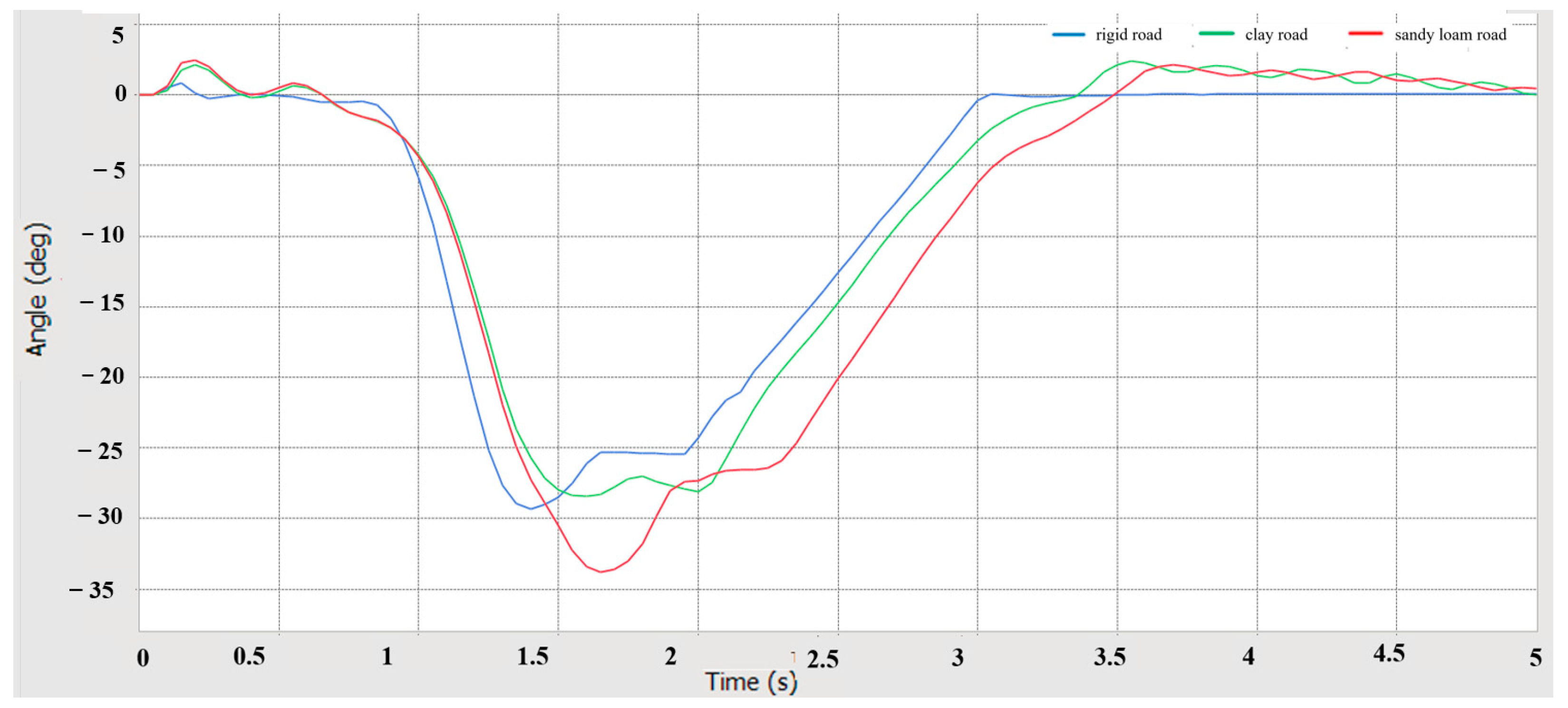
5.2.2. Downhill Driving Simulation Analysis

To study the downhill power stability of the prototype for different road conditions with a gradient of 25°, the speed setting is the same as that of the uphill driving condition, the simulation time is 5 s, and the step size is 100. In order to better verify the downhill driving stability of the prototype, the prototype is first accelerated on flat ground, then enters into the downhill driving stage, and finally enters into the flat ground driving stage during the simulation. Figure 20 shows the schematic diagram of the downhill driving condition of the prototype.

Figure 21 and Figure 22 show the speed and vibration acceleration curves of the prototype under different road conditions. From the simulation results, it can be seen that the speed and vibration acceleration of the prototype show small fluctuations during the transition phase from level ground to sloping ground; during the stable driving phase, the speed and acceleration remain stable, which indicates that the prototype has good dynamic stability.

Figure 23 shows the variation curve of the pitch angle of the prototype under different ground conditions. From the change curve, it can be seen that in the transition stage from flat ground to sloping ground, the pitch angle of the prototype produces a slight change, and in the downhill stable driving stage, it can be seen that the change in the pitch angle of the prototype under different ground conditions is small, which indicates that the prototype has better through performance and stability when driving downhill under different ground conditions.

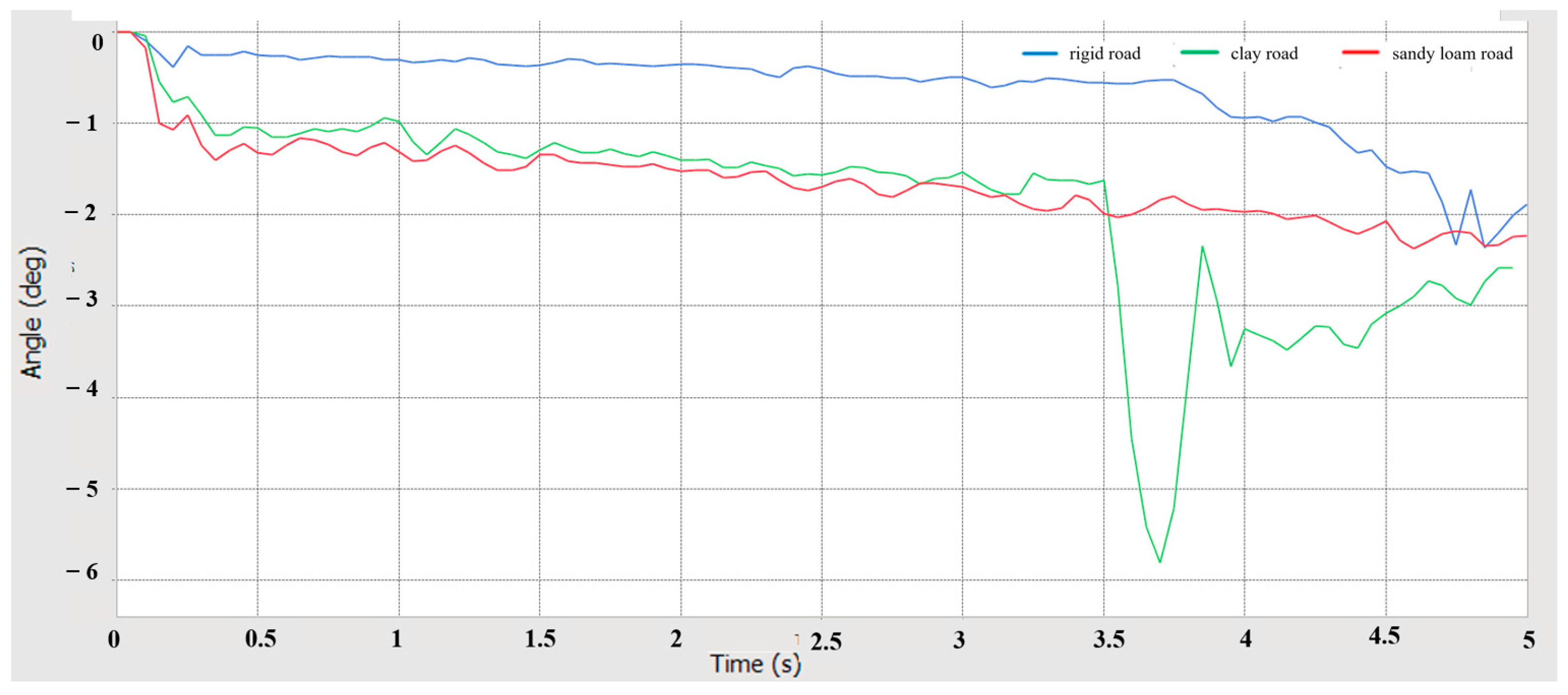
5.2.3. Cross-Slope Driving Simulation Analysis

The prototype may experience dangerous situations such as side-slip and overturn in the cross-slope driving condition. In order to study the stability performance of the prototype under the cross-slope condition, different geological ground models with a slope of 25° are set up to study the dynamical stability of the prototype running under different geologies at the same slope. The traveling speed of the prototype is the same as that of the longitudinal traveling condition, the simulation time is set to 5 s, and the step size is 100. Figure 24 shows the schematic diagram of the prototype traveling in a straight line across the slope.

Figure 25 shows the variation curve of the vibration acceleration of the prototype under different ground conditions. From the simulation analysis, it can be seen that for the prototype in the static equilibrium state, the vibration acceleration fluctuation amplitude is larger, and when the prototype undergoes stable driving, the prototype under different geological conditions experiences center of mass vibration acceleration within different narrow fluctuations near zero, indicating that the cross-slope driving body vibration is small in the prototype under the different ground conditions, with a strong dynamic stability.

Figure 26 shows the variation curve of the lateral inclination angle of the prototype under different ground surface conditions, and the error between it and the inclination angle of the slope is small, which indicates that the prototype does not experience the dangerous condition of tipping over while traveling in a straight line on the cross slope.

By analyzing the data for the longitudinal and cross-slope driving of the prototype, it can be seen that the prototype can stably pass over a 25° slope and adapt to the complex terrain of different soils, and no tipping over phenomenon occurs in the simulation process, which verifies the feasibility of the longitudinal and cross-slope driving of the prototype.

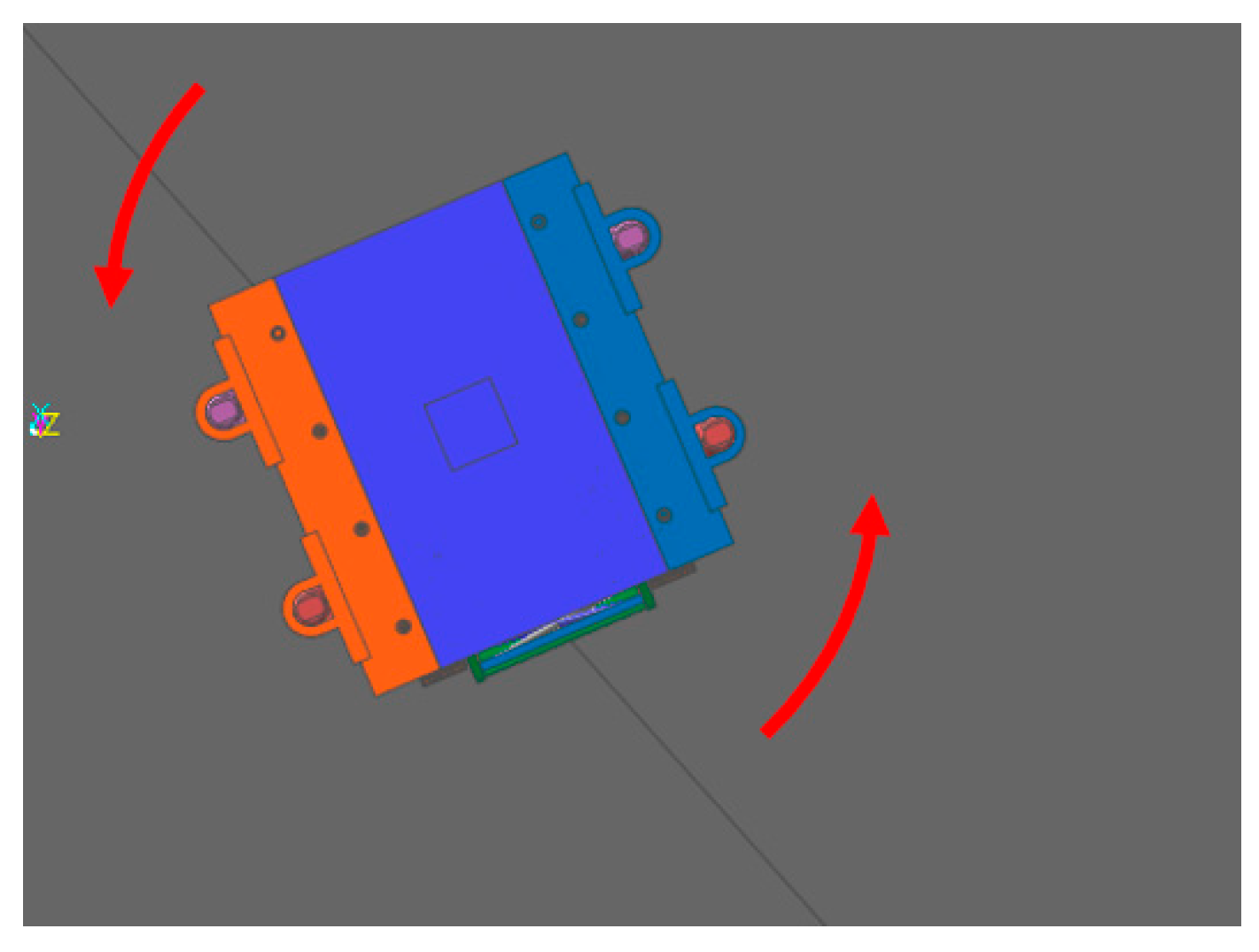
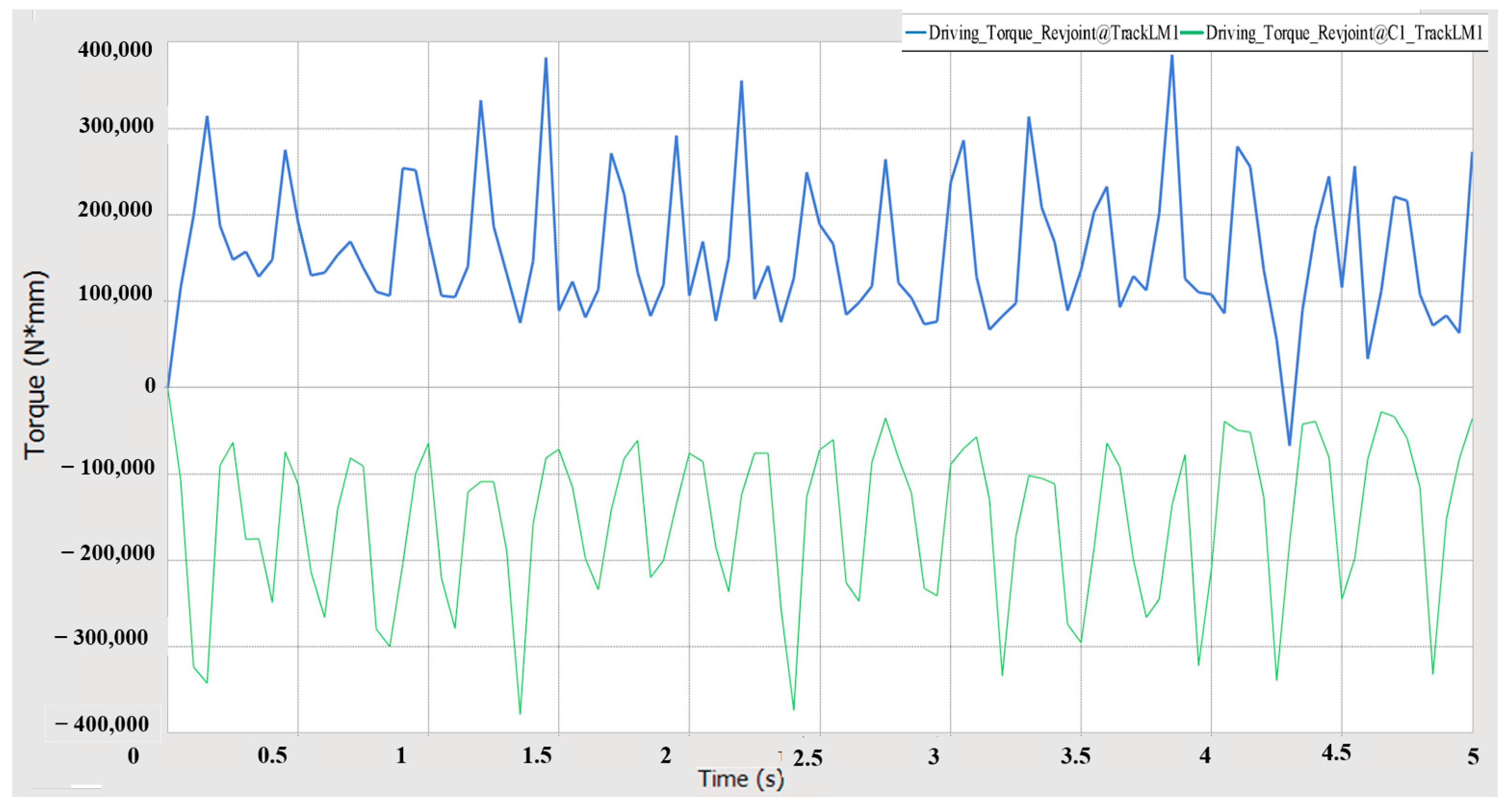
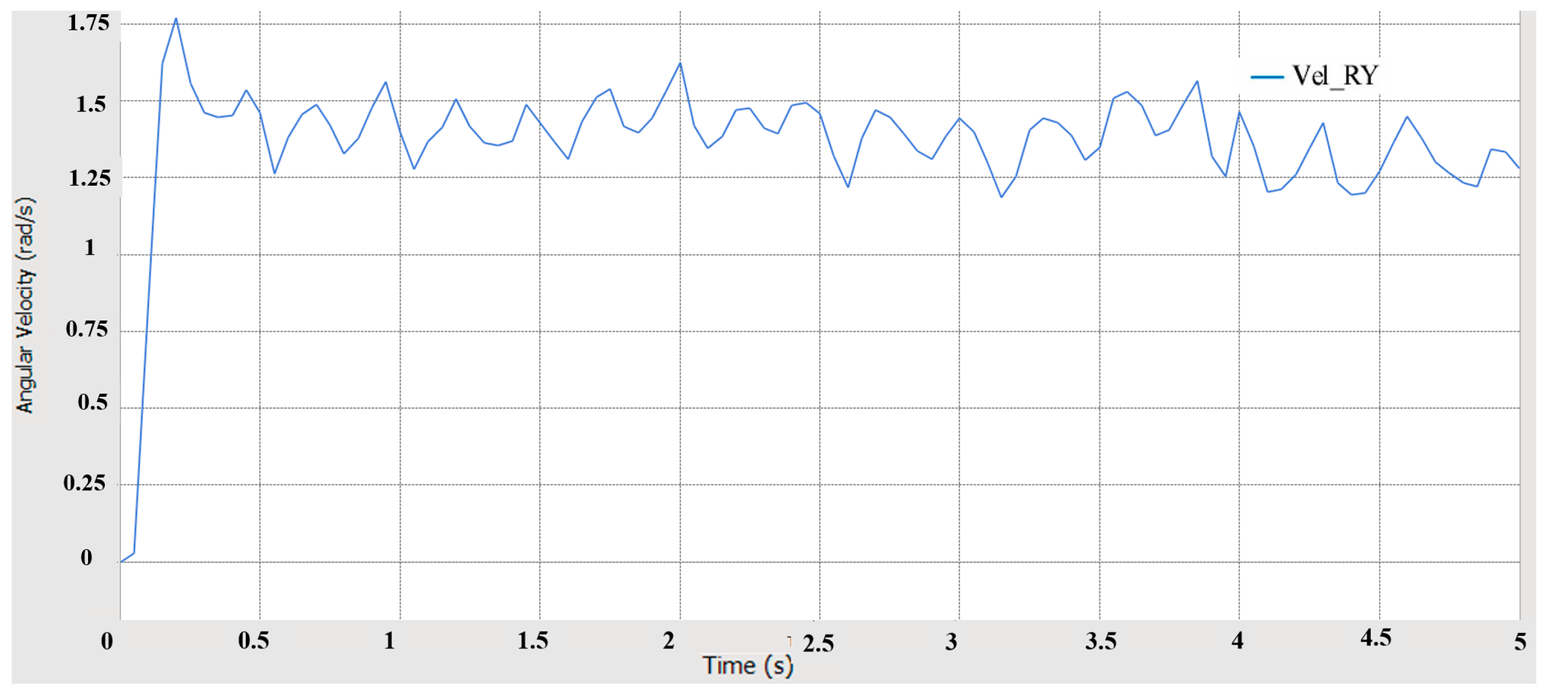
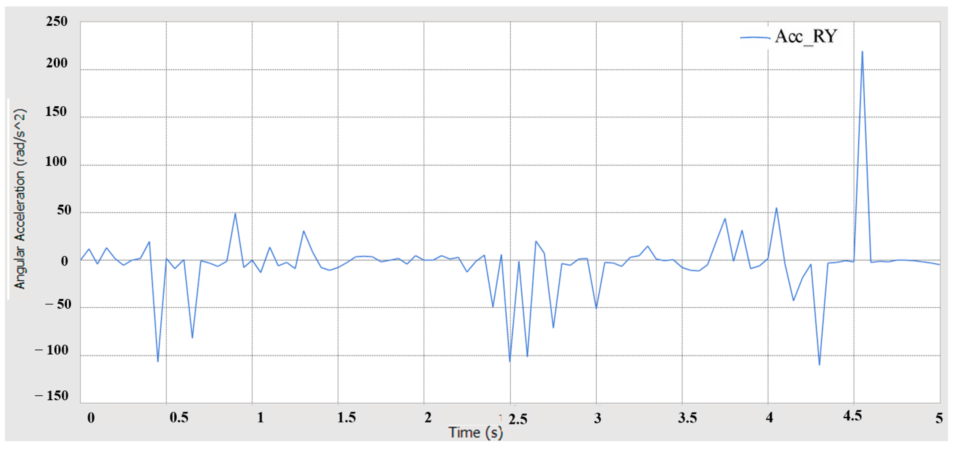
5.3. Steering Performance Simulation Analysis

In the simulation to realize the prototype’s in situ left steering movement, the left side of the track maintains a speed of 2.5 km/h, while the right side moves in the opposite direction at the same speed as the left side. At this time, the turning radius is R = B/2 = 400 mm. The relevant formula is as follows:

$$\left\{\begin{array}{c}{F}_l=\frac{1}{2}mgf-\frac{\mu mgL}{4B}=-1672.13 \mathrm{N}\\ F_r=\frac{1}{2}mgf+\frac{\mu mgL}{4B}=2309.13 \mathrm{N}\end{array}\right.$$

(55)

where $F_l$ and $F$ are the steering resistance on the left and right sides of the track, respectively.

$$\left\{\begin{array}{c}{T}_l=F_{l}r=-165.54 \mathrm{N}\cdot \mathrm{m}\\ T_r=F_{l}r=228.60 \mathrm{N}\cdot \mathrm{m}\end{array}\right.$$

(56)

$$\left\{\begin{array}{c}{P}_l=T_l\omega =1.2 \mathrm{KW}\\ P_r=T_r\omega =1.6 \mathrm{KW}\end{array}\right.$$

(57)

This paper studies the in situ left steering condition of the prototype. During the simulation, the right side of the track’s speed is set to 7 rad/s, and the left side is −7 rad/s. The simulation duration is 5 s, and the step size is 100. Figure 27 shows the schematic diagram of the steering process of the prototype.

Figure 28 shows the change in drive torque on both sides of the prototype during steering. The driving torques of the prototype overlap before the steering motion is performed, and the blue color represents the right side of the track’s braking torque, and the green color represents the left side of the track’s driving torque. A comparison of the simulation results is shown in

Table 3. Comparison of steering driving simulation results.

		Simulation Value	Theoretical Value	Inaccuracy
Driving torque $\mathrm{N}\cdot \mathrm{m}$	Left track	159.64	165.54	3.6%
	Right track	220.72	228.60	3.4%
Driving power $\mathrm{K}\mathrm{W}$	Left track	1.16	1.2	3.6%
	Right track	1.55	1.6	3.4%

.

The stability of the steering process of the prototype was determined by measuring the transverse pendulum angular velocity and transverse pendulum angular acceleration. The smaller the values of transverse pendulum acceleration and transverse pendulum angular acceleration, the more stable the vehicle will be when steering. Figure 29 and Figure 30 show the transverse pendulum angular velocity and angular acceleration of the prototype during steering, respectively. The simulation results show that the prototype in the steering process did not experience a tipping phenomenon, and the prototype can successfully complete the steering movement, as steering driving is more stable, indicating that the design of the ratio between the track grounding length and the track gauge is reasonable, verifying the feasibility of the prototype in steering driving.

5.4. Anti-Rollover Performance Simulation Analysis

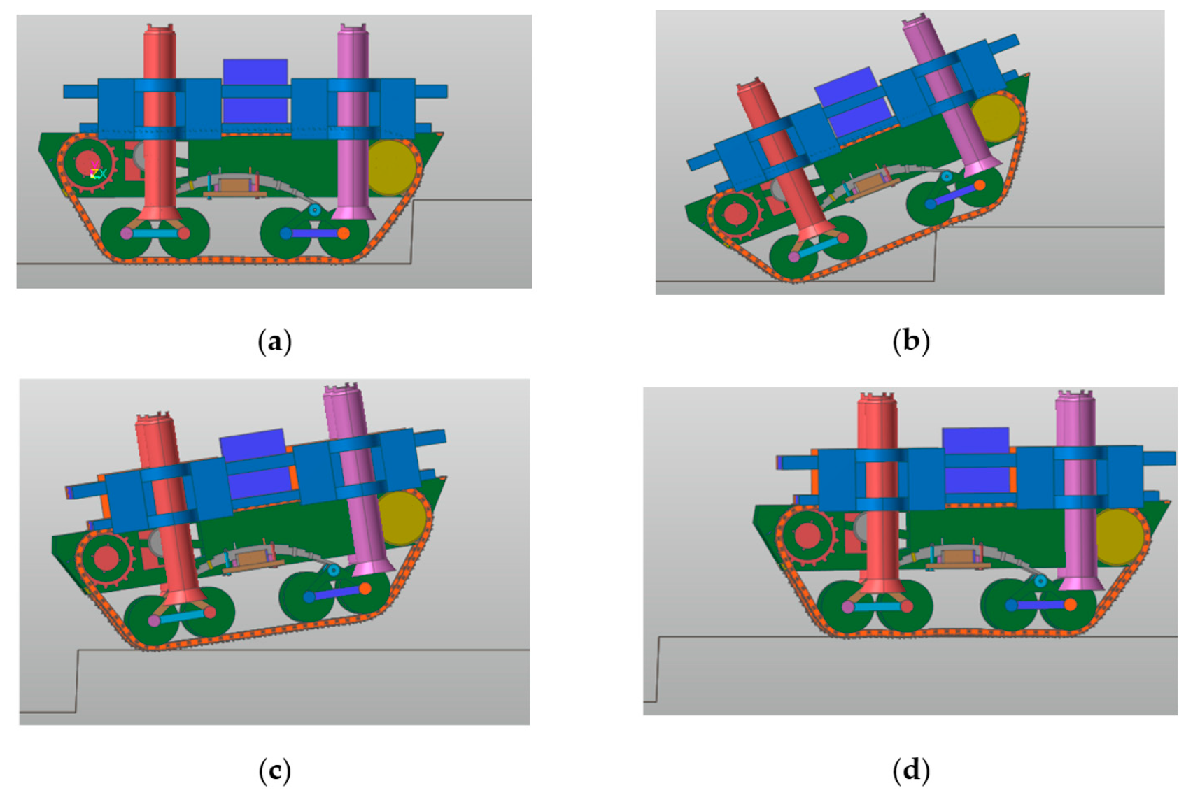
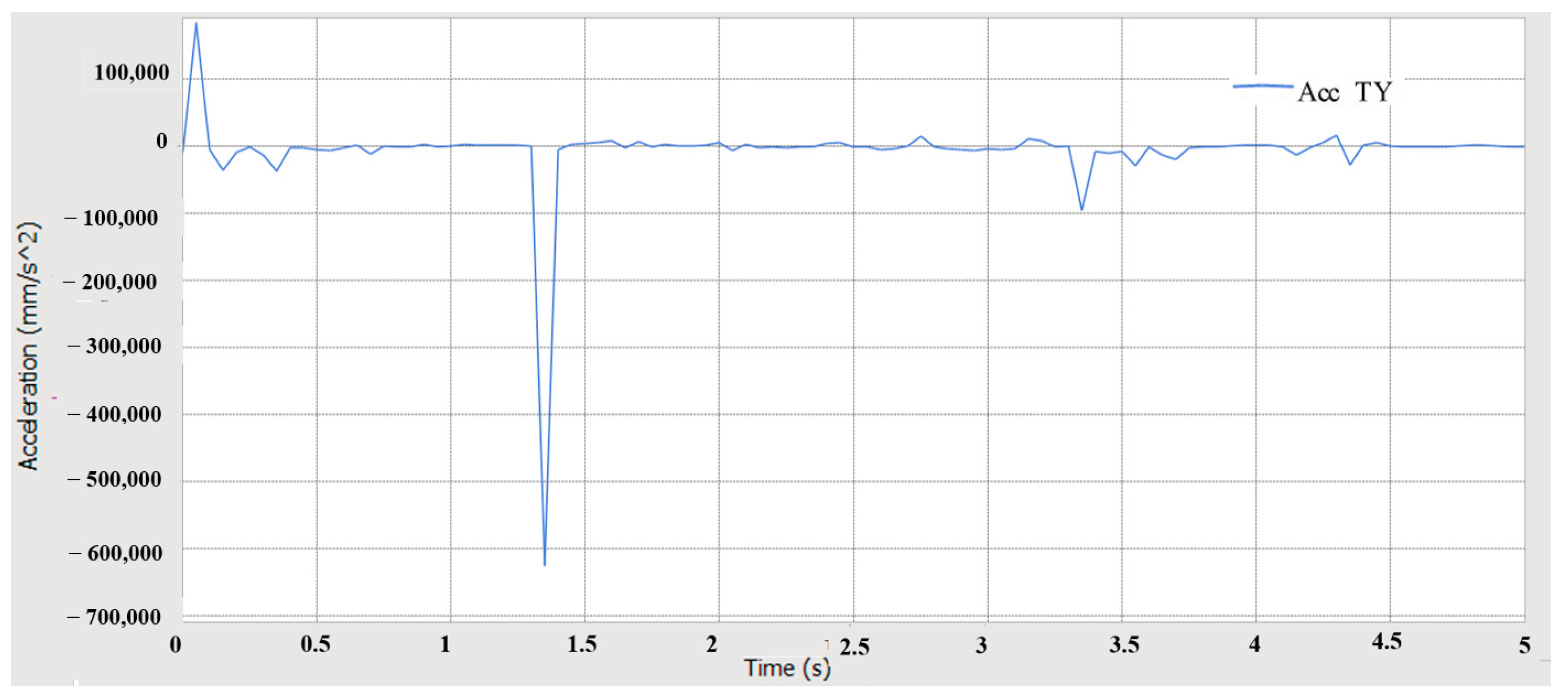
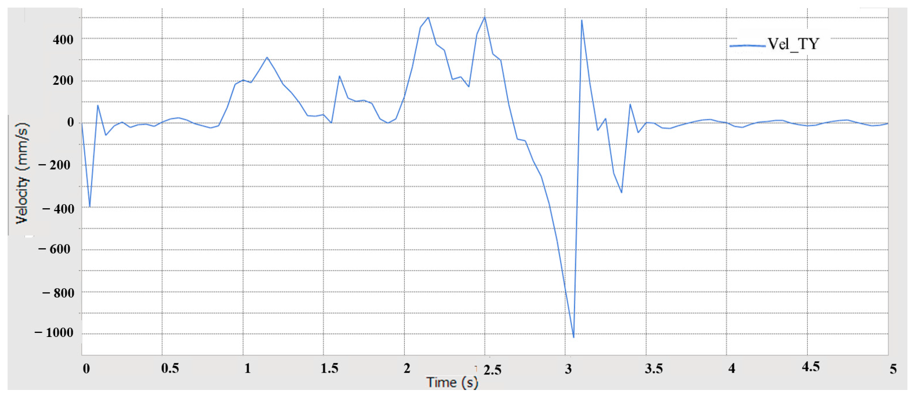
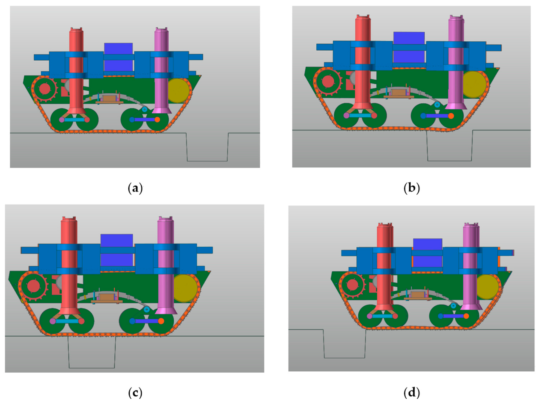
5.4.1. Crossing Obstacles Simulation Analysis

The prototype designed in this paper is required to be able to cross 300 mm obstacles. When the height of the obstacle is 300 mm, the simulation process is shown in Figure 31, which is divided into four processes, namely coming into contact with obstacles, crawling over the obstacles, crossing the obstacles, and completing the obstacle crossing. During the simulation, the traveling speed is set to 2.5 km/h, the simulation time is 15 s, and the step size is 1000.

Figure 32, Figure 33 and Figure 34 show the displacement, acceleration and velocity change curves of the prototype’s center of mass in the vertical direction, respectively. The post-processed data show that the prototype has a small center-of-mass wobble during climbing over the obstacle, and the vibration acceleration is smaller at the smooth moment, indicating that the prototype is able to cross the 300 mm obstacle smoothly.

5.4.2. Over-Groove Simulation Analysis

The prototype designed in this paper is required to be able to cross a 300 mm wide gully. The simulation process of the prototype when the gully is 300 mm wide is shown in Figure 35, which is divided into four processes: preparing to cross the gully, entering the gully, crossing the gully, and completing the crossing of the gully. During the simulation, the traveling speed is set to 2.3 km/h, the simulation time is 15 s, and the step size is 1000.

Figure 36, Figure 37 and Figure 38 show the displacement, acceleration and velocity change curves of the prototype center of mass in the vertical direction when passing over the gully, respectively. From the post-processing analysis, it can be seen that there is a 20 mm fluctuation in the displacement component of the center of mass in the vertical direction when the prototype passes over the gully; at the same time, the fluctuation of the acceleration and velocity of the center of mass in the vertical direction is small, which indicates that the prototype passes through the gully with a small amplitude of body swaying, and it can pass smoothly over the gully with a width of 300 mm, and the through performance is good.

The data analysis shows that the prototype can stably pass over obstacles with a height of 300 mm and over gullies with a width of 300 mm, which verifies the feasibility of the prototype to cross obstacles and cross gullies.

6. Conclusions

Aiming at the problems of low production efficiency and a low safety factor in coal mines, a new type of support equipment was designed. Through driving theory analysis, kinematics and dynamics analysis and modeling, RecurDyn multi-body dynamics software [21] was used to conduct simulation research on it, simulation curves under different working conditions were obtained, and the simulation results and theoretical analysis results were mutually verified. The main results are as follows.

(1)

The theoretical feasibility foundation of the prototype was laid through the driving theory analysis of the prototype. In the design, the height of the prototype center of mass should be reduced as far as possible to ensure that $L_1,L_2>B$ .

(2)

The kinematics analysis of the prototype was carried out, and the position coordinates at different times were analyzed using the RPY angles. The space coordinate system of the prototype was established, and the position coordinates of the prototype at different times were solved by establishing the plane kinematics equation.

(3)

By using the discrete body dynamic model method, the track was concentrated as the mass block, a 14-degree-of-freedom dynamic system model was established which can reflect the longitudinal dynamic characteristics of the driving system of the prototype, and the differential equation of motion was established by using the Lagrange dynamic equation method, which provides a theoretical basis for the dynamic simulation.

(4)

Using RecurDyn multi-body dynamics simulation, the results verify that the prototype has good driving performance, conforms to the anti-roll design, has good steering performance, has good passing performance, and has good ride comfort and dynamic stability.

The research results of this paper realize the mechanization, automation and high efficiency of coal mine production, realize safe underground production, and provide an effective solution to ensure the sustainable development of coal resources and the safety of coal mine production. In future research, it is necessary to put this prototype into production and carry out field tests to identify its shortcomings and further improve the design. This is also the direction of our future efforts.

References

1. Du, Y.P. Quantitative Analysis of Economic and Safety Benefits of Coal Mining Mechanization in China’s Coal Industry. Master’s Thesis, China University of Mining and Technology, Xuzhou, China, 2022. [Google Scholar]
2. Zhang, L.X.; Wang, Y.M.; Yang, W.J. Design and research on mechanical arm of automatic handling equipment for hydraulic pillars. J. Coal Technol. 2022, 41, 224–227. [Google Scholar]
3. Zhou, K.; Wang, Q.; Tang, J.N. Tripartite Evolutionary Game and Simulation Analysis of Coal Mining Safe Production Supervision under the Chinese Central Government’s Reward and Punishment Mechanism. Math. Probl. Eng. 2021, 2021, 5298890. [Google Scholar] [CrossRef]
4. Hou, L.Q. Problems and countermeasures in coal mine tunneling support. J. Energy Energy Conserv. 2023, 212, 202–204. [Google Scholar]
5. Ivan, S.; Svitlana, S.; Alla, S. Field investigations of deformations in soft surrounding rocks of rocks of roadway with roof-bolting Supports by auger mining of thin coal seams. Rud.-Geol.-Naft. Zb. 2022, 37, 23–38. [Google Scholar]
6. Shahzad, M.; Majeed, Y.; Emad, M.Z.; Arshad, M.; Goraya, R.; Akram, M. Assessing mechanical characteristics of typical support system being used in thin seam coal mining of Pakistan. Int. J. Min. Miner. Eng. 2022, 13, 333–351. [Google Scholar] [CrossRef]
7. Xue, T.L.; Zhang, X.H.; Du, D.T. Developing History and Trend of Mine Support Equipment in China. Appl. Mech. Mater. 2010, 42, 42. [Google Scholar] [CrossRef]
8. Li, J. Program design and performance study of self-moving support equipment. Electron. Technol. Softw. Eng. 2023, 246, 108–111. [Google Scholar]
9. Bruzzone, L.; Nodehi, S.E.; Fanghella, P. Tracked Locomotion Systems for Ground Mobile Robots: A Review. Machines 2022, 10, 648. [Google Scholar] [CrossRef]
10. Purdy, D.J.; Simner, D. A brief investigation into the effect on suspension motions of high unsprung mass. J. Battlef. Technol. 2004, 7, 15–20. [Google Scholar]
11. Hetherington, J.G. Scale—Model testing of soil—Vehicle systems. J. Battlef. Technol. 2004, 7, 7–10. [Google Scholar]
12. Purdy, D.J.; Kumar, R.J. Mathematical model ling of a hydro-gas suspension unit for tracked military vehicles. J. Battlef. Technol. 2005, 8, 7–14. [Google Scholar]
13. Song, F.H.; Yan, C.C.; Sun, J.B. Analysis of the key points of top plate management in high-grade general mining working face. Inn. Mong. Coal Econ. 2016, 217, 51–78. [Google Scholar]
14. Kleppner, D.; Kolenkow, R. An Introduction to Mechanics; Cambridge University Press: Cambridge, UK, 2013. [Google Scholar]
15. Uicker, J.J.; Pennock, G.R.; Shigley, J.E. Theory of Machines and Mechanisms, 5th ed.; Oxford University Press: Oxford, UK, 2016. [Google Scholar]
16. Wei, D. Design of Electric Control System of Fully Hydraulic Driven Crawler Tractor; Northwest A&F University: Xianyang, China, 2013. [Google Scholar]
17. Solidworks.com. Available online: https://www.solidworks.com/zh-hans (accessed on 20 September 2023).
18. Ji, G.X. Design and Motion Performance Analysis of Tracked Manned Lunar Rover Mobile System; Harbin Institute of Technology: Harbin, China, 2013. [Google Scholar]
19. Ou, Y. Design and Analysis of Mechanical System of Special Ground Mobile Robot; Nanjing University of Science and Technology: Nanjing, China, 2013. [Google Scholar]
20. Yao, J.Q. Study on the Dynamics of Crawler System of Longitudinal Tunnel Header; Liaoning Technical University: Fuxin, China, 2012. [Google Scholar]
21. Recurdyn.cn. Available online: https://www.recurdyn.cn/ (accessed on 20 September 2023).
Figure 1. Hydraulic strut structure diagram of double movable column.
Applsci 13 10613 g001
Figure 2. MSES virtual prototype structure.
Applsci 13 10613 g002
Figure 3. The three views of the prototype: (a) the main view of the prototype; (b) the side view of the prototype; (c) the top view of the prototype.
Applsci 13 10613 g003
Figure 4. Schematic diagram of prototype forces.
Applsci 13 10613 g004
Figure 5. The prototype driving uphill and downhill: (a) prototype uphill driving; (b) prototype downhill driving.
Applsci 13 10613 g005
Figure 6. Prototype traveling sideways.
Applsci 13 10613 g006
Figure 7. Prototype driving over obstacles.
Applsci 13 10613 g007
Figure 8. Prototype driving over the groove: (a) front support wheel over groove; (b) rear support wheel over groove.
Applsci 13 10613 g008
Figure 9. Prototype kinematic coordinate system: (a) prototype kinematic coordinate system; (b) prototype planar kinematic model.
Applsci 13 10613 g009
Figure 10. Longitudinal dynamics model of prototype driving system.
Applsci 13 10613 g010
Figure 11. Driving condition of the loaded prototype travelling in a straight line along a flat road.
Applsci 13 10613 g011
Figure 12. Prototype drive torque trend.
Applsci 13 10613 g012
Figure 13. Velocity change curve of the prototype in each direction.
Applsci 13 10613 g013
Figure 14. Climbing driving condition of the loaded prototype at 25° slope.
Applsci 13 10613 g014
Figure 15. Driving speed curve of the prototype on different slopes.
Applsci 13 10613 g015
Figure 16. Driving acceleration curves of the prototype on different slopes.
Applsci 13 10613 g016
Figure 17. Driving speed curves of the prototype under different ground conditions.
Applsci 13 10613 g017
Figure 18. Climbing pitch angle of the prototype under different ground conditions.
Applsci 13 10613 g018
Figure 19. Driving torque of the prototype under different ground conditions.
Applsci 13 10613 g019
Figure 20. Driving conditions of the loaded prototype travelling downhill.
Applsci 13 10613 g020
Figure 21. Driving speed of the prototype under different road surface conditions.
Applsci 13 10613 g021
Figure 22. Vertical acceleration of the prototype under different road surface conditions.
Applsci 13 10613 g022
Figure 23. Pitch angle of the prototype on different surfaces.
Applsci 13 10613 g023
Figure 24. Driving condition of the loaded prototype travelling in a straight line on a cross slope straight line.
Applsci 13 10613 g024
Figure 25. Vertical acceleration of the prototype under different ground surfaces.
Applsci 13 10613 g025
Figure 26. Lateral inclination of the prototype at different ground levels.
Applsci 13 10613 g026
Figure 27. Prototype load leveling steering condition.
Applsci 13 10613 g027
Figure 28. Driving wheel torque on both sides of the prototype.
Applsci 13 10613 g028
Figure 29. Prototype traverse angular velocity.
Applsci 13 10613 g029
Figure 30. Prototype pendulum angular acceleration.
Applsci 13 10613 g030
Figure 31. Prototype load crossing simulation: (a) contact with an obstacle; (b) climbing over an obstacle; (c) overcoming an obstacle; (d) completion of obstacle crossing.
Applsci 13 10613 g031
Figure 32. Vertical displacement of the prototype.
Applsci 13 10613 g032
Figure 33. Vertical acceleration of the prototype.
Applsci 13 10613 g033
Figure 34. Velocity of prototype in vertical direction.
Applsci 13 10613 g034
Figure 35. Prototype load over groove simulation condition: (a) prepare to cross the groove; (b) enter the groove; (c) cross the groove; (d) completion of groove crossing.
Applsci 13 10613 g035
Figure 36. Vertical displacement of the prototype.
Applsci 13 10613 g036
Figure 37. Vertical acceleration of the prototype.
Applsci 13 10613 g037
Figure 38. Velocity of the prototype in the vertical direction.
Applsci 13 10613 g038