Abstract
Accurate predictions of radio frequency electromagnetic field (RF-EMF) levels can help implement measures to reduce exposure and check regulatory compliance. Therefore, this study aims to predict the RF-EMF levels in the medium using an artificial neural network (ANN). The work was conducted at Ondokuz Mayis University, Kurupelit Campus, where the measurement location has line-of-sight to the base stations. Band selective measurements were also performed to assess the contribution of 2G/3G/4G services to the total RF-EMF level, which was found to be the highest among all services within the total band. Long-term RF-EMF measurements were carried out for 35 days within the frequencies of 100 kHz to 3 GHz. Then, an ANN model with Levenberg–Marquardt (LM) and Bayesian Regulation (BR) algorithms was proposed, which utilized inputs from real-time RF-EMF measurements. The performance of the models was assessed in terms of mean squared error (MSE) and regression performance. The average MSE and regression performances of the models were similar, with the lowest testing MSEs of 2.78 × 10⁻³ and 3.76 × 10⁻³ for LM and BR methods, respectively. The analysis of the models showed that the proposed models help to predict the RF-EMF level in the medium with up to 99% accuracy.
1. Introduction
Base stations serve a limited number of users in a localized geographical area. As users demand more multimedia applications that require high data rates, the number of base stations increases. Each base station utilizes a specific communication technology, such as GSM (Global System for Mobile Communications), UMTS (Universal Mobile Telecommunications System), or LTE (Long Term Evolution). The coverage area for base stations using GSM technology is relatively large (e.g., 10 km), but it is much smaller for LTE base stations (e.g., 1 km). Compared to GSM base stations, many more LTE base stations need to be installed in order to serve the same coverage area [1]. As the LTE system supports high data rate applications, the number of LTE base stations around us is rapidly increasing to meet the growing demand of users. Because each base station establishes a connection with users in its coverage area through electromagnetic waves, the increasing number of base stations also increases the amount of electromagnetic fields they emit. Hence, measuring and evaluating the radio frequency electromagnetic field (RF-EMF) values emitted by base stations is crucial to protect human beings from potential harmful effects. For instance, [2] classified RF-EMF as possibly carcinogenic to humans. In [3], it was indicated that electromagnetic fields pose health risks that extend beyond cancer, including conditions like electromagnetic hypersensitivity. In [4], it was shown that low-level EMF at 2.45 GHz causes an increase in inflammation, testicular damage, and has a negative impact on male reproductive system function. The work of [5] indicated that oxidative stress induced by RF-EMF can lead to DNA damage in neurons, while [6] suggested that higher brain exposure to RF-EMF is related to lower non-verbal intelligence but not to other cognitive function outcomes. As indicated in [7], to estimate the risk for human health by RF-EMF exposure experimental studies in humans and epidemiological studies still need to be considered. Many international organizations, such as the World Health Organization (WHO), the International Commission on Non-Ionizing Radiation Protection (ICNIRP), the Institute of Electrical and Electronics Engineers (IEEE), and the Federal Communications Commission (FCC), study the potential effects of electromagnetic fields on human health.
Each country has its own limit values for exposure to electromagnetic fields. In Turkey, the Information and Communication Technologies Authority (ICTA) is authorized to set limit values, and it adopts 70% of the limit values determined by ICNIRP. Table 1 shows the limit values for the total electric field strength (E) of the environment between 10 kHz–94,000 MHz, as determined by the ICNIRP [8] and the ICTA [9]. For example, the ICNIRP limit value for base stations using the 900 MHz frequency is 41.25 V/m, whereas ICTA’s limit value is 28.80 V/m. Similarly, for base stations using the 2100-MHz frequency for 3G, the ICNIRP’s limit value is 61 V/m, and the ICTA’s limit value is 42.93 V/m. The limit values for 4G base stations using the 2600 MHz frequency band are also 61 V/m and 42.93 V/m for the ICNIRP and the ICTA, respectively.

Table 1.
Limit E levels.
Studies on the measurement and evaluation of RF-EMF levels from a base station mainly focus on short-term, long-term, and band-selective RF-EMF measurements. Studies [10,11,12,13,14] evaluate the short term, [15,16,17,18] assess long-term, and [19,20,21] provide short-term, band-selective RF-EMF measurement results for different mediums.
Short-term RF-EMF measurements may not always be sufficient for evaluating the levels in an environment. Since RF-EMF values can vary throughout the day, recorded values may differ depending on the measurement time. Therefore, at least one daily RF-EMF dataset is necessary to analyze levels in an environment. Long-term RF-EMF measurements, other than one day, are of great importance for modeling and analyzing variations. However, conducting long-term measurements can be very costly, both in terms of time and equipment. Therefore, modeling RF-EMF changes in a location with the least time and cost is crucial.
1.1. Related Works
Recently, neural networks have been successfully applied to predict electric and magnetic field levels, as well as signal power loss. In [22], a novel artificial neural network (ANN)-based indoor electric field strength prediction model was presented, while an outdoor prediction model for both a macrocell [23] and microcell [24] mobile radio environment was proposed. A spatial electric field strength prediction using a hybrid wavelet-neural model was presented in [25]. Electric field strengths were obtained through drive-test measurements, and a new generalized regression neural network model was created to predict power loss. In [26], a hybrid autoregressive integrated moving average and neural network model were used to predict electric field levels along with the buildings close to digital television transmitters. Computed and measured received signal strengths were compared, which were shown to be reasonably close. Electric [27] and magnetic field [28] estimation was performed under/near high voltage transmission and distribution lines using ANN, and the electric and magnetic field levels were predicted accurately. Indoor wideband electric field radiation was predicted in [29] using the combined wavelet transform and time series analysis-based method. The better prediction accuracy performance of the proposed method was proved by the comparison of the results obtained by non-hybrid methods. In [30], RF-EMF values were assessed with the use of a four-frequency-bands RF sensor. Potential RF-EMF exposure hotspots were determined in a very large geographical area and time-series clustering, and spatiotemporal interpolation techniques were proposed to improve the spatiotemporal assessment of RF-EMF exposure. RF-EMF exposure levels in an outdoor urban environment were predicted in [31,32] using drive test measurement results and both fully connected and hybrid-connected ANN models. In [33], electric field levels were measured in the dense areas, and ANN models were created to predict electric field values in random locations of a university campus; the prediction accuracy of models was compared.
1.2. Existing Gaps in Related Works
Although there are studies on predicting solely electric and magnetic field levels using ANN, the modeling and prediction of total RF-EMF levels within the cellular frequency bands are less studied. Therefore, besides providing a realistic idea about the RF-EMF levels in the medium, this study aims to predict RF-EMF levels using proposed ANN models that are created based on experimental measurement results. To reach this goal first, extensive RF-EMF level measurements were performed within the band 100 kHz–3 GHz at Ondokuz Mayıs University, Kurupelit Campus, for five weeks and saved for future processing. Then, the contribution percentages of the services within the band to the total RF-EMF levels were determined, and the measurement data were analyzed in detail.
This study provides several contributions as follows:
- A new ANN model with Levenberg–Marquardt (LM) and Bayesian Regulation (BR) learning algorithms was proposed.
- The proposed models were used to predict RF-EMF levels and determine long-term exposure patterns without real-time measurements.
- A performance comparison was made with similar works, and it was shown that the proposed models have higher prediction accuracy.
Therefore, the use of the proposed models for predicting RF-EMF levels leads several benefits, such as:
- Mitigating potential health risks by implementing measures to reduce exposure to RF-EMF.
- Helping regulatory compliance by identifying areas where the maximum allowable levels are likely to be exceeded.
- Supporting the research and development of new technologies that utilize RF-EMF and helping test the effectiveness of new technologies in reducing RF-EMF exposure.
2. Artificial Neural Networks
ANN models are machine learning algorithms designed to emulate the functions of the human brain. The algorithm is composed of artificial units called neurons, which are interconnected processing nodes. These models are frequently preferred for creating highly suitable mathematical models for learning and predicting system modeling in engineering applications. An MLP is the most widely used ANN with three layers of input, hidden, and output (Figure 1). The inputs are sent to the hidden layer through the input layer for processing. In the hidden layer, weights are calculated and updated according to targets using different activation functions. The output layer obtains the prediction results [34].
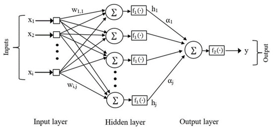
Figure 1.
The MLP architecture with a single hidden layer and one output layer.
In the figure, ith input of the network is xi, the weights connecting the ith input to the jth hidden neuron are wij, and the output of the jth hidden neuron is hj, which can be calculated through (1).
In the equation, f shows the activation function. The output of the network is calculated using (2), in which αj is the weight of the connection between the jth hidden neuron and the output.
The weights are changed in the training session to obtain the desired output. The MSE between the output of the actual outputs (yk) and network outputs () is calculated using (3).
where N is the number of observations. In ANNs, backpropagation algorithms are used to reduce prediction error.
The LM algorithm is used to solve nonlinear least squares problems and combines the gradient descent and the Gauss–Newton methods. The algorithm uses the advantage of both methods and chooses the one according to closeness to the optimal value. The iterative training algorithm makes LM faster than other training algorithms [35].
The BR training algorithm can decrease the need for cross-validation processes. In BR, nonlinear regression is transformed into a statistical structure that yields an advantage of high functionality. Because of the Bayesian criterion used, overtraining is prevented, and overfitting is also restrained owing to the elimination of invalid parameters and weights [35].
With LM and BR, lower MSEs are obtained; thus, they are widely used. When using these algorithms, the memory usage and processing time must be considered. The data type is also decisive in the selection of algorithms, e.g., BR outperforms LM for noise data but has a larger processing time.
3. Methodology
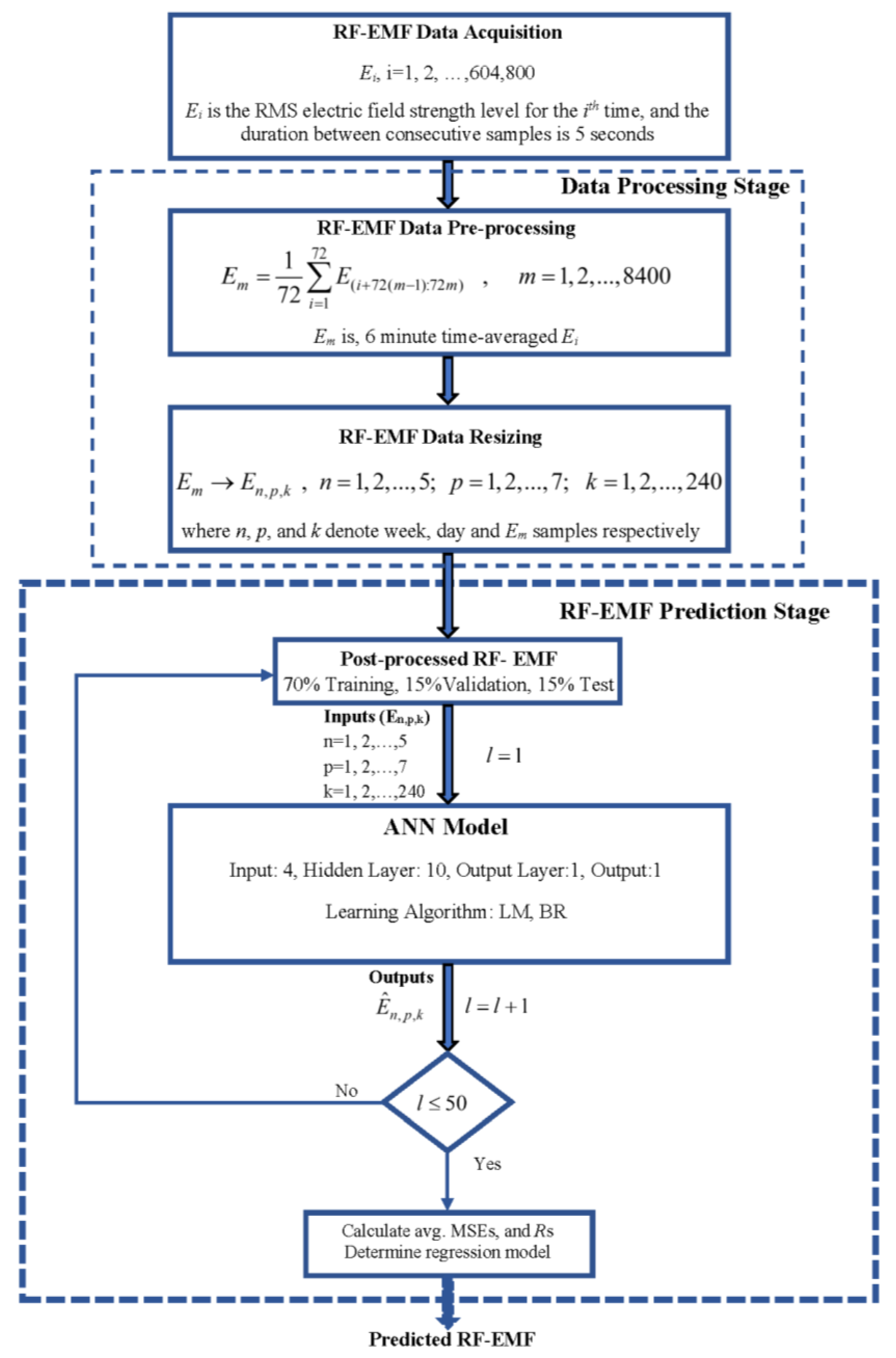
The methodology of this study consists of three main stages, as illustrated in Figure 2. In the figure, 604,800 refers to the number of electric field strength data recorded at 5-s intervals for 5 weeks (35 days). In addition, 72 were the data recorded at 5-s intervals corresponding to 6 min. Also, 8400 represents the number of electric field strength data averaged over 35 days and 6 min. Furthermore, 240 refers to the number of electric field strength data averaged over 1 day and 6 min. n denotes the week index, ranging from 1 to 5, and p denotes day index from 1 to 7. k is the 6 min averaged electric field intensity over a day with values between 1 and 240, and l is the number of times the network trained. The first stage involves the measurement of RF-EMF data, the second stage involves the processing of measurement data, and the third stage involves the creation of the RF-EMF prediction model. The details of each stage are provided in the following sections.
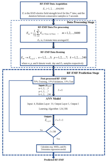
Figure 2.
Diagram of RF-EMF prediction model.
3.1. RF-EMF Data Acquisition
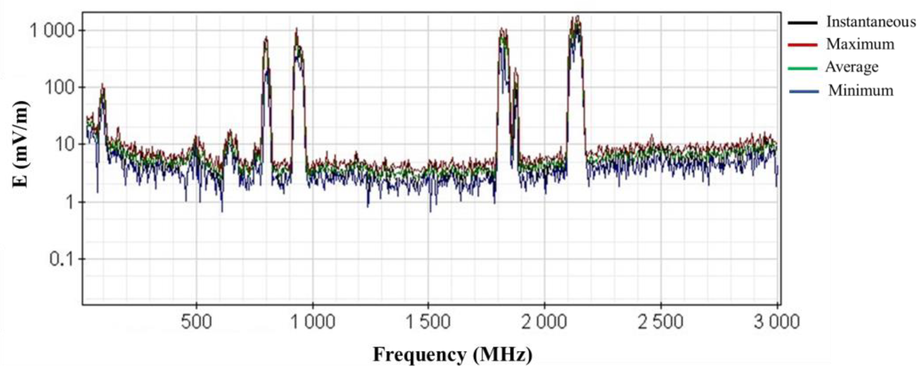
Measurements were conducted to determine the percentage of the total RF-EMF level in the environment that originates from base stations; general and statistical characteristics were obtained. Band-selective RF-EMF measurements were made using the Narda SRM-3600 EMF meter with a 3501/03 isotropic electric field probe [36]. The mathematical details of the measurements can be found in [16]. Figure 3 shows an example of a spectrum taken in the measurement environment using the Narda SRM-3600, which covers 23 services from the low band (27 MHz–87.5 MHz) to ETC6 (2.67 GHz–3 GHz). The contributions of each service in the spectrum to the total RF-EMF were determined and presented in Table 2. The results reveal that LTE 800 (4G), GSM 900 (2G), GSM 1800 (2G), and UMTS 2100 (3G) services account for 99.32% of the total RF-EMF in the environment, with the highest contribution being from the UMTS 2100 service at 34.99%. It can be concluded from Table 2 that the RF-EMF value at the measurement location is generated by base stations from 2G, 3G, and 4G services.
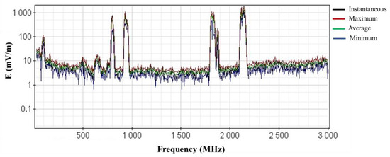
Figure 3.
An example of 27 MHz–3 GHz spectrum measurement.
Table 2.
Contributions of services to RF-RMF at measurement location.
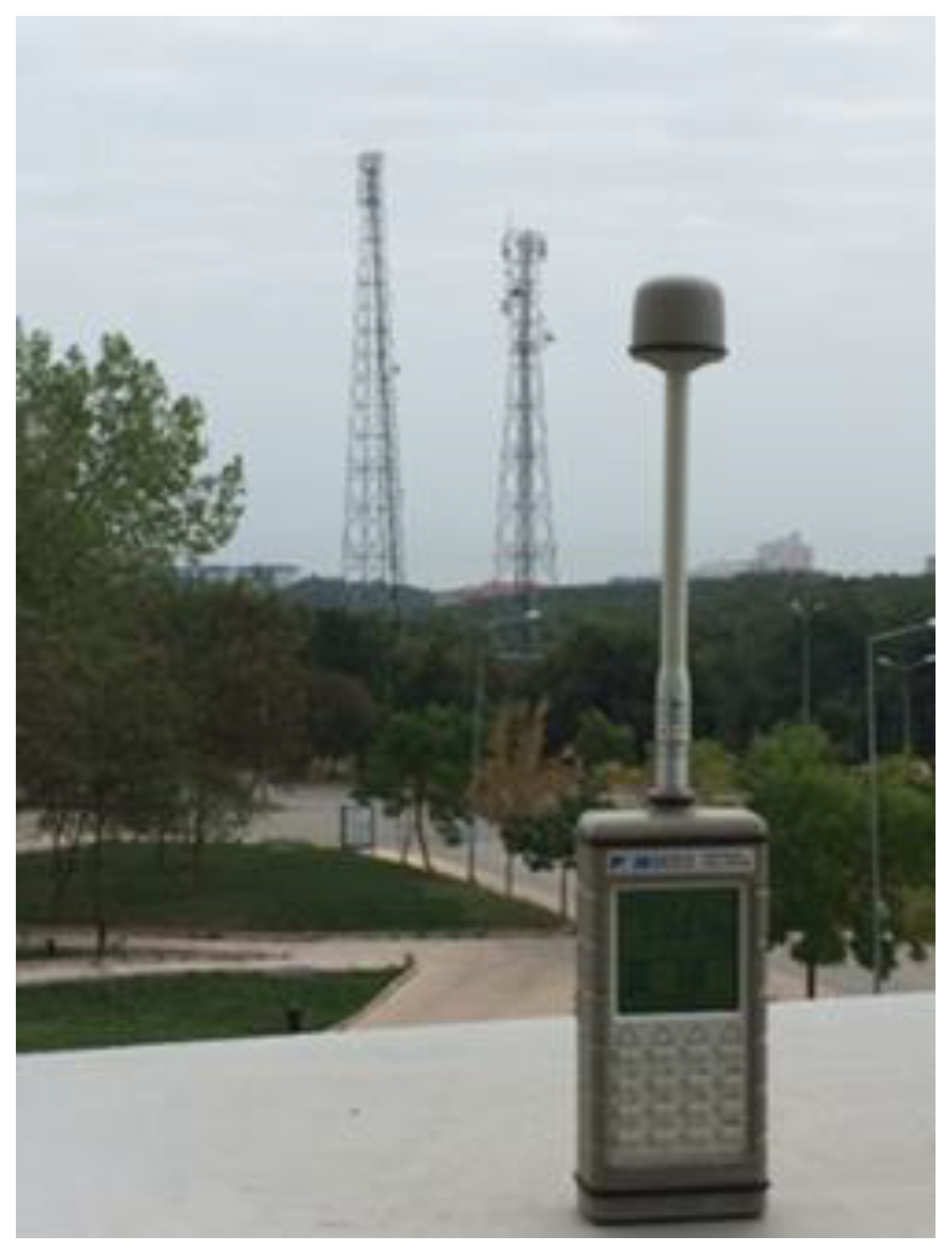
In this study, RF-EMF measurements were performed on a suburban campus during five weeks of the fall semester (35 days in total), when there are many active users of the base stations, in a location that directly sees (Figure 4) the base stations. The line-of-sight path length is ~100 m, and technical specifications of the base stations are as given in [37]. The PMM 8053 EMF meter with an EP-330 isotropic probe was used to measure the instantaneous RMS electric field strength (Ei) in the frequency band of 100 kHz to 3 GHz. The duration between consecutive samples is five seconds.
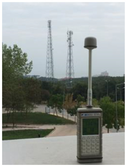
Figure 4.
Long-term RF-EMF measurement setup.
3.2. Data Processing
During the five-week period of measurements, a total of 604,800 Ei values were recorded. Long-term daily measurements were started at 06:00 in the morning and ended at 06:00 the next day. Six-minute averages were used according to the ICNIRP’s guidelines. Because samples were taken every 5 s, a total of 72 samples were taken in 6 min. The time-averaged electric field strength (Em) was calculated as in (4).
where m represents the total number of time-averaged data index.
The Em was reshaped to include the Em samples (k) for each day (p) of the weeks (n) as given in (5).
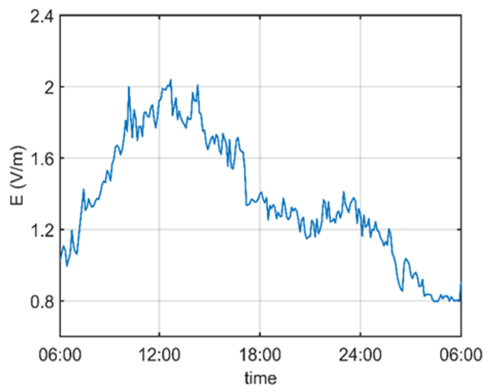
The change in RF-EMF level for Monday, the first day of the measurements (E1,1,k), is given in Figure 5 as an example of En,p,k. As seen from the figure, the maximum RF-EMF level recorded is 2.04 V/m. This value is well below 21 V/m, which is the lowest limit value between 100 kHz–3 GHz determined by ICTA. The mean value of the RF-EMF level is 1.3716 V/m, and the standard deviation is 0.3381 V/m. Additionally, the RF-EMF values measured in the morning (between 06:00–07:00) and at night (between 24:00–06:00) are quite low compared to the noon hours. The RF-EMF value measured at noon (e.g., 2.04 V/m) is almost 2.5 times higher than the value measured in the morning (e.g., the minimum RF-EMF value measured at 0.81 V/m). Because the measurements were made at the OMU Kurupelit Campus (Samsun, Turkey), Figure 5 shows a significant decrease in the measured RF-EMF value after 17:30 when students start to leave the campus.
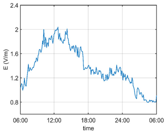
Figure 5.
Daily RF-EMF levels (for Monday).
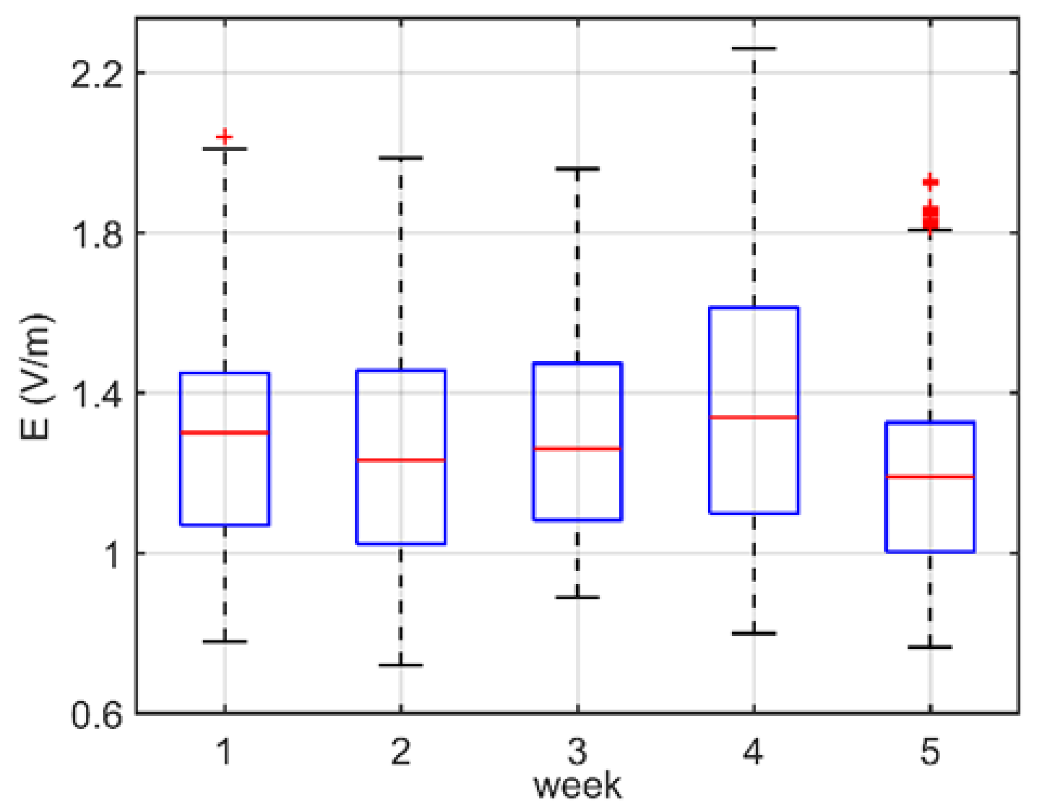
The RF-EMF measurement results of each week (five weeks in total) are given in Figure 6. As can be concluded from the figure, there are differences in RF-EMF levels not only at different times of the day but also between working and nonworking days. The one-week-long measurement data show RF-EMF data starting at 06:00 on Monday morning and continuing until 06:00 on Monday morning the following week. The statistical evaluations of weekly measurements are given in Figure 7. In figure, red lines indicate the medians, the bottom and top edges of the blue boxes indicate the 25th and 75th percentiles, and red plus signs illustrate the outliers. The mean RF-EMF value for the first week is 1.2757 V/m, and the mean values for the second, third, fourth, and fifth weeks are 1.2513 V/m, 1.2849 V/m, 1.3880 V/m, and 1.1968 V/m, respectively. Additionally, the outliers in the data from the fifth week may be due to exams held on campus.
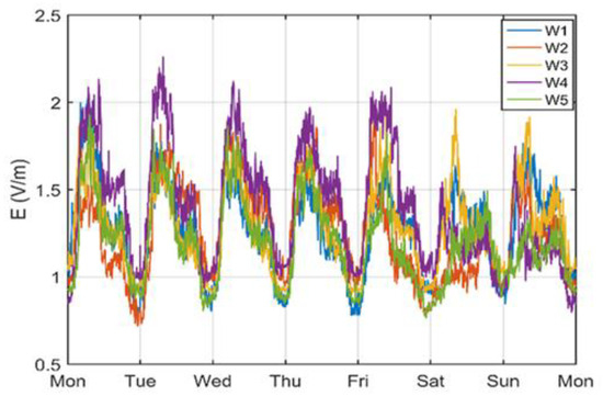
Figure 6.
Daily variation of RF-EMF levels for five weeks.
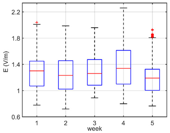
Figure 7.
Statistical analysis of weekly RF-EMF data.
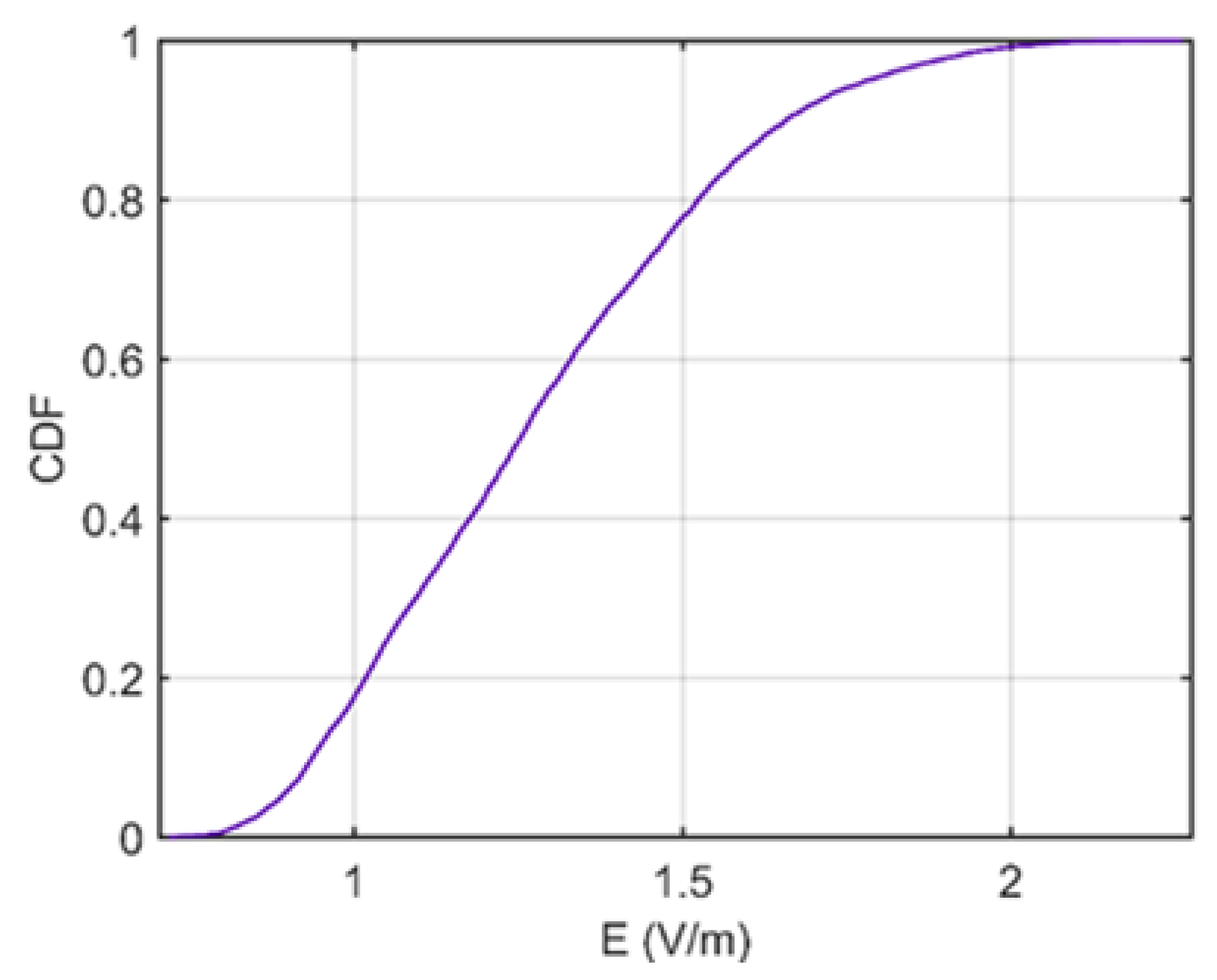
The generalized cumulative distribution function of all five weeks’ RF-EMF data is given in Figure 8. As can be seen from Figure 8, 50% of the measured RF-EMF values are below 1.2528 V/m, while they are lower than 1.6571 V/m for 90% of the measurement data.

Figure 8.
The generalized cumulative distribution function of five weeks’ RF-EMF data.
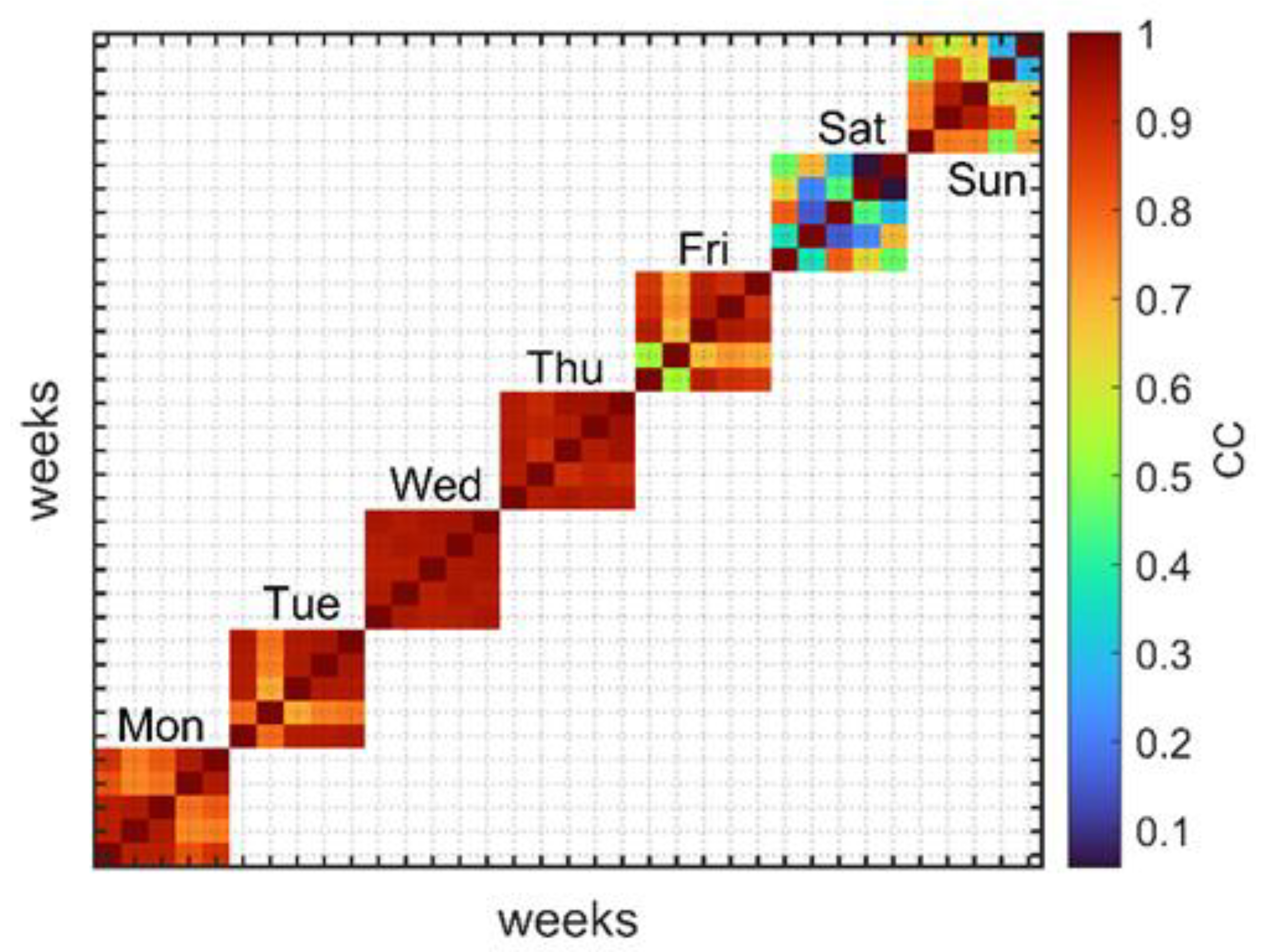
The relationships between the measured RF-EMF data on the same days in different weeks are presented in terms of correlation coefficients in Figure 9. It can be concluded from the figure that the RF-RMF levels measured on Wednesday and Thursday are highly correlated compared to the other days. The highest correlation between the days was calculated as 0.9543 on Thursday between the 4th and 5th weeks. The correlation values between Saturday and Sunday vary considerably compared to weekdays. This may be because there are specific activities on campus on certain weekends (e.g., exams, conferences).

Figure 9.
Daily cross correlation coefficients of RF-EMF levels for each week.
3.3. RF-EMF Prediction
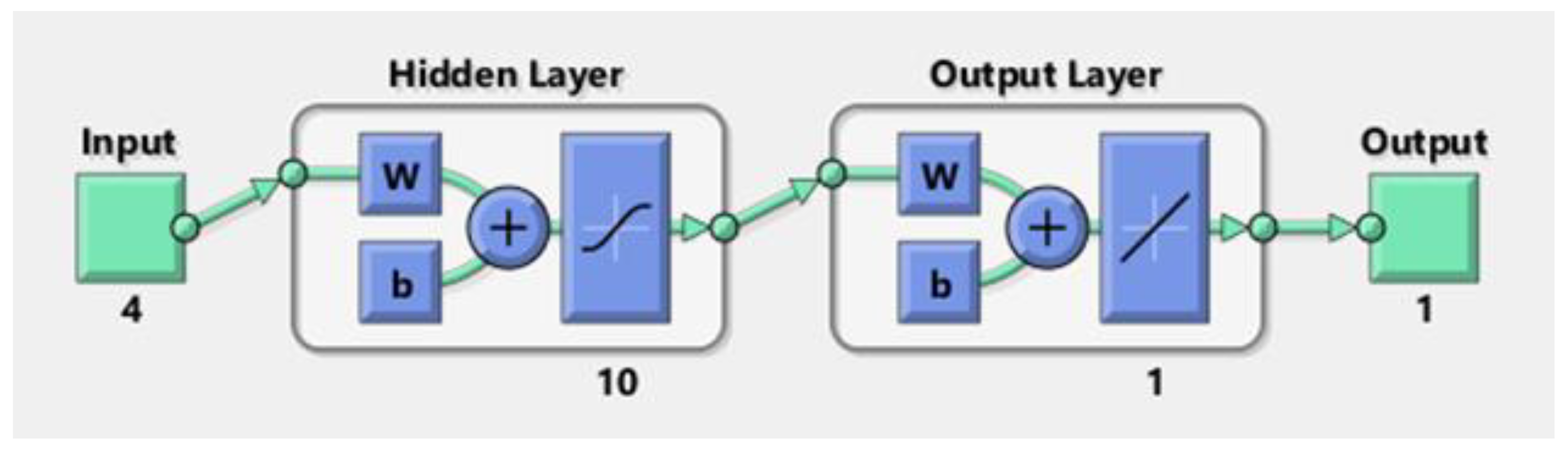
In order to determine the effects of weekly changes in RF-EMF levels within daily RF-EMF levels, an ANN model with ten sigmoid hidden neurons was created using the Neural Network Fitting tool in MATLAB. Figure 10 shows the structure diagram of the proposed ANN model.
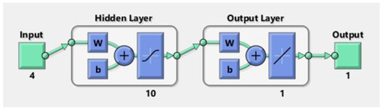
Figure 10.
Proposed artificial neural network model.
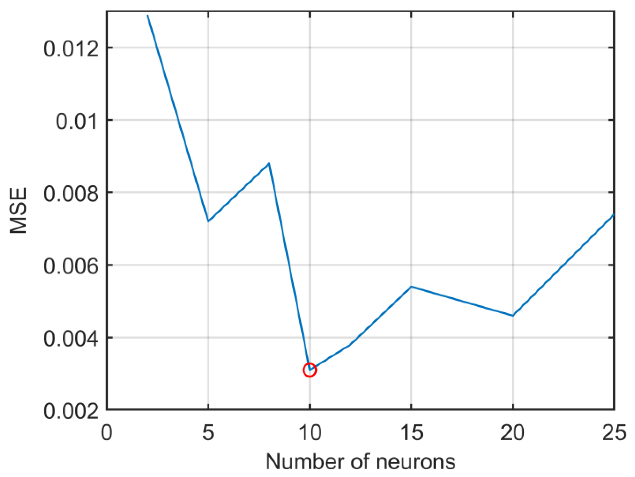
The optimal number of hidden neurons in this model was determined by randomly partitioning the input data and evaluating the test MSE for various numbers of neurons (max. 25 neurons) using the same partitioned data. The number of neurons that resulted in the minimum test MSE was chosen. The change in test MSE versus the number of hidden neurons used are presented in Figure 11.
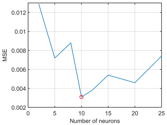
Figure 11.
The change in MSE versus number of neurons.
The post-processed RF-EMF data for the same days of the first four weeks were randomly partitioned into 70% training, 15% validation, and 15% testing. The first four week’s measurement data were used as input, while the fifth week’s data were used as target. The training stopped when either the number of epochs reached 1000 or the validation criterion was met. Because each training had different initial weights and biases, the network was trained fifty times with the LM and the BR algorithm, and the averaged results were given.
4. Results and Discussion
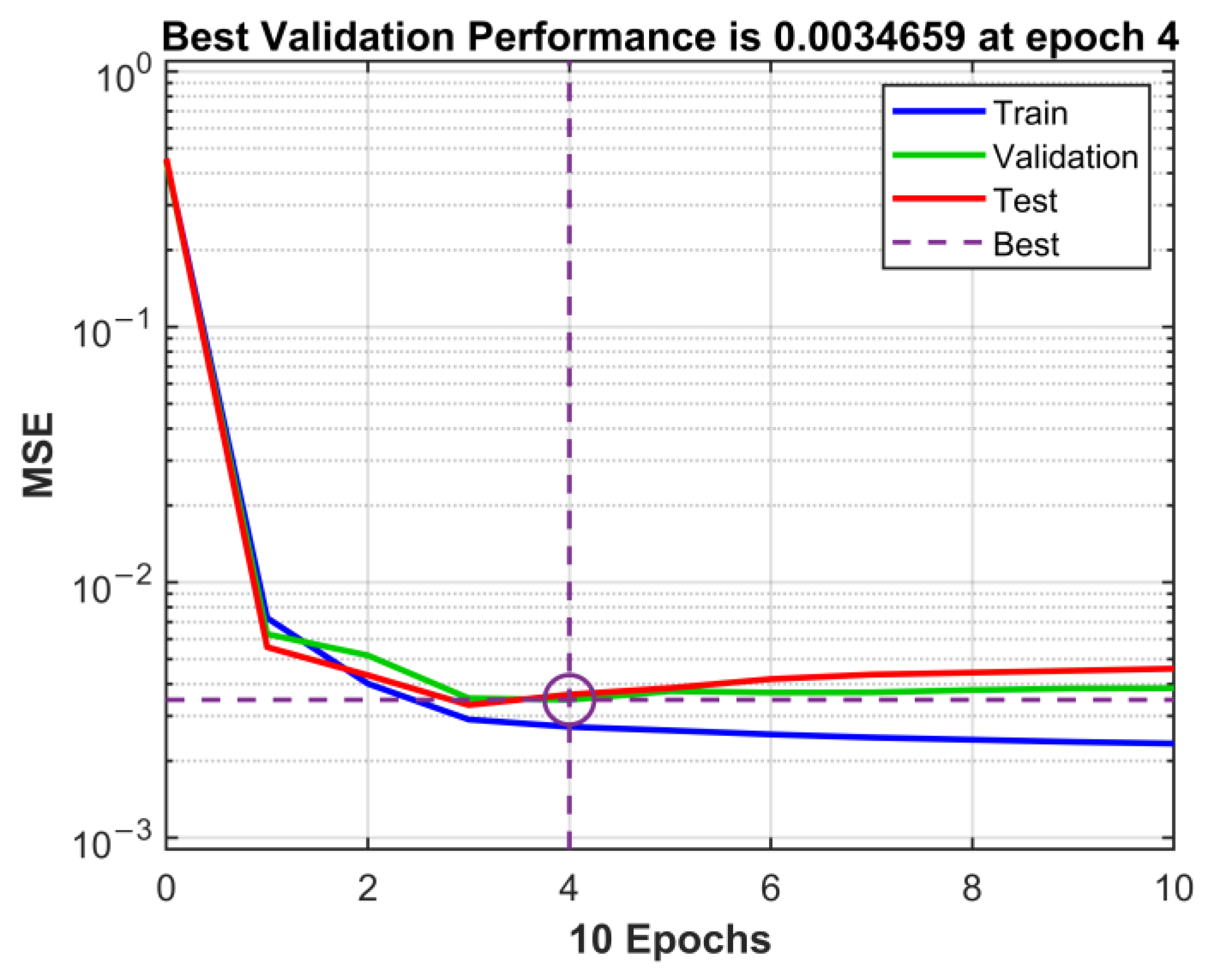
Regression analysis was performed for training data, testing data, validation data, and all data for fifty times, and the performances were averaged. MSEs and state transition performances were determined, and error histograms and regression plots were obtained. For the sake of brevity, only the results of the LM for Monday are given in the following figures. Figure 12 shows the MSE performance for training, validation, and test data as a function of epoch for one randomly selected run of the LM. As seen from the figure, the best validation performance was achieved at four epochs, with an MSE value of 3.47 × 10⁻³.
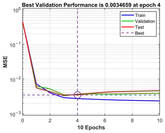
Figure 12.
MSE performance of the LM for Monday (for one randomly selected run).
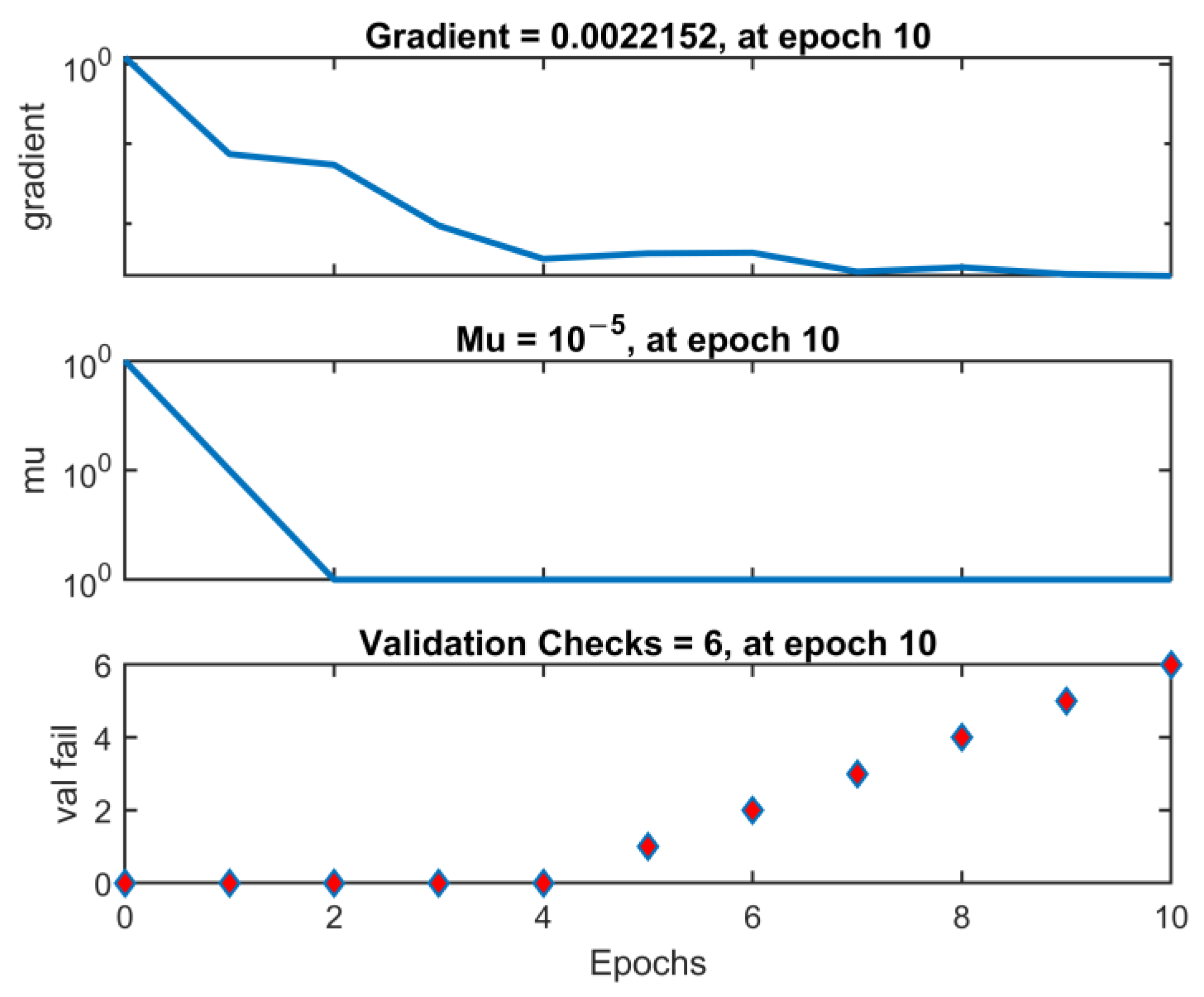
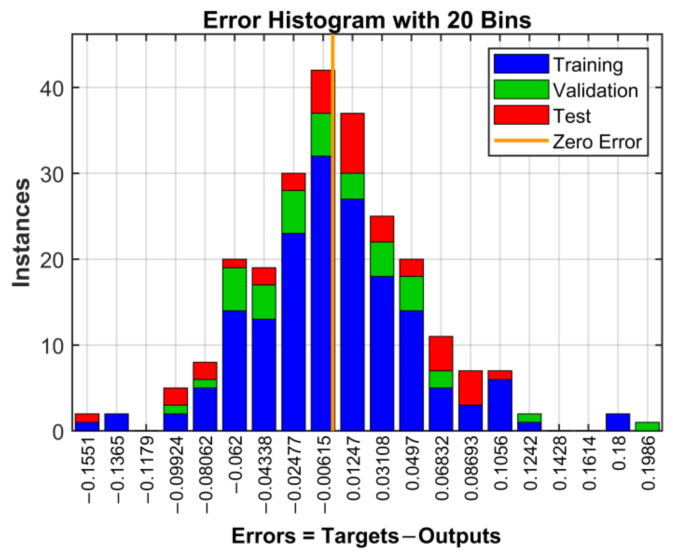
Figure 13 illustrates the training state values for one randomly selected run, in which the value of the gradient after ten epochs was 2.22 × 10⁻³ and mu was 1.00 × 10⁻⁵. The training process has been ended after six validation failures. The error histogram of one run with a reference zero error line is shown in Figure 14. Though there are some outliers; these data points are not largely different, and the error histogram roughly follows a normal distribution.
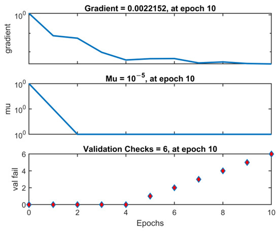
Figure 13.
Training state of the LM for Monday (for one randomly selected run).
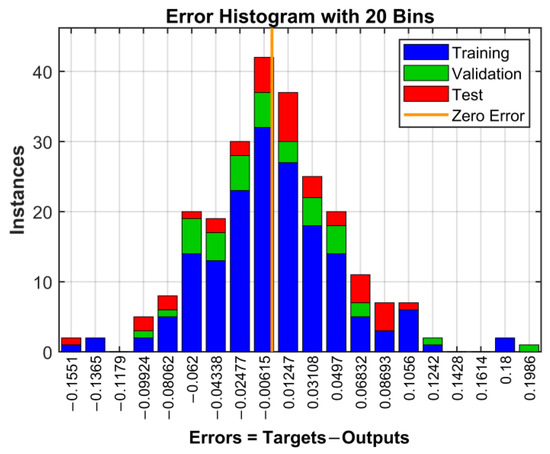
Figure 14.
Error histogram of the LM for Monday (for one randomly selected run).
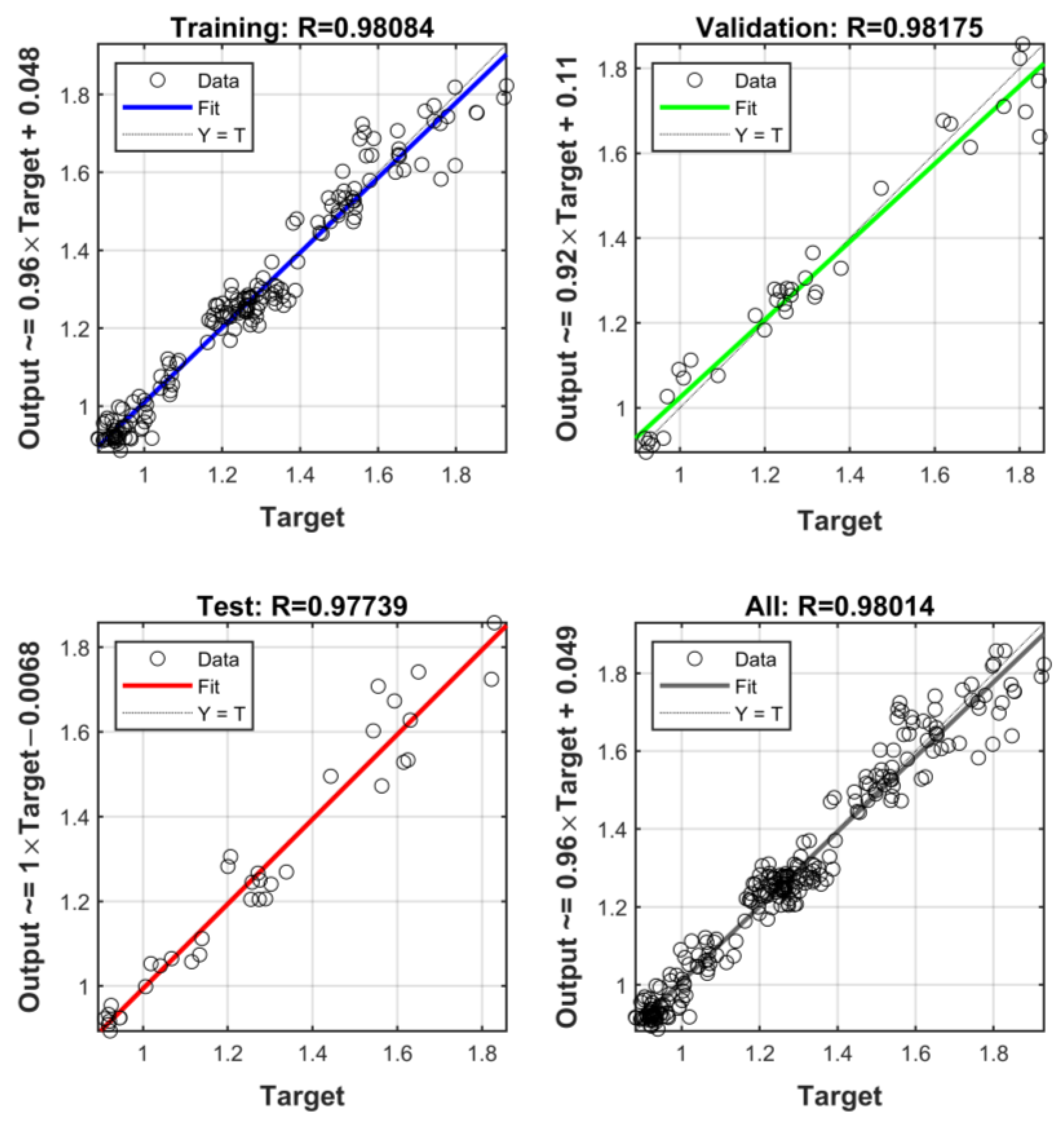
The regression plots of the average of fifty runs for training, validation, testing, and all data are given in Figure 15. It can be seen from the figures that the average regression coefficient, R, is 0.981 for training data, and the average R for validation, testing, and all data are 0.982, 0.977, and 0.980, respectively, which indicates a strong correlation and high performance.
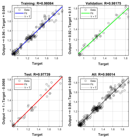
Figure 15.
Average regression performance of the LM for Monday.
In order to evaluate the overall performance of LM and BR, the average MSE values, epochs, and performances are tabulated in Table 3 and Table 4. Additionally, R values for LM and BR are listed in Table 5 and Table 6, respectively. As seen from Table 3 and Table 4, the performances of both methods are approximately 3 × 10⁻³. The MSE values for training, validation, and testing change between 2.58 × 10⁻³ to 4.08 × 10⁻³ for the LM method, while the values for training and testing for the BR method varies between 2.28 × 10⁻³ and 5.73 × 10⁻³. Although there is no noticeable difference between the MSE values of both methods, the LM-based method reaches a similar validation and training error with a smaller average number of epochs.
Table 3.
Performance evaluation of the LM.
Table 4.
Performance evaluation of the BR.
Table 5.
R values for the LM.
Table 6.
R values for the BR.
As can be seen from Table 5 and Table 6, the average correlation performance ranged from 0.826 to 0.982 for LM, while ranging between 0.854 to 0.982 for the BR method. The higher and closer the respective R values are to 1, the better the fit between the actual data and the predicted data; both methods have similar regression performances.
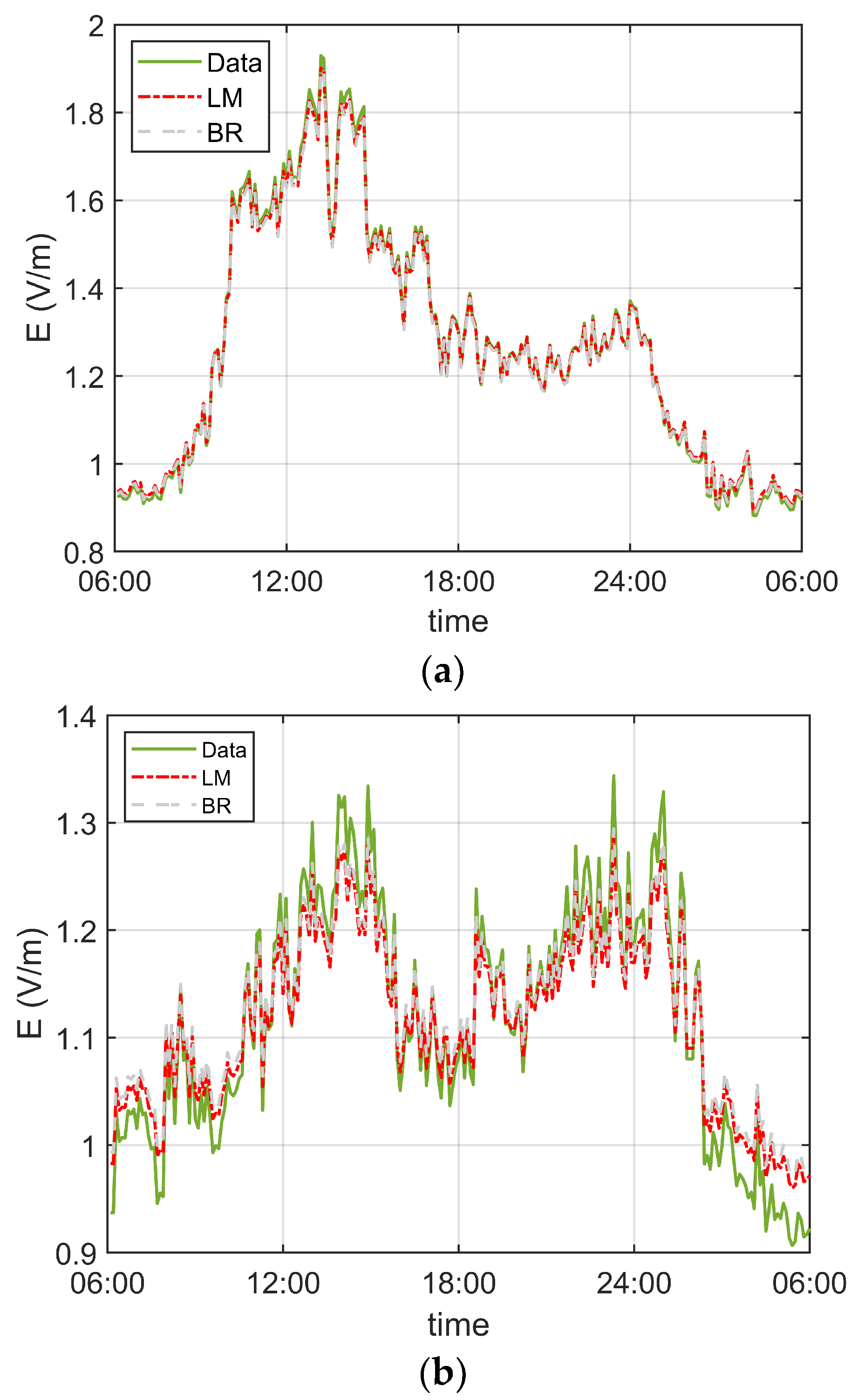
The highest average R values for all data were obtained for Monday for both methods, and the lowest was seen for Sunday. The fitting performances for these days are shown in Figure 16a,b, where the data represent target data for Monday and Sunday. As can be concluded from the figures, the reason for the best fitting of Monday’s data is the smooth fluctuations in the measured RF-EMF levels, whereas the deep fluctuations yield lower fitting performance for Sunday. When all of the data was analyzed, the developed LM and BR models showed similar fitting performances and could accurately predict the RF-EMF levels in the medium.
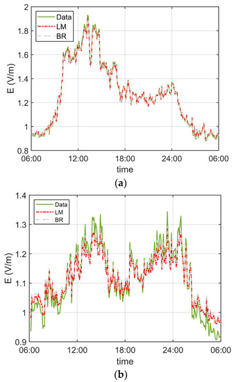
Figure 16.
Fit plot for (a) Monday, (b) Sunday.
The prediction performance of the LM model for Monday’s data was calculated, and the MSE was obtained as 1.86 × 10⁻⁵. The RMSE is 4.30 × 10⁻³, and the accuracy percentage is 99.6%. For the BR model, the corresponding values are 1.53 × 10⁻⁴, 12.3 × 10⁻³, and 98.8%, respectively. A similar assessment was performed on Sunday’s data, and the results were 7.25 × 10⁻⁴, 26.9 × 10⁻³, 93.8% for the LM, respectively, and 8.83 × 10⁻⁴, 29.7 × 10⁻³, and 93.2% for the BR model, respectively.
It can be concluded from the results that the proposed ANN models’ prediction accuracy is significantly better than similar works [17,25,31,32,33] in terms of the MSE, RMSE, and accuracy percentage. In [31], the MSE values ranged from 7.9 to 16.3, while [25] reported varying MSE values between 0.11 and 0.61 for the proposed model. The work of [32] reported an MSE of 1.5 × 10⁻³ for a fully connected ANN model, while the best MSE of 0.81 × 10⁻³ was achieved by a proposed hybrid connected model. Study [17] achieved an MSE of 2 × 10⁻³, and [33] obtained approximately 98% prediction accuracy for the proposed ANN model.
5. Conclusions
This study focuses on the prediction of RF-EMF levels at a university campus. First, band-selective measurements were performed to determine the contribution of 2G/3G/4G services to the total RF-EMF level. Contributions for each frequency band were extracted from these measurements, and it was proven that 99% of the total EMF in the environment originated from base stations. Then, the long-term RF-EMF measurements were conducted for 35 days in a location where the population density is high. The measurement results showed that weekly averaged RF-EMF levels varied between 1.1968 V/m and 1.3880 V/m, which are well below the ICTA’s limit. Additionally, the RF-RMF levels measured on Wednesday and Thursday showed a higher correlation compared to the other days. These measurement data were processed and utilized to create an ANN model with LM and BR learning algorithms to predict the RF-EMF levels. The average MSE performances of the proposed LM and BR models were evaluated, and there were no significant performance differences between the models. The regression performances of the models were also similar, and the best prediction performance was obtained for Monday with 99.6% accuracy, whereas Sunday’s performance was with an accuracy of 93.8%. The proposed models help to predict future RF-EMF levels accurately in the medium using existing measurement results.
Funding
This research received no external funding.
Institutional Review Board Statement
Not applicable.
Informed Consent Statement
Not applicable.
Data Availability Statement
The data that support the findings of this study are available from the corresponding author upon reasonable request.
Conflicts of Interest
The author declares no conflict of interest.
References
- Ramarakula, M. An efficient uplink power control algorithm for LTE-advanced relay networks to improve coverage area. Wireless Pers. Commun. 2020, 110, 1075–1087. [Google Scholar] [CrossRef]
- IARC. IARC Monographs on the Evaluation of Carcinogenic Risks to Humans. In Non-Ionization Radiation, Part 2: Radiofrequency Electromagnetic Fields; IARC Press: Lyon, France, 2013; Volume 102, 461p. [Google Scholar]
- Kaszuba-Zwoińska, J.; Gremba, J.; Gałdzińska-Calik, B.; Wójcik-Piotrowicz, K.; Thor, P.J. Electromagnetic field induced biological effects in humans. Przegl. Lek. 2015, 72, 636–641. [Google Scholar] [PubMed]
- Bilgici, B.; Gun, S.; Avci, B.; Akar, A.; Korunur Engiz, B. What is adverse effect of wireless local area network, using 2.45 GHz, on the reproductive system? Int. J. Radiat. Biol. 2018, 94, 1054–1061. [Google Scholar] [CrossRef] [PubMed]
- Alkis, M.E.; Bilgin, H.M.; Akpolat, V.; Dasdag, S.; Yegin, K.; Yavas, M.C.; Akdag, M.Z. Effect of 900-, 1800-, and 2100-MHz radiofrequency radiation on DNA and oxidative stress in brain. Electromagn. Biol. Med. 2019, 38, 32–47. [Google Scholar] [CrossRef]
- Cabré-Riera, A.; van Wel, L.; Liorni, I.; Thielens, A.; Birks, L.E.; Pierotti, L.; Joseph, W.; González-Safont, L.; Ibarluzea, J.; Ferrero, A.; et al. Association between estimated whole-brain radiofrequency electromagnetic fields dose and cognitive function in preadolescents and adolescents. Int. J. Hyg. Environ. Health 2021, 231, 113659. [Google Scholar] [CrossRef]
- Schuermann, D.; Mevissen, M. Manmade electromagnetic fields and oxidative stress—biological effects and consequences for health. Int. J. Mol. Sci. 2021, 22, 3772. [Google Scholar] [CrossRef]
- ICNIRP. Guidelines for limiting exposure to electromagnetic fields (100 kHz to 300 GHz). Health Phys. 2020, 118, 483–524. [Google Scholar] [CrossRef]
- ICTA. Ordinance Change on By-Law on Determination, Control and Inspection of the Limit Values of Electromagnetic Field Force from the Electronic Communication Devices According to International Standards; Law No.30394. 2018. Available online: https://www.resmigazete.gov.tr/eskiler/2018/04/20180417-2.htm/ (accessed on 21 September 2023).
- Kurnaz, C.; Engiz, B.K. Measurement and evaluation of electric field strength in Samsun city center. Int. J. Appl. Math. Electron. Comput. 2016, 4, 24–29. [Google Scholar] [CrossRef]
- Kurnaz, C.; Bozkurt, M.C. Measurement and evaluation of electromagnetic pollution levels in Ünye district of Ordu. J. N. Results Sci. 2016, 5, 149–158. [Google Scholar]
- Tang, C.; Yang, C.; Cai, R.S.; Ye, H.; Duan, L.; Zhang, Z.; Shi, Z.; Lin, K.; Song, J.; Huang, X.; et al. Analysis of the relationship between electromagnetic radiation characteristics and urban functions in highly populated urban areas. Sci. Total Environ. 2019, 654, 535–540. [Google Scholar] [CrossRef]
- Iyare, R.N.; Volskiy, V.; Vandenbosch, G.A.E. Study of the correlation between outdoor and indoor electromagnetic exposure near cellular base stations in Leuven, Belgium. Environ. Res. 2019, 168, 428–438. [Google Scholar] [CrossRef]
- Liu, J.; Wei, M.; Li, H.; Wang, X.; Wang, X.; Shi, S. Measurement and mapping of the electromagnetic radiation in the urban environment. Electromagn. Biol. Med. 2020, 39, 38–43. [Google Scholar] [CrossRef] [PubMed]
- Seyfi, L. Measurement of electromagnetic radiation with respect to the hours and days of a week at 100 kHz–3GHz frequency band in a Turkish dwelling. Measurement 2013, 46, 3002–3009. [Google Scholar] [CrossRef]
- Engiz, B.K.; Kurnaz, C. Long-term electromagnetic field measurement and assessment for a shopping mall. Radiat. Prot. Dosimetry 2017, 175, 321–329. [Google Scholar] [CrossRef] [PubMed]
- Karadag, T.; Yüceer, M.; Abbasov, T. A large-scale measurement, analysis and modelling of electromagnetic radiation levels in the vicinity of GSM/UMTS base stations in an urban area. Radiat. Prot. Dosim. 2016, 168, 134–147. [Google Scholar] [CrossRef] [PubMed]
- Aerts, S.; Wiart, J.; Martens, L.; Joseph, W. Assessment of long-term spatio-temporal radiofrequency electromagnetic field exposure. Environ. Res. 2018, 161, 136–143. [Google Scholar] [CrossRef] [PubMed]
- Kurnaz, C.; Mutlu, M. Comprehensive radiofrequency electromagnetic field measurements and assessments: A city center example. Environ. Monit. Assess. 2020, 192, 334. [Google Scholar] [CrossRef]
- Kurnaz, C.; Mutlu, M. Monitoring and modelling of long-term radiofrequency electromagnetic field levels. J. Fac. Eng. Archit. Gazi Univ. 2021, 36, 669–683. [Google Scholar] [CrossRef]
- Rivera González, M.X.; Félix González, N.; López, I.; Ochoa Zambrano, J.S.; Miranda Martínez, A.; Maestú Unturbe, C. Compact exposimeter device for the characterization and recording of electromagnetic fields from 78 MHz to 6 GHz with several narrow bands (300 kHz). Sensors 2021, 21, 7395. [Google Scholar] [CrossRef]
- Neskovic, A.; Neskovic, N.; Paunovic, D. Indoor electric field level prediction model based on the artificial neural networks. IEEE Commun. Lett. 2000, 4, 190–192. [Google Scholar] [CrossRef]
- Neskovic, A.; Neskovic, N.; Paunovic, D. Macrocell electric field strength prediction model based upon artificial neural networks. IEEE J. Sel. Areas Commun. 2002, 20, 1170–1177. [Google Scholar] [CrossRef]
- Neskovic, A.; Neskovic, N. Microcell electric field strength prediction model based upon artificial neural networks. AEU- Int. J. Electron. Commun. 2010, 64, 733–738. [Google Scholar] [CrossRef]
- Isabona, J. Wavelet generalized regression neural network approach for robust field strength prediction. Wirel. Pers. Commun. 2020, 114, 3635–3653. [Google Scholar] [CrossRef]
- Fraiha Lopes, R.L.; Fraiha, S.G.; Lima, V.D.; Gomes, H.S.; Cavalcante, G.P. Hybrid ARIMA and neural network modelling applied to telecommunications in urban environments in the Amazon region. Int. J. Antennas Propag. 2020, 2020, 2671746. [Google Scholar] [CrossRef]
- Alihodzic, A.; Mujezinovic, A.; Turajlic, E. Electric and magnetic field estimation under overhead transmission lines using artificial neural networks. IEEE Access 2021, 9, 105876–105891. [Google Scholar] [CrossRef]
- Sakacı, F.H.; Cerezci, O. Prediction of magnetic pollution with artificial neural network in living areas. J. Electr. Eng. Technol. 2021, 16, 2701–2708. [Google Scholar] [CrossRef]
- Li, R.; Yue, Y.; Song, X.; Ji, S. Measurement and prediction of indoor wideband electric field radiation. IEEE Trans. Instrum. Meas. 2021, 70, 6504612. [Google Scholar] [CrossRef]
- Aerts, S.; Vermeeren, G.; Van den Bossche, M.; Aminzadeh, R.; Verloock, L.; Thielens, A.; Leroux, P.; Bergs, J.; Braem, B.; Philippron, A.; et al. Lessons learned from a distributed RF-EMF sensor network. Sensors 2022, 22, 1715. [Google Scholar] [CrossRef]
- Wang, S.; Wiart, J. Sensor-aided EMF exposure assessments in an urban environment using artificial neural networks. Int. J. Environ. Res. Public. Health 2020, 17, 3052. [Google Scholar] [CrossRef]
- Wang, S.; Mazloum, T.; Wiart, J. Prediction of RF-EMF exposure by outdoor drive test measurements. Telecom 2022, 3, 396–406. [Google Scholar] [CrossRef]
- Karpat, E.; Bakcan, M.R. Measurement and prediction of electromagnetic radiation exposure level in a university campus. Teh. Vjesn. 2022, 29, 449–455. [Google Scholar] [CrossRef]
- Hagan, M.T.; Menhaj, M.B. Training feedforward networks with the Marquardt algorithm. IEEE Trans. Neural Netw. 1994, 5, 989–993. [Google Scholar] [CrossRef] [PubMed]
- Jaiswal, P.; Gupta, N.K.; Ambikapathy, A. Comparative Study of Various Training Algorithms of Artificial Neural Network. In Proceedings of the International Conference on Advances in Computing, Communication Control and Networking (ICACCCN), Greater Noida, India, 12–13 October 2018; pp. 1097–1101. [Google Scholar] [CrossRef]
- SRM-3006, Band Selective EMF Meter. Available online: https://www.narda-sts.com/en/selective-emf/srm-3006-field-strength-analyzer/ (accessed on 16 September 2023).
- Kurnaz, C.; Engiz, B.K.; Kose, U. An empirical study: The impact of the number of users on electric field strength of wireless communications. Radiat. Prot. Dosimetry 2018, 182, 494–501. [Google Scholar] [CrossRef] [PubMed]


Disclaimer/Publisher’s Note: The statements, opinions and data contained in all publications are solely those of the individual author(s) and contributor(s) and not of MDPI and/or the editor(s). MDPI and/or the editor(s) disclaim responsibility for any injury to people or property resulting from any ideas, methods, instructions or products referred to in the content. |
© 2023 by the author. Licensee MDPI, Basel, Switzerland. This article is an open access article distributed under the terms and conditions of the Creative Commons Attribution (CC BY) license (https://creativecommons.org/licenses/by/4.0/).