Abstract
Deep neural networks (DNNs) have gained prominence in addressing regression problems, offering versatile architectural designs that cater to various applications. In the field of earthquake engineering, seismic response prediction is a critical area of study. Simplified models such as single-degree-of-freedom (SDOF) and multi-degree-of-freedom (MDOF) systems have traditionally provided valuable insights into structural behavior, known for their computational efficiency facilitating faster simulations. However, these models have notable limitations in capturing the nuanced nonlinear behavior of structures and the spatial variability of ground motions. This study focuses on leveraging ambient vibration (AV) measurements of buildings, combined with earthquake (EQ) time-history data, to create a predictive model using a neural network (NN) in image format. The primary objective is to predict a specific building’s earthquake response accurately. The training dataset consists of 1197 MDOF 2D shear models, generating a total of 32,319 training samples. To evaluate the performance of the proposed model, termed MLPER (machine learning-based prediction of building structures’ earthquake response), several metrics are employed. These include the mean absolute percentage error (MAPE) and the mean deviation angle (MDA) for comparisons in the time domain. Additionally, we assess magnitude-squared coherence values and phase differences () for comparisons in the frequency domain. This study underscores the potential of the MLPER as a reliable tool for predicting building earthquake responses, addressing the limitations of simplified models. By integrating AV measurements and EQ time-history data into a neural network framework, the MLPER offers a promising avenue for enhancing our understanding of structural behavior during seismic events, ultimately contributing to improved earthquake resilience in building design and engineering.
1. Introduction
Deep neural networks (DNNs) have gained significant popularity in addressing regression problems, and numerous architectural designs have become prevalent. One such architecture is the multi-layer perceptron (MLP), which has been widely employed in various regression problems [1]. The developers of the MLP are acknowledged for introducing the backpropagation algorithm, a key method for training neural networks [2]. Another notable architecture is the convolutional neural network (CNN) introduced by LeCun et al. [3,4,5,6]. CNNs are extensively utilized in image and signal processing tasks and have also found application in regression tasks. Recurrent neural networks (RNNs), initially introduced by John Hopfield in the early 1980s [7], gained widespread adoption with the advent of the long short-term memory (LSTM) architecture developed by Hochreiter and Schmidhuber in 1997 [8]. LSTMs have proven highly effective in capturing long-term dependencies in sequential data. During the mid-2000s, Restricted Boltzmann Machines (RBMs) and deep belief networks (DBNs) played a pivotal role in the advancement of deep learning techniques, particularly in unsupervised learning and feature learning [9]. Between 2000 and 2017, advancements such as dropout, batch normalization, convolutional LSTMs, and residual connections further enhanced the performance of existing architectures for regression tasks. Transformers, a more recent architectural design, have exhibited remarkable success in natural language processing tasks and exhibit potential for regression tasks [10]. Furthermore, it is crucial to emphasize the effectiveness of DNNs in addressing two particularly challenging concepts. The first concept involves using available photographs to assess seismic vulnerability, which can be appropriately processed to provide input data for empirical vulnerability algorithms [11]. The second concept revolves around the automated detection of defects in existing reinforced concrete (RC) bridges, necessitating the application of diverse deep learning (DL) methodologies and techniques to interpret the resulting predictions [12].
Meanwhile, seismic response prediction is an important aspect of earthquake engineering, and simplified models such as the SDOF and MDOF systems can provide valuable insights into the behavior of structures, being advantageous due to their processing efficiency, which allows for faster and more manageable computational simulations. However, these simplified models have limitations, particularly in accurately capturing the nonlinear behavior of structures and the spatial variability of ground motions, which is something we shall bear in mind. Software tools and methodologies such as Hazus-MH 2.1 in the United States [12], pre-quake rapid visual inspection (RVI) in Greece [13], and the FEMA P-58 methodology [14] have been developed to enable fast-track inspections and risk estimations for large building stock. Open-source software frameworks such as OpenSees, version 3.5.0 [15] and OpenQuake version 3.17.1 [16] have also been developed, which provide a platform for researchers and engineers to develop and apply advanced techniques for seismic response prediction, including machine learning and hybrid simulation. For example, OpenQuake has been used for probabilistic seismic hazard assessments and loss estimations [17]. While these tools have their own limitations, ongoing research is focused on improving their accuracy and applicability through advanced techniques and open-source software. Additionally, advancements in big data and structural health monitoring have created new opportunities for seismic response prediction methods. Structural health monitoring systems, such as accelerographs, provide real-time data on the behavior of structures during seismic events, enabling a detailed understanding of their response. This data, along with geological and seismic activity data, can be used to build large datasets for machine learning and other advanced techniques [18,19]. Various machine learning-based approaches have been made such as predicting the seismic damage to building structures considering soil–structure interaction effects [20], their seismic performance levels [21] or even damage identification [22]. Other studies have dealt with the various dynamic quantities of building structures such as acceleration, and the displacement response quantities trying to manipulate them [23].
This study primarily focuses on utilizing ambient vibration (AV) measurements from a building in conjunction with earthquake (EQ) time histories, which are processed through a neural network (NN) in image format to predict the building’s specific earthquake response. The training phase involved the development of 1197 multi-degree-of-freedom (MDOF) 2D shear models, resulting in the creation of a total of 32,319 samples. To assess the NN’s performance, various metrics were employed, including the MAPE (mean absolute percentage error), MDA (mean difference amplitude) for time-history comparisons, and magnitude-squared coherence values and phase difference () for frequency domain comparisons. This proposed model is named MLPER, which stands for machine learning-based prediction of building structures’ earthquake response.
The remainder of this study is structured as follows: Section 1 presents the structural parameters employed in dataset creation, outlines the assumptions made regarding the MDOF 2D shear models, and provides the list of earthquake recordings used, along with their characteristics. Section 2 offers an overview of the available deep neural network options, highlighting their suitability for addressing the specific problem at hand. It delves into the reasoning behind the rejection of some options and the preference for others in the context of the regression task. It also discusses the underlying principles and the chosen structural parameters of the model. Section 3 examines the format of the training data and discusses decisions made regarding their utilization in the neural network training process. Section 4 provides a detailed description of the MLPER architecture, while Section 5 presents the results using various metrics to assess performance. Section 6 concludes the study, offering remarks on performance and suggesting avenues for future work within the presented network framework.
2. Structural Models Used for Generating the Calibration Data
In this study, the objective is to develop a neural network-based model capable of predicting the response, specifically the acceleration time history, of the top floor translational degree of freedom of a multi-degree-of-freedom (MDOF) building system when subjected to an earthquake event, without relying on any finite element analysis. The underlying motivation behind this endeavor is to eventually contribute, with a refined neural network model, to a rapid estimation of a structure’s response, accounting for its nonlinear behavior and the characteristics of the ground, at least in bilinear terms, by utilizing field measurements. More specifically, the proposed model will combine ambient response timeframes of 60 s with earthquake timeframes. For each set of inputs, consisting of the ambient top floor response and the earthquake data, the model will produce the response of the specific MDOF system to the specific seismic event.
The data and measurements employed in this study were obtained through a rigorous process involving numerical generation and computational derivation, utilizing the Newmark numerical integration method. This approach was selected to encompass a wide range of MDOF models, ensuring the inclusion of all possible parameter combinations. A comprehensive set of 1197 models was specifically utilized for the purpose of this investigation, ensuring a robust and extensive analysis.
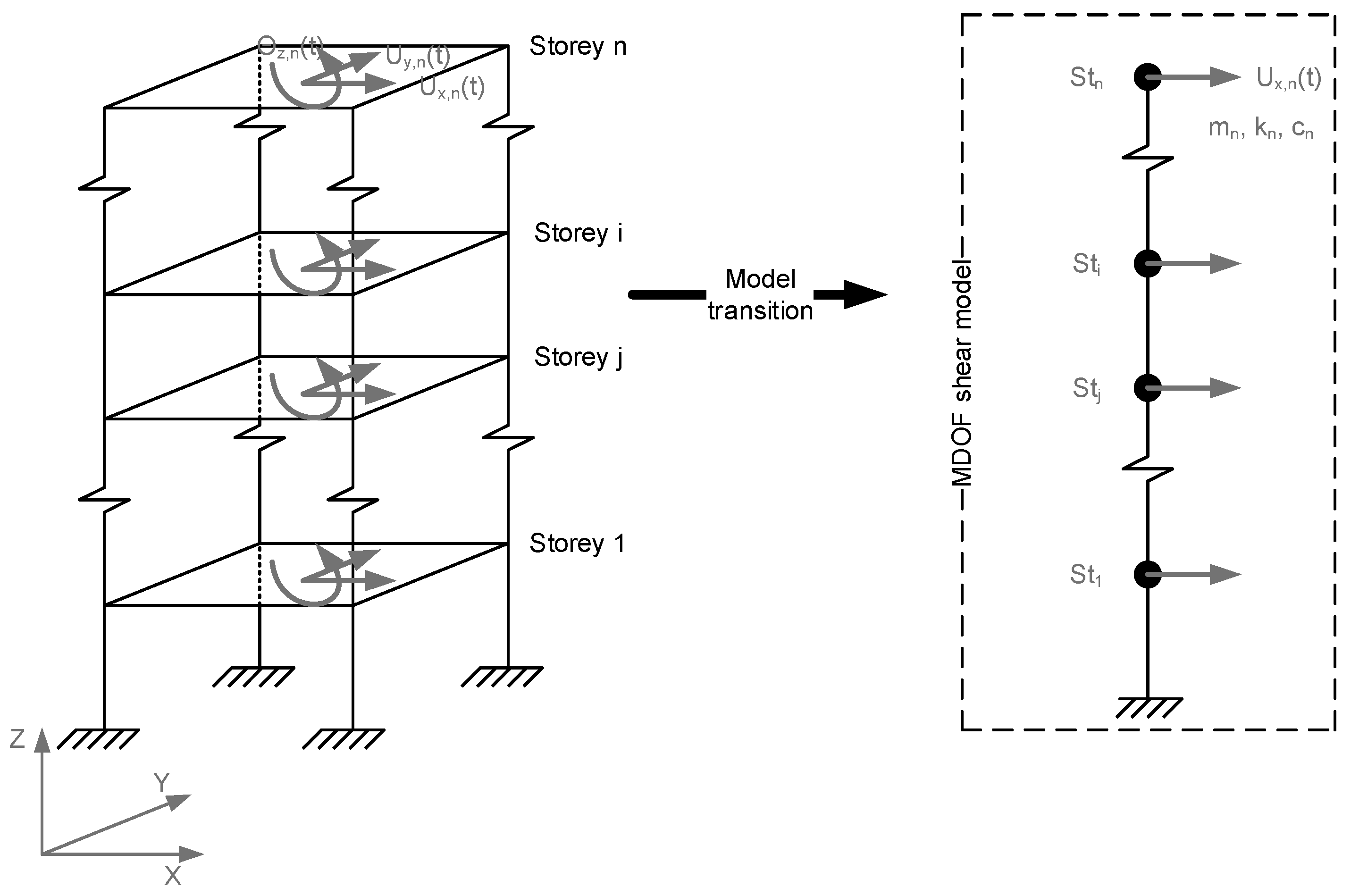
The assumptions used to construct these models were based on a building model that can be seen in Figure 1. This reference building model was mainly used for the estimation of the mass baseline per floor. The stiffness matrix is also seen in Table 1. However, the stiffness value was derived after setting the target frequency and target mass. This model was developed using the ADINA v. 9.1.1 analysis software [24]. The number of assumptions and parameters used are shown in Table 1.

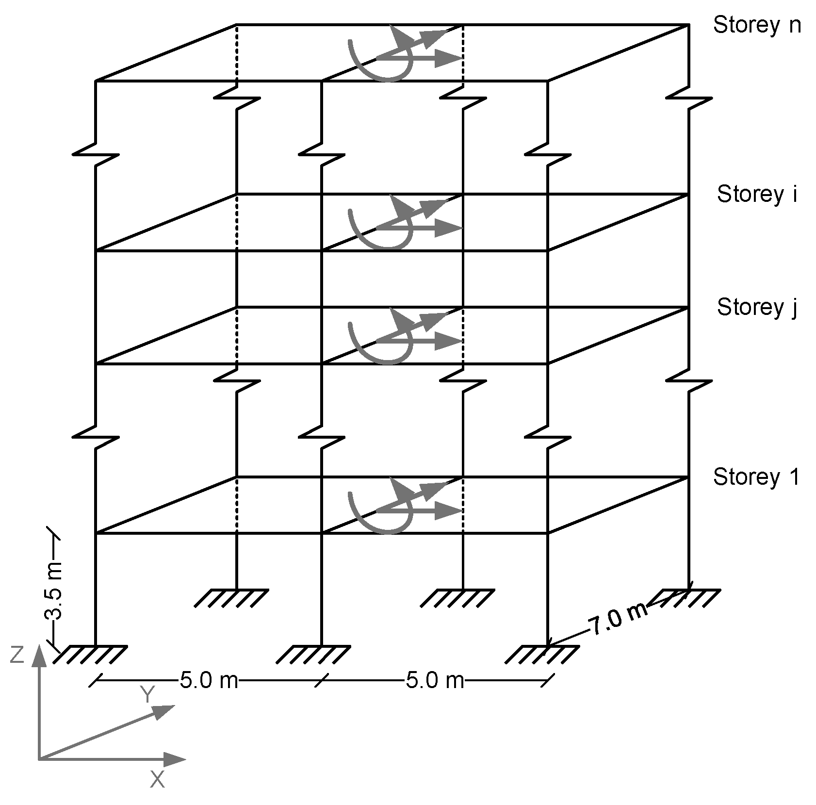
Figure 1.
The assumptions table is referring to the typical building model, (the grey arrows denote the three DOFs per storey of the fully fixed frame structure).
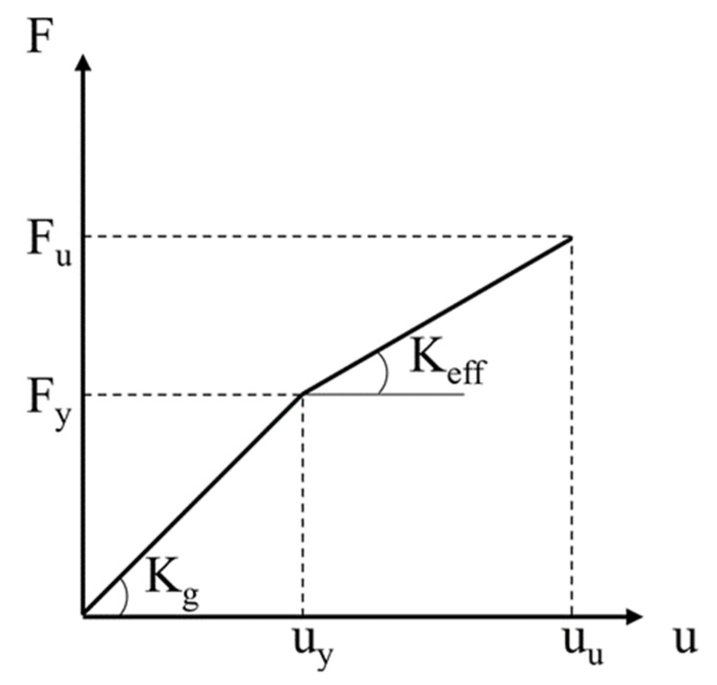
To capture some level of the nonlinearity of material or/and level of damage, a bilinear capacity curve was constructed, which applied to all structural members of each MDOF model (Figure 2). The general layout of the curve is illustrated in Figure 3 (bilinear capacity curve of all structural members). Each numerically produced ambient acceleration response signal is the sum of the ambient excitation itself with the response of the corresponding MDOF model at the last degree of freedom (top of the building). The case study did not incorporate the soil–structure interaction (SSI). Nevertheless, it can be readily incorporated by utilizing a system of horizontal and vertical springs within fictitious elements, which simulate the diverse bedrock layers and their influence on the structure [25].

Figure 2.
The MDOF 2D shear model.

Figure 3.
Bilinear capacity curve of all structural members, where yielding and ultimate states are denoted.

Table 1.
Models’ generation parameters.
Table 1.
Models’ generation parameters.
| Geometry | |||
| Plan | 10.00 × 7.00 (m2) | ||
| Stories | 1 to 7 | ||
| Story height | 3.50 (m) | ||
| Slab thickness | 0.25 (m) | ||
| Columns | 0.50 × 0.50 (m2) | ||
| Beams | 0.40 × 0.70 (m2) | ||
| Loads | |||
| Dead | 806.75 (kN) | ||
| Live | 806.75 (kN) | ||
| Safety factor | 1 1 | ||
| Dynamic Characteristics | |||
| Mass (per story) | 110.78 (tons) | ||
| Damping ratio ζ | 5% | ||
| Eigenfrequency | 1 to 10 Hz with step of 0.5 | ||
| Material | |||
| Reinforced concrete | |||
| Bilinear material | Figure 3 | ||
| Yield point (uy) | 0.0105 (m) 2 | ||
| Post yield stiffness (Keff) | 50% of geometric one (Kg) 3 | ||
| Shear building model | K matrix for N = 3 (stories) | ||
| k1 + k2 | −k2 | 0 | |
| −k2 | k2 + k3 | −k3 | |
| 0 | −k3 | k3 | |
1 Assessment of existing condition—real loads. 2 0.003 drift × 3.50 m = 0.0105 m (Hazus C3L—LowCode). More details can be found in Hazus ® {MH 2.1 Technical Manual (see Paragraph 5.2.1 of [26]). 3 EC8–1 (), after the first yield, loading-unloading is implemented using even for the cases where .
The signals in this study have a sampling rate of 100 Hz, and their duration is consistently 60 s. It is important to note that these signals are intentionally generated without any electronic noise. This is because it is assumed that the measurements will either be obtained using low noise accelerographs or processed using some form of neural network for denoising the signal. Each building model in the dataset comprises 1 to 7 floors, with a mass ranging from 80% to 120% of the typical values mentioned in Table 1 and with an eigenfrequency ranging between 1 and 10 Hz with a step of 0.5 Hz. Therefore, 1197 models of MDOF models were derived. For each of these models, three timeframes of ambient response were selected, leading to the generation of 3591 artificial ambient responses.
In terms of earthquake signals, nine acceleration time histories were carefully chosen to accompany the ambient response signals. These earthquakes are classified into categories of low, medium, and high amplitudes (refer to Table 2 and Figure 4). For each earthquake scenario, model responses were generated, resulting in a total of 10,773 earthquake responses. These earthquake responses will be combined with the corresponding 3591 ambient responses, bringing the total number of cases in the created dataset to 32,319. Again, it is important to mention that all signals in the dataset are sampled at 100 Hz and have a duration of 60 s.
Table 2.
List of seismic records used for developing the training and validation sets.
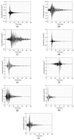
Figure 4.
Earthquakes adopted for generating the training–validation sets; starting from ID 1 to ID 9 (a–i).
The split to training and validation datasets was made on the model’s level. Meaning that from the 1197 models, ~75% of them are used for training (training set), while the other ~25% (299 models/~8100 samples) are used as the validation sample (validation set). Therefore, the network learns to predict the response on unforeseen models for the 9 “known” EQs.
3. Neural Network Architecture Options
Neural networks are computational models that draw inspiration from the structure and functioning of the human brain. These models comprise interconnected layers of artificial neurons (known also as nodes), which process information by emulating the communication between biological neurons. As data traverse the network, each neuron processes and transforms the input, progressively constructing a hierarchy of increasingly intricate features. During training, the network fine-tunes its weights and biases through a process known as learning (by means of an algorithmic procedure like backpropagation), which minimizes the discrepancy between its predictions and the actual output. Through iterative search optimization, neural networks acquire the ability to discern intricate patterns, generalize from the training data, and effectively tackle complex tasks like image recognition, natural language processing, and decision making.
The problem at hand can be characterized as a deterministic regression task. However, due to the specific nature of the system inputs, employing a popular generative adversarial network (GAN) architecture was deemed unsuitable. GANs generate outputs that are non-deterministic, meaning that the same input can yield different outputs each time the model is used. This behavior arises from the stochastic processes utilized by GANs, such as incorporating random noise during sample generation. Furthermore, the output of GANs is highly reliant on factors like training data, hyperparameter selection, and the training process itself. While GANs can produce impressive and realistic results, they do not offer a unique and definitive solution to a given problem. Even when considering the subclass of GANs known as conditional generative adversarial networks (CGANs), which can be trained to generate samples conditioned on specific input information, the results were still not deterministic. As a result, an alternative approach was pursued using recurrent neural networks (RNNs), specifically the long short-term memory (LSTM) architecture. LSTMs can mitigate the vanishing gradient problem often encountered in traditional RNNs. Another option considered for the regression task was to employ convolutional neural networks (CNNs). However, considering the substantial size of the dataset (multiple gigabytes), the limitations of the LSTM in comparison to CNNs were taken into careful consideration.
- Computationally expensive: LSTMs are computationally expensive compared to CNNs, as they require a more complex architecture and involve more computations. This can make them more challenging to train and deploy, especially in real-time applications.
- Limited parallelization: LSTMs are less parallelizable compared to CNNs, as the computations in LSTMs are sequential and depend on the output of previous time steps. This can limit their scalability and make them less suitable for high-performance computing applications.
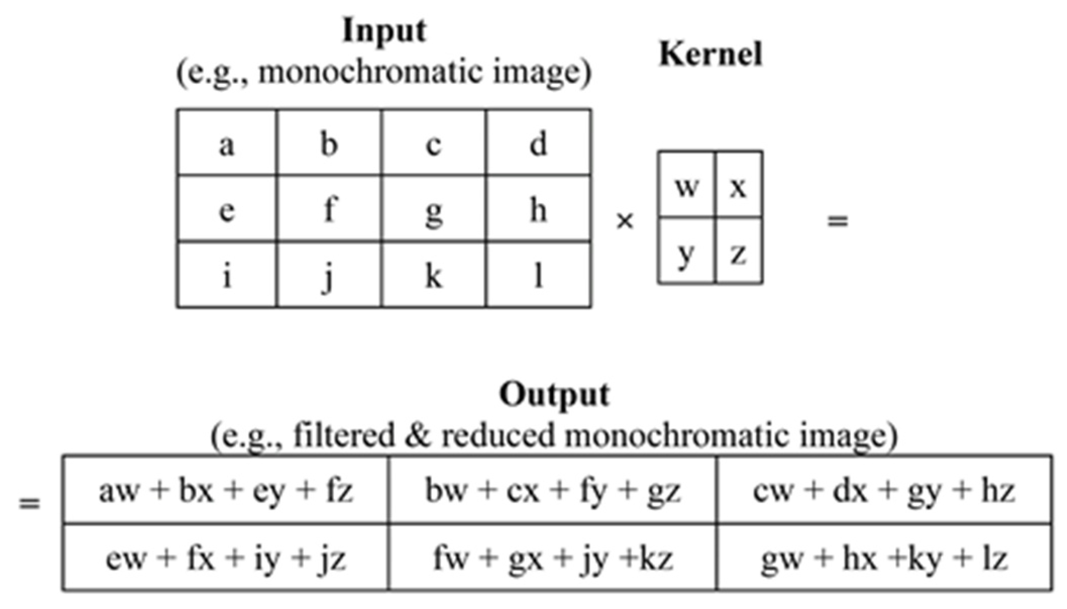
In the context of the proposed neural network architecture, CNN layers were selected as a fundamental component. Convolutional networks (e.g., LeCun et al. [3,4,5,6]), often referred to as convolutional neural networks (CNNs), were chosen due to their specialized nature in handling data with grid-like structures. Such grid-like data examples encompass time-series data, which can be conceptualized as a 1D grid with regularly spaced time interval samples, as well as image data, which can be visualized as a 2D grid composed of pixels. Convolutional networks have exhibited remarkable success in practical applications, and the term “convolutional neural network” reflects their utilization of a mathematical operation known as convolution.
where x(t) is the raw signal measurement at time t, w(a) is a weighted average that gives more weight to recent measurements, a denotes the age of a measurement, and s(t) is the smoothed estimate of the x(t) measurement. Convolution is also denoted as follows:
In the terminology of convolutional networks, the initial parameter (referred to as function x) of the convolution operation is commonly denoted as the input, while the second parameter (referred to as function w) is known as the kernel. The resulting outcome is often termed the feature map (as illustrated in Figure 5). In our scenario, as well as in numerous other instances, the convolution operation is two-dimensional, and time is considered discrete. Consequently, its mathematical representation, known as convolution without flipping and equivalent to cross-correlation, can be expressed as follows:
where I is a two-dimensional array of data (e.g., an image) and K is a two-dimensional kernel; both I and K have discrete values.

Figure 5.
A 2D CNN channel.
4. Training Data Format
In coherence to use CNNs as the main form of our NN, the time series had to be converted into images. However, using images of time series in the time domain would be a bad decision, as the range of values in our dataset is large, characterized also by large outliers (maximum and minimum values) in comparison with the mean value of the time histories being around zero. This large range in scale can be seen in Figure 4, between (a) and (i). Moreover, the variation in values is also present between the different categories of the time series (Ambient Response, EQ excitation, Response under EQ). Specifically, the amplitude of time series used by the NN model varies as follows:
- Ambient Response: [−7.380213 × 10⁻⁵, 7.189604 × 10⁻⁵] (g)
- EQ excitation: [−3.54141, 5.57502] (m/sec2)
- Response under EQ: [−19.02244, 20.79666] (m/sec2)
Consequently, all time histories undertook a transformation from the time domain to the frequency domain. To achieve this, spectrograms representing both amplitude and phase information were derived for each signal in the time domain. As a result, two images were generated for each signal type, shifting the problem from a two-image input—one-image output to a two-set of two-image input—one-set of two-image output scenario (illustrated in Figure 6). The parameters used for the short-time Fourier Transform across the entire dataset were as follows: (a) 400 discrete Fourier transform (DFT) points, (b) a sampling rate of 100Hz, (c) a 6-sample overlapping window applied between adjacent segments, and (d) an 8-point symmetric Hann window used for segmenting the signal and applying windowing.
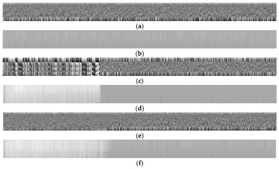
Figure 6.
A sample of input/output set of images for training, with (a) Ambient response phase (input), (b) Ambient response magnitude (input), (c) EQ excitation phase (input), (d) EQ excitation magnitude (input), (e) EQ response phase (output), and (f) EQ response magnitude (output).
Subsequently, the maximum and minimum values across the entire dataset were identified and employed to normalize all input and output categories uniformly. The magnitude spectrograms are presented in decibels (dB), ranging from −380 to +40 dB on a black-to-white color scale, while the phase spectrograms are represented in degrees, spanning from −π to +π degrees also on a black-to-white color scale.
The training and validation datasets consist of images with dimensions 2997 × 201 pixels, saved in .png format. These images are grayscale, meaning that each pixel is represented by a single integer within the range of [0, 255]. To optimize storage while preserving the necessary resolution, an 8-bit depth was selected. An 8-bit image offers a dynamic range of 48.13 dB, distinct from the time series data discussed later in the “Numerical investigation—results” section. TensorFlow neural network models typically employ 32-bit variables, occasionally dipping to 16-bit variables in mixed precision mode. For our experiments, we opted for the default 32-bit precision to ensure stability. Due to the dataset’s size, direct RAM loading is unfeasible. Consequently, we converted the images into TFRecords, a binary file format designed for efficient storage and processing within TensorFlow. TFRecords serialize data, transforming them into a sequence of bytes that can be effortlessly transmitted over networks or stored on disks. This format proves invaluable when handling substantial datasets, enabling efficient data streaming, shuffling, and random access. TFRecords accommodate various data types, including images, audio, text, and numerical data. They find widespread applications in TensorFlow for data preprocessing, augmentation, and input pipeline optimization. In total, the training dataset occupies approximately 342 GB, while the validation dataset consumes around 114 GB. To prepare the data for neural network input, standard scaling procedures are performed. This involves normalizing every pixel value to fall within the [0, 1] range by dividing by 255.
5. The MLPER Architecture
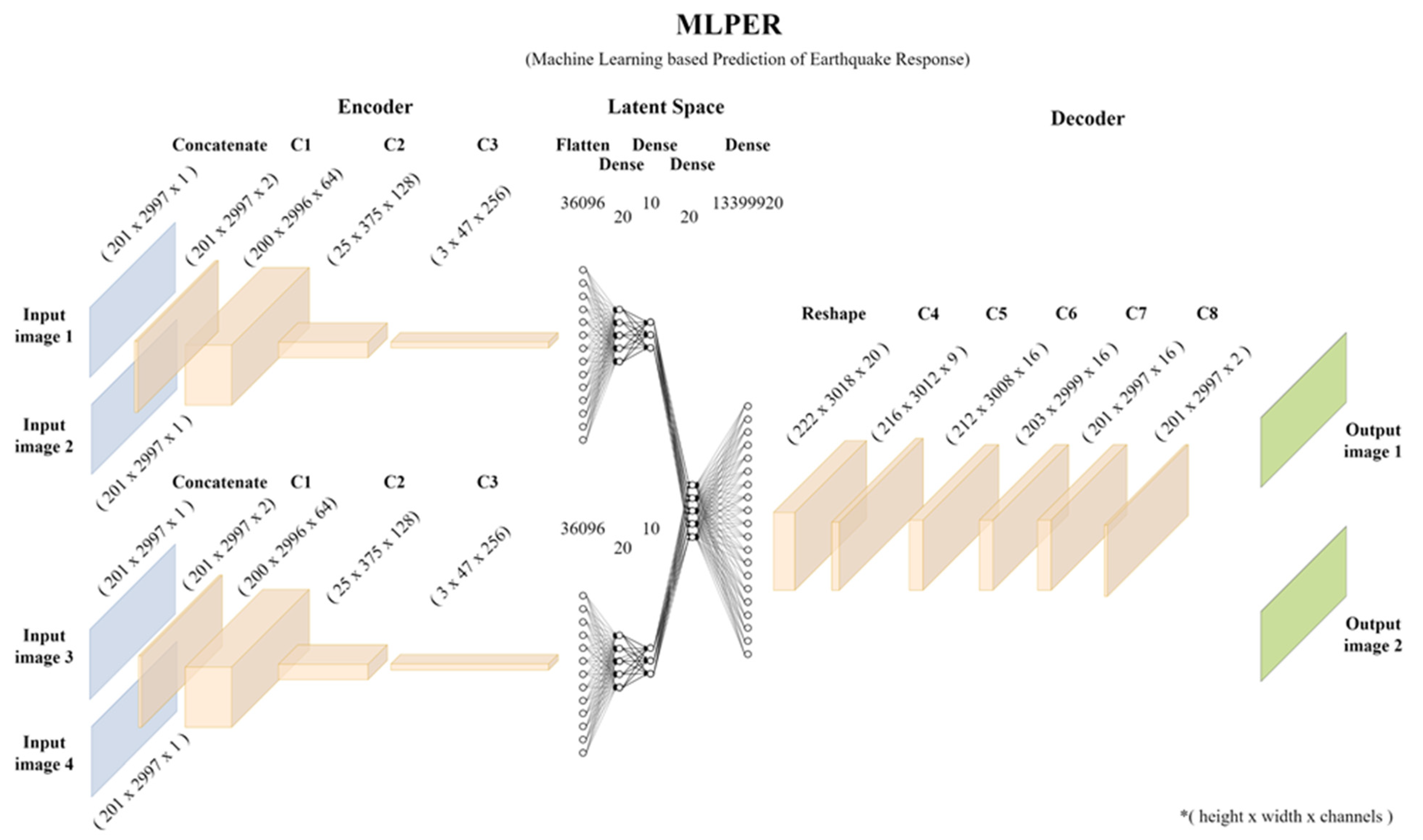
In this study, we introduce a machine learning-based model designed to forecast seismic-induced responses of MDOF systems in terms of acceleration. Referred to as MLPER, which stands for machine learning-based prediction of earthquake response in building structures, this model represents a universal approach for predicting earthquake responses in building structures. A graphical representation of the MLPER is provided in Figure 7. MLPER comprises three key stages: Encoding, Latent Space, and Decoding. As previously described in Section 3, the input to our model consists of two sets of images: amplitude and phase spectrograms representing ambient responses and earthquake data, respectively. The model’s output is a pair of images, consisting of amplitude and phase spectrograms, but this time capturing the earthquake-induced response. Each input and output image is a 2D representation with dimensions T × F, where T signifies the signal’s time duration, and F denotes the frequency values. The third dimension, the channel, represents the monochromatic color value. For amplitude spectrograms, the channel dimension represents the amplitude of acceleration (in dB) at specific frequencies and times, while for phase spectrograms, it denotes the phase angle (in pi) of the signal at particular frequencies and times. The output images follow the same format. To offer a visual overview of the MLPER model’s structure, please refer to the schematic representation in Figure 7. It is worth mentioning that all computations were conducted on an x64 PC with a 14-Core Intel® Xeon® processor with 128 GB RAM memory.
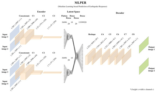
Figure 7.
The MLPER neural network model, * where in all brackets the height × width × channels of the corresponding layer is denoted.
The input format comprises four single-channel images, each sized at 2997 × 201 pixels, resulting in a tensor of shape [4, 201, 2997, 1]. We begin by splitting this tensor into four individual tensors, each having a shape of [1, 201, 2997, 1]. The next step involves the Encoding stage for each signal in the frequency domain (Table 3). Initially, the two images of shape [201, 2997, 1] are concatenated to form a tensor of shape [201, 2997, 2]. Three layers of 2D convolution (Conv2D) are applied, interspersed with Batch Normalization, ReLu activation and Spatial 2D Dropout layers. Batch Normalization standardizes the inputs of each layer, promoting a faster convergence, improved generalization, and a reduced sensitivity to parameter initialization. It also acts as a regularization method. Spatial 2D Dropout is a regularization technique that randomly sets a fraction of feature maps to zero during training, preventing overfitting and encouraging the network to learn more robust features. In the encoding stage, Spatial 2D Dropout layers were set at a 15% dropout rate, meaning 15% of randomly selected neurons in these layers were set to zero during each iteration. Following the encoding, the final layer is flattened, creating a Latent Space through several Dense layers. After the Flatten layer, two Dense layers follow with ReLu activation. At this juncture, the “paths” for the Ambient response signal and the Earthquake signal converge. This concatenation is succeeded by a Dense layer with 20 nodes and another Dense layer with 13,399,920 nodes (Table 4). Subsequently, reshaping is necessary to transition from fully connected dense layers to image-like tensors with a shape of [height, width, channels], preparing for the Decoding phase of the network. The decoding stage (Table 5) consists of 5 Conv2D layers, with Batch Normalization and ReLu layers in between. The final two Conv2D layers use a Sigmoid activation function, which constrains output values to the [0, 1] range (representing colors). No dropout layers are utilized in the decoding portion of the network. Ultimately, the tensor produced by the Decoder, as depicted in Figure 7, is reshaped into a [2, 201, 2997, 1] tensor, resulting in two output images.
Table 3.
Architecture of MLPER—Part I. ‘C’ indicates a convolutional layer (Conv2D).
Table 4.
Architecture of MLPER—Part IΙ.
Table 5.
Architecture of MLPER—Part III. ‘C’ indicates a convolutional layer (Conv2D).
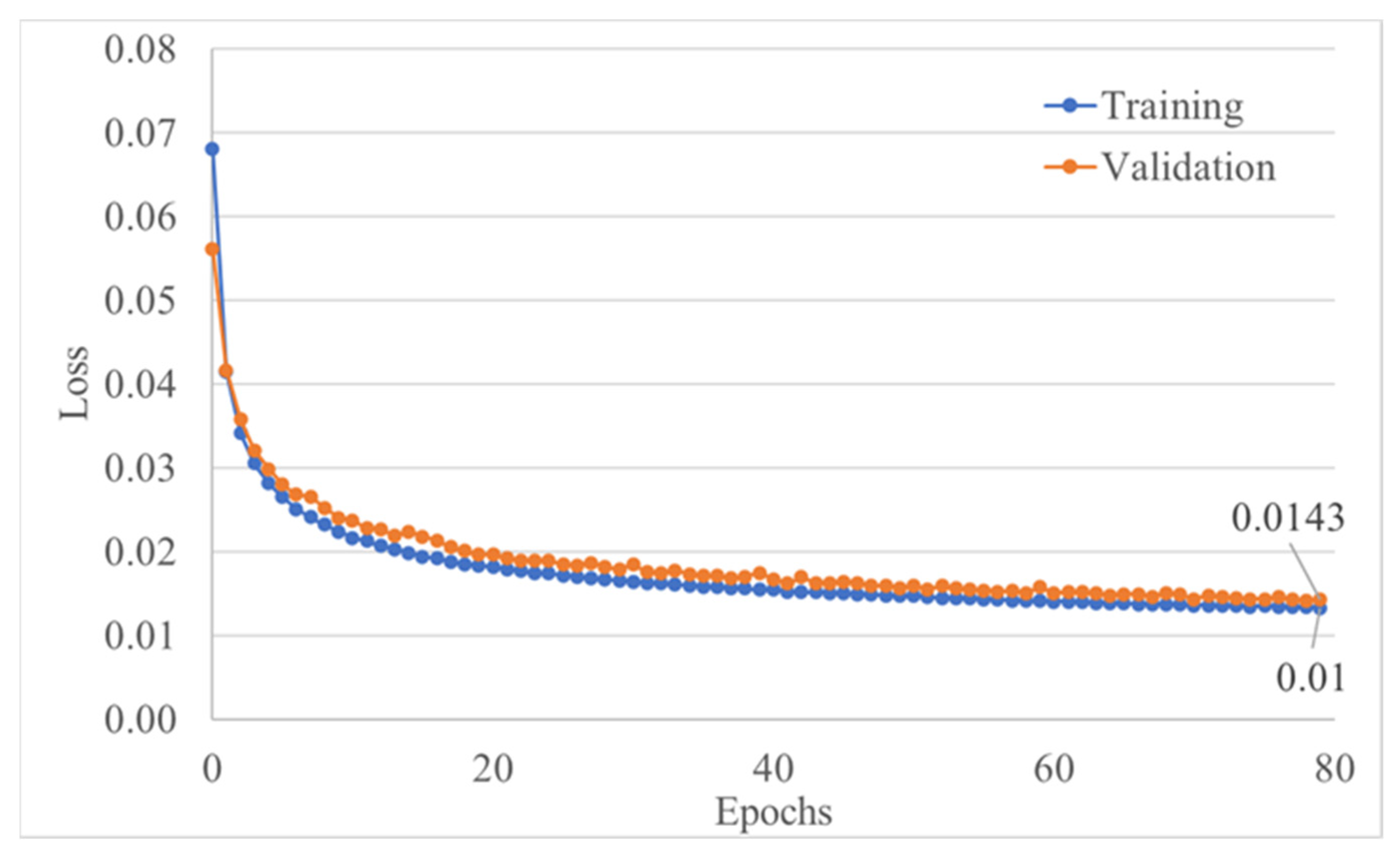
During the training process, a batch size of 12 was chosen, spanning a total of 80 epochs. The neural network employed a substantial 284,190,769 trainable parameters. To optimize the training, we utilized the Adam optimizer with the learning rate set to 0.001. Notably, in the final epoch, the training error reached 0.0133, while the prediction error amounted to 0.0143. For a comprehensive overview of the training progress, please refer to Figure 8. The selected loss function for this task was the Mean Absolute Error (MAE), computed pixel-wise by comparing the true labels and the predicted values, as defined in Equation (4).
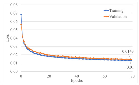
Figure 8.
Training and validation loss function value during 80 epochs.
6. Numerical Investigation—Results
As previously demonstrated, the training error was recorded at 0.0133, with the prediction error slightly higher at 0.0143. These errors represent the mean absolute errors (MAEs) computed at the pixel level between the predicted and target spectrograms, encompassing both magnitude and phase. However, as structural engineers, our primary concern lies in understanding the core problem at hand: the prediction of seismic responses in terms of acceleration. To address this, all spectrograms were transformed back into time histories, enabling us to evaluate their similarities in magnitude and trend. For this comparative analysis, we selected two key metrics: the mean absolute percentage error (MAPE) (Equation (5)) for assessing magnitude congruence and the mean directional accuracy (MDA) (Equation (6)) to gauge the directional accuracy of the time history regression between each time step. To address the challenge posed by small, near-zero values in the data, we employed a modified version of both metrics. This adaptation necessitates the introduction of a threshold mask (T) to assess signal similarities specifically for values exceeding certain magnitudes (m/sec2).
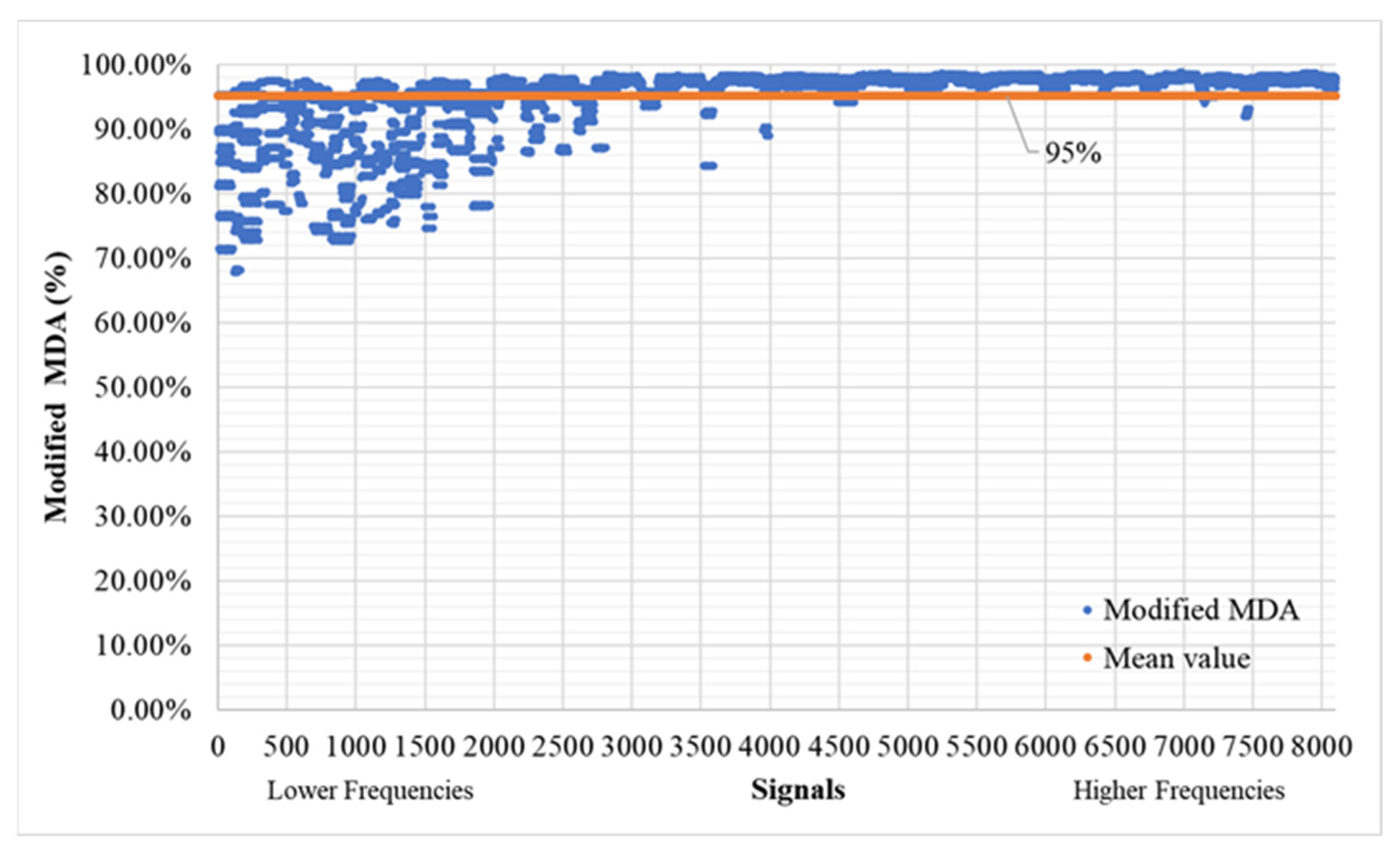
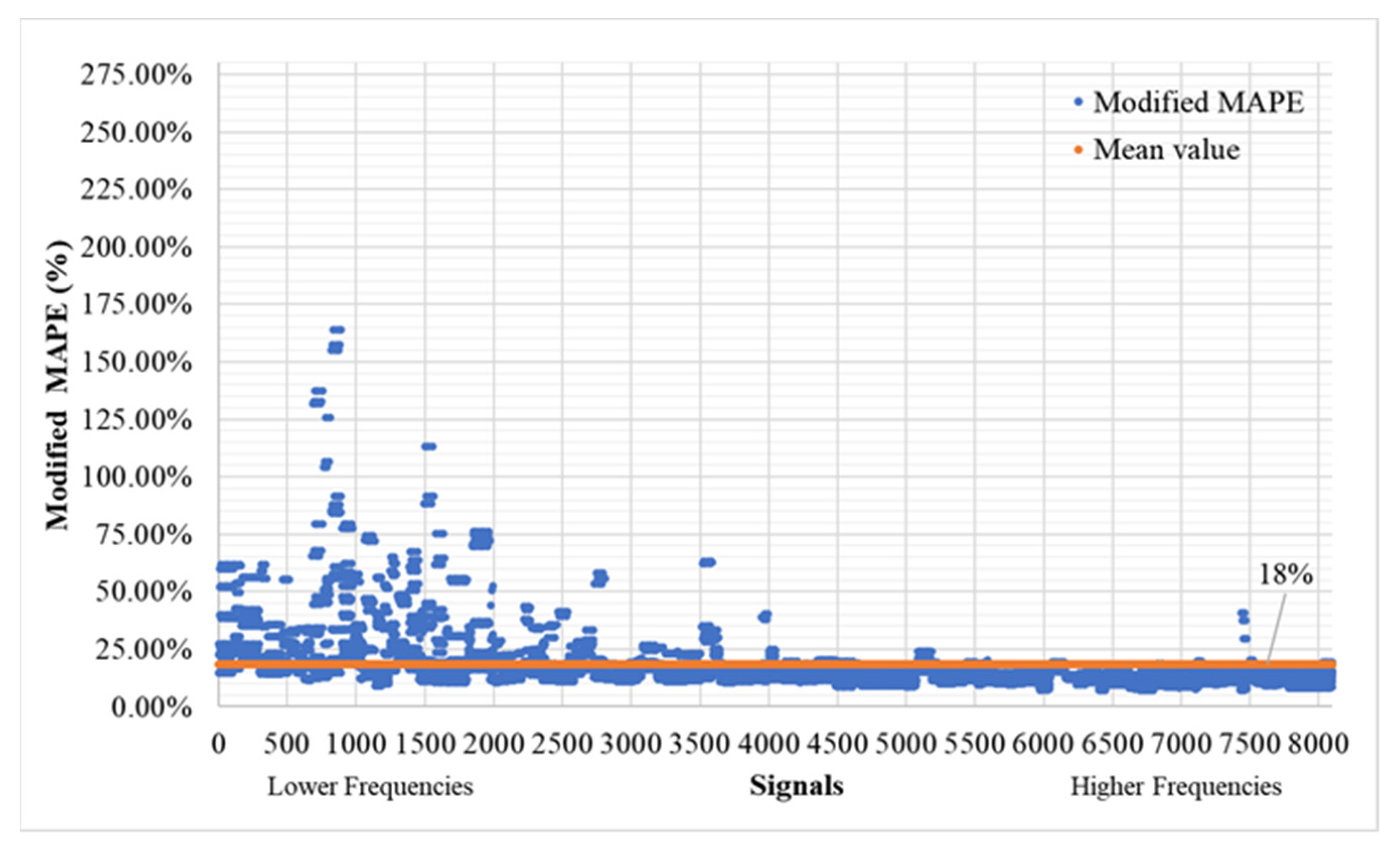
When employing small threshold mask values (T > 0.0001), the mean modified MAPE registers an average of 32%, as demonstrated in Figure 9, while the modified MDA maintains a robust average of 95%, as illustrated in Figure 10. It is worth noting that there is a more substantial deviation in accuracy observed in lower-frequency signals, suggesting potential avenues for enhancing the model’s performance. These potential modifications will be discussed in greater detail in the forthcoming chapter, Discussion. For signals with a higher frequency (≥3000 signal, equivalent to 4 Hz), the mean MAPE averages at 24.09%, and the MDA at an impressive 97.46%. To offer greater clarity to the reader regarding the extent of masking, Figure 11 and Figure 12 provide a comprehensive listing of the omitted values from the time history, which primarily include values that are in close proximity to zero, as dictated by the chosen threshold T mask.
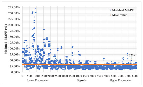
Figure 9.
Modified MAPE (T > 0.0001) of time history signals between actual and predicted for the validation set (8100 signals—300 models).

Figure 10.
Modified MDA (T > 0.0001) of time history signals between actual and predicted for the validation set (8100 signals—300 models).
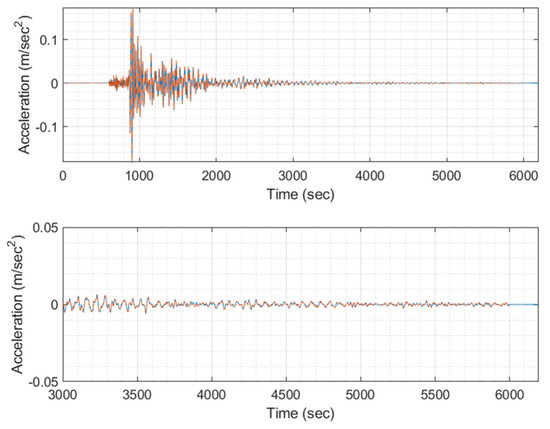
Figure 11.
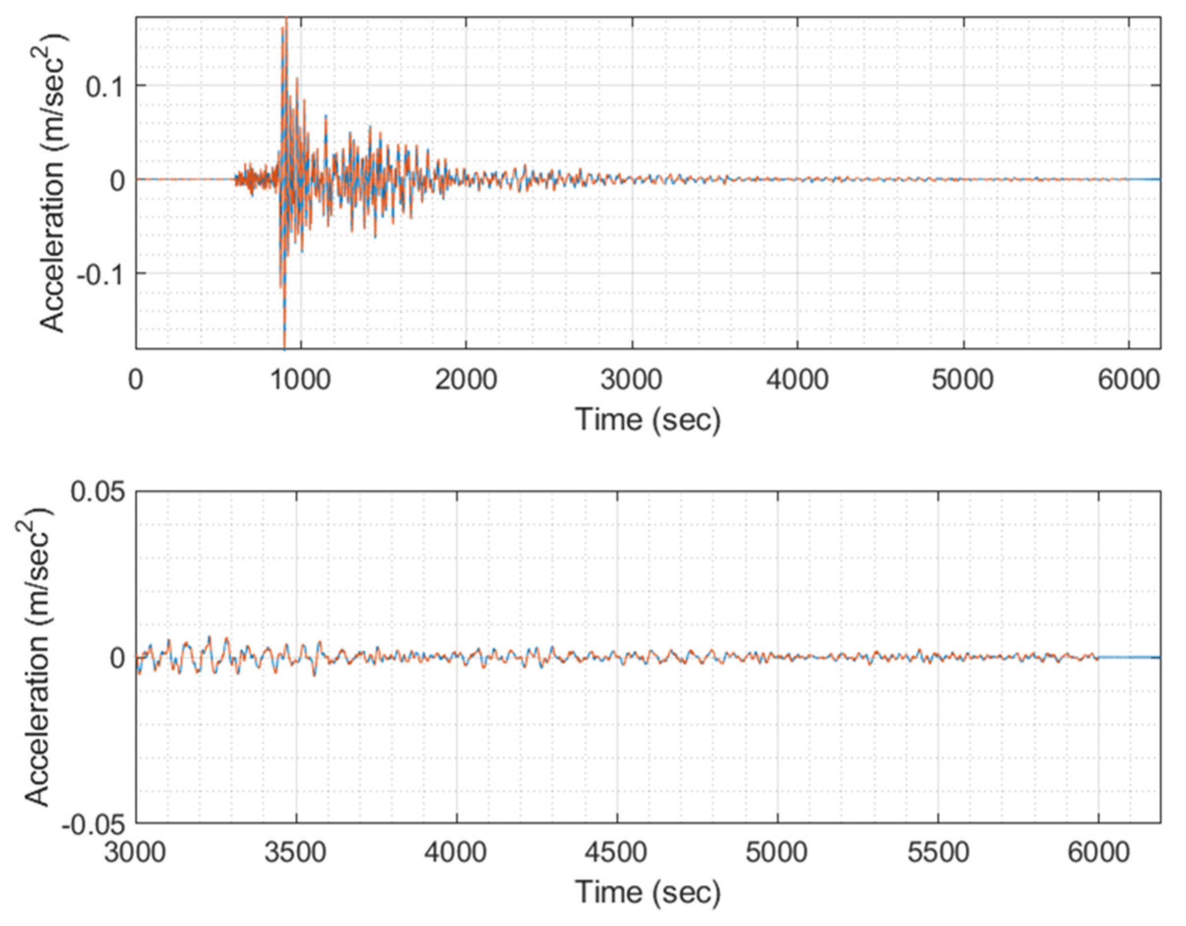
Example EQ response time history (blue) unmasked compared to the masked one (orange) for threshold T > 0.0001 of signal 1 (model #100, EQ #1).
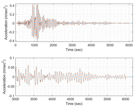
Figure 12.
Example EQ response time history (blue) unmasked compared to the masked one (orange) for threshold T > 0.0001 of signal 2 (model #100, EQ #2).
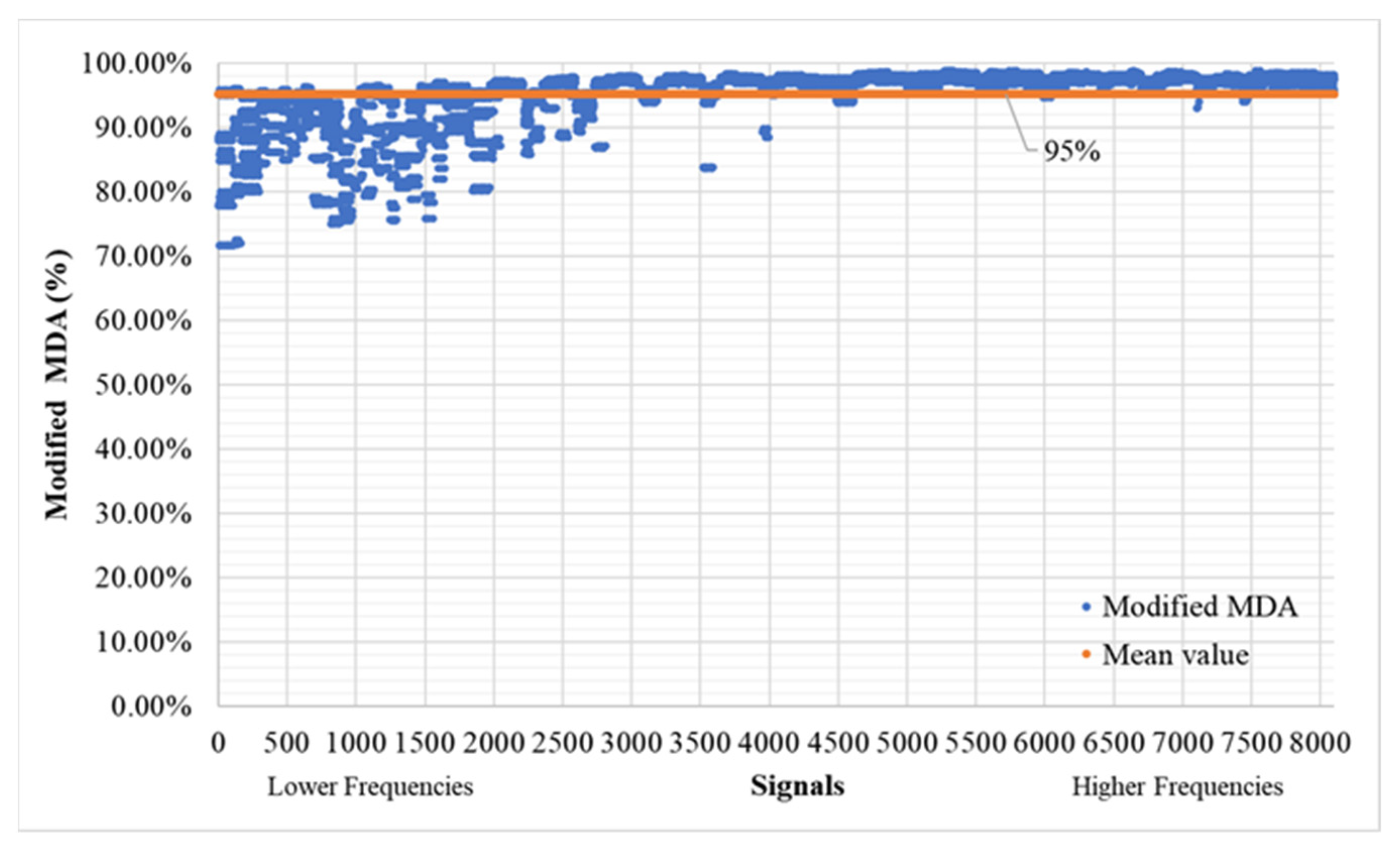
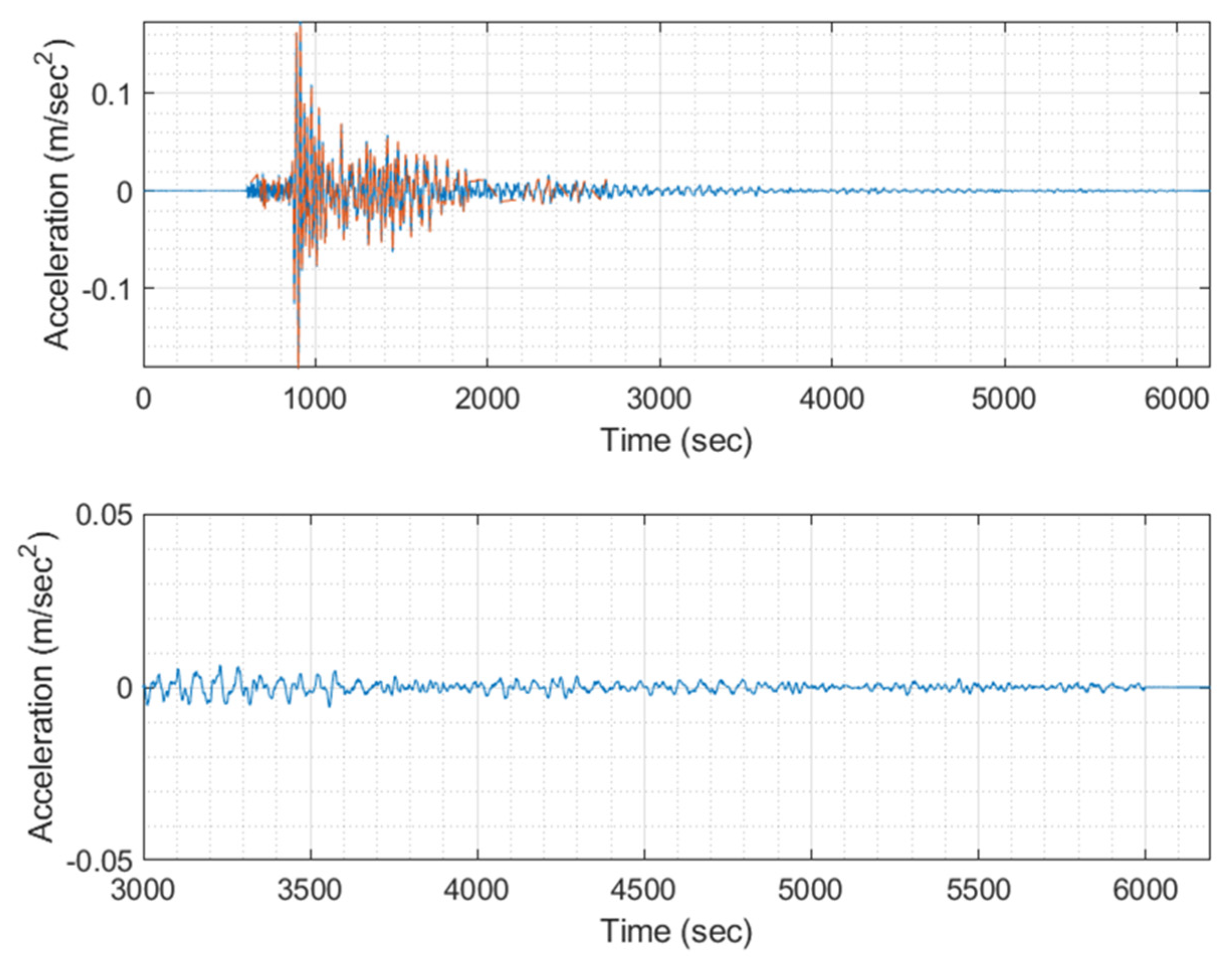
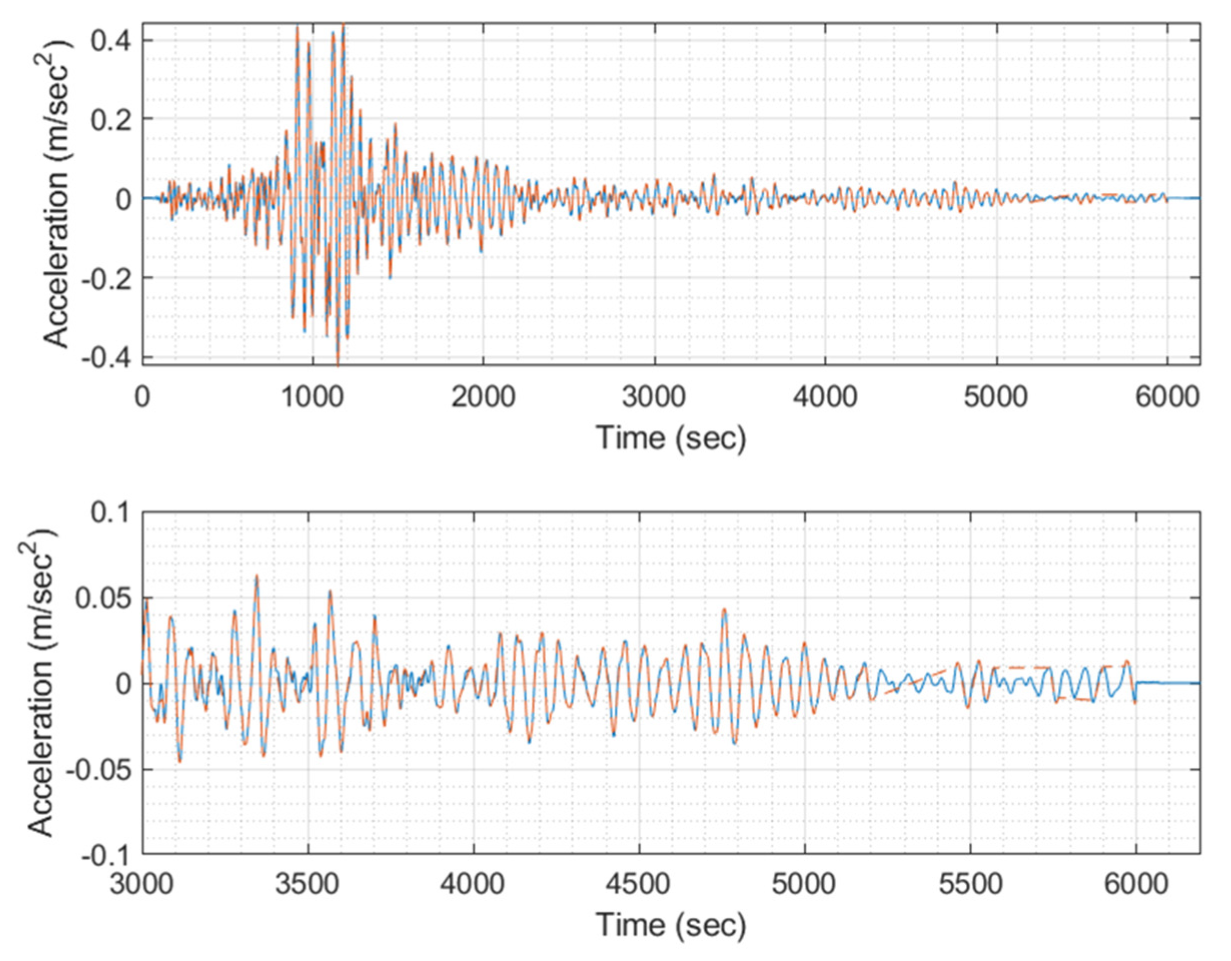
When utilizing larger threshold mask values (T > 0.01), the mean modified MAPE averages out at 18%, as indicated in Figure 13, while the modified MDA maintains a strong average of 95%, as shown in Figure 14. The deviation pattern observed remains consistent with that observed when using lower mask values, with deviations being more prominent for lower-frequency signals. For signals with a higher frequency (≥3000 signal, equivalent to 4 Hz), the mean MAPE stands at an average of 14.09%, and the MDA at an impressive 97.19%. To provide greater clarity to the reader regarding the extent of masking, Figure 15 and Figure 16 list the values from the time history that are omitted when the threshold T mask is applied. These omitted values typically correspond to those close to zero.
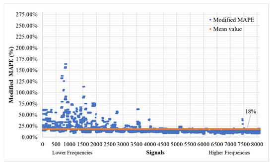
Figure 13.
Modified MAPE (T > 0.01) of time history signals between actual and predicted for the validation set (8100 signals—300 models).

Figure 14.
Modified MDA (T > 0.01) of time history signals between actual and predicted for the validation set (8100 signals—300 models).

Figure 15.
EQ response time history (blue) unmasked compared to the masked one (orange) for threshold T > 0.01 of signal 1 (model #100, EQ #1).
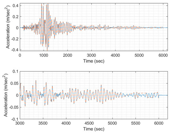
Figure 16.
EQ response time history (blue) unmasked compared to the masked one (orange) for threshold T > 0.01 of signal 2 (model #100, EQ #2).
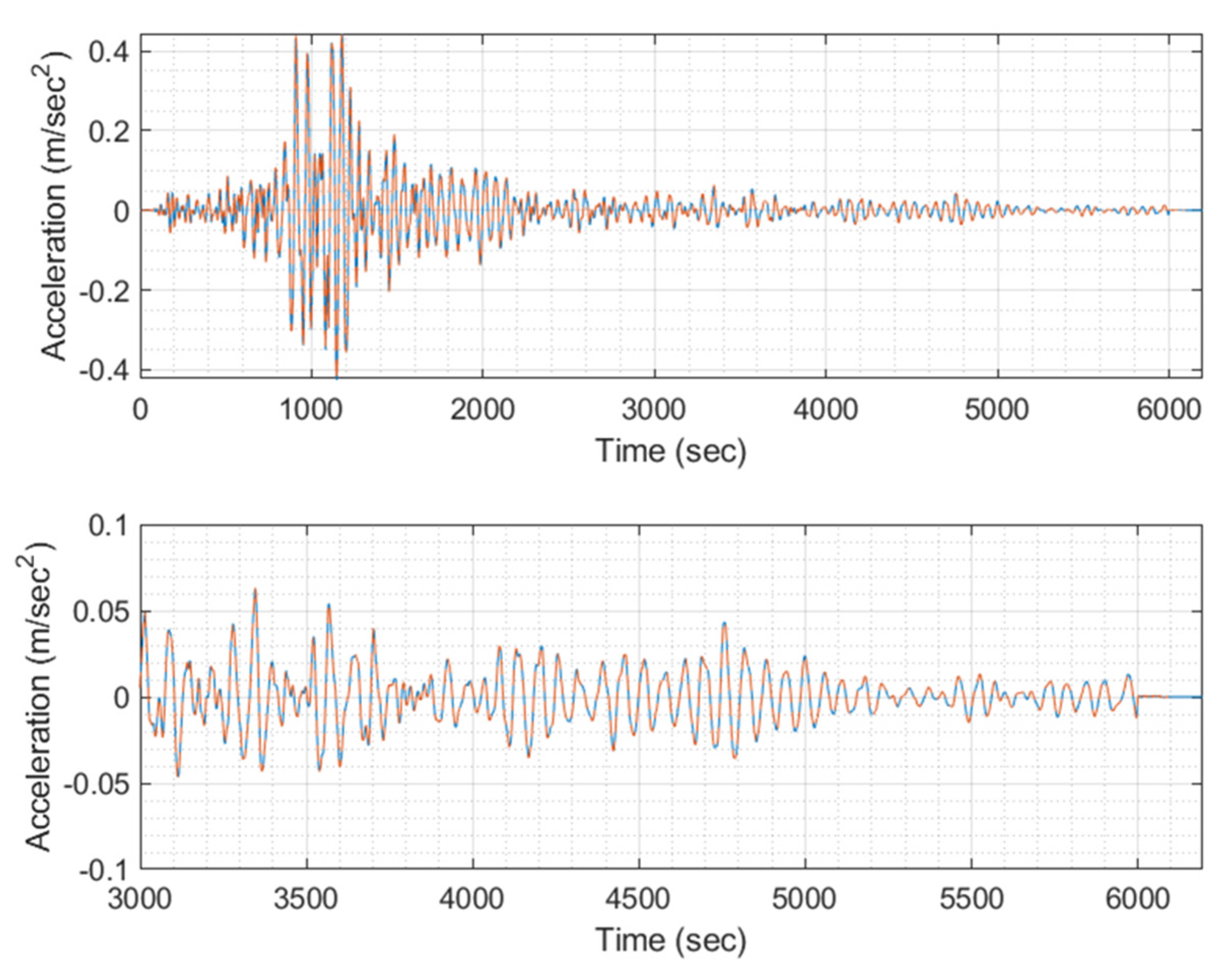
As illustrated in the figures referring to the specific test example, spanning from Figure A1, Figure A2, Figure A3, Figure A4, Figure A5, Figure A6, Figure A7, Figure A8, Figure A9, Figure A10, Figure A11, Figure A12, Figure A13, Figure A14, Figure A15, Figure A16, Figure A17 and Figure A18 in Appendix A, it is evident that the predicted response time histories for model #711 across all earthquakes (Table 2) display a certain level of similarity to the original/target responses in the specific aspects. However, this congruence is not consistent across all parameters. In terms of the phase accuracy, the model’s predictions exhibit impressive performance, with the modified MDA consistently exceeding 95%. This alignment is particularly evident when examining the “zoomed” subplots in the referenced figures, where the motion direction matches closely across timesteps for each case. One noteworthy observation pertains to the loss of accuracy in amplitude scaling, which becomes more pronounced in instances of strong acceleration values compared to weaker ones. Nevertheless, it is important to highlight that the dynamic range remains intact, as demonstrated, especially in Figure A18. The dynamic range for the threshold mask set at T = 0.0001, used for the calculations of the aforementioned metrics, reaches a maximum of 106 dB. This is approximately equivalent to an 18-bit sensor (108.4 dB), closely approaching the capabilities of a 20-bit accelerometer with a 120 dB dynamic range, without factoring in any losses attributed to electronic noise.
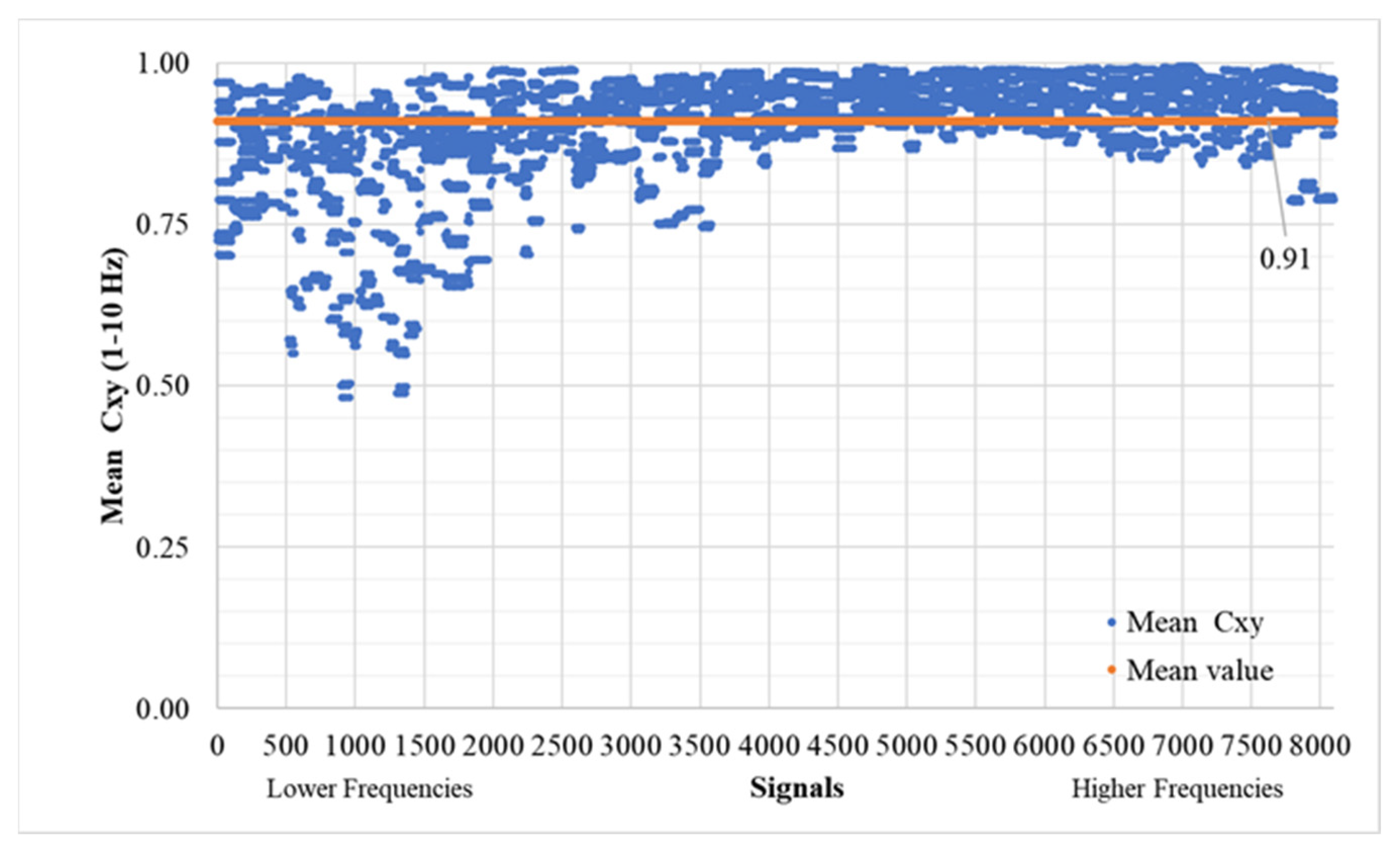
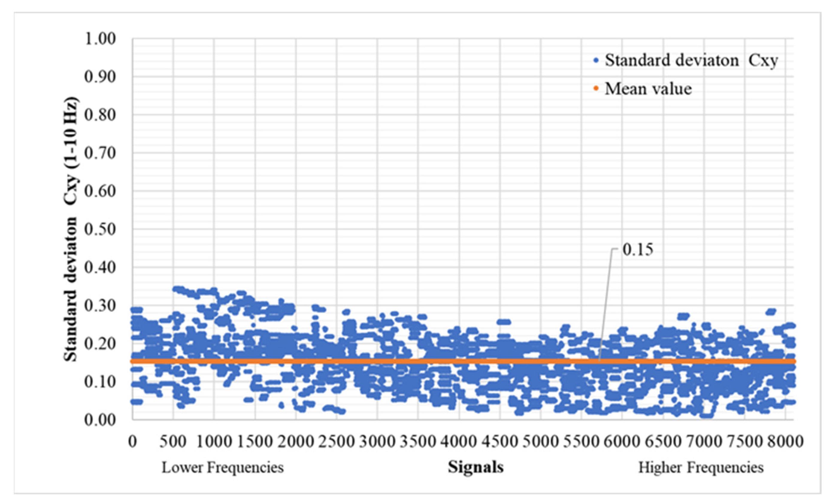
Furthermore, we conducted a comparison based on frequency spectra. Given the typically limited frequency spectrum of earthquake excitations (usually up to 10 Hz), either due to their inherent characteristics or dataset restrictions, our analysis focused on the 1–10 Hz frequency range. The initial metric involves assessing the similarity in magnitude between the Fourier spectra of the predicted and original signals, as depicted in [27,28,29]. More precisely, we calculated the magnitude-squared coherence values using (Equation (7)) for each sample, subsequently deriving the mean value from these results. In Figure 17, it is evident that the mean consistently averages at 91%, while the standard deviation of for each target/predicted signal pair averages at 15%, as illustrated in Figure 18.
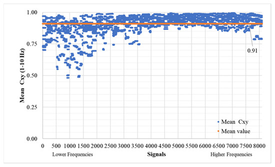
Figure 17.
Mean (T > 0.0001) of time history signals between actual and predicted for the validation set (8100 signals—300 models).

Figure 18.
Standard deviation (T > 0.0001) of time history signals between actual and predicted for the validation set (8100 signals—300 models).
As evident in the referenced figures, particularly in Figure 17, and to a somewhat lesser extent in Figure 18, there is a noticeable increase in error rates at lower frequencies. This observation can be attributed to certain aspects of the neural network architecture’s substructure. Fortunately, this issue presents an opportunity for improvement, and adjustments could be made to enhance the overall performance, similar to the excellent results already achieved for signals above 4 Hz. Specifically, for signals exceeding the 3000 ones in this context, the mean reaches an impressive 93.85%, with a corresponding standard deviation averaging at 13.46%.
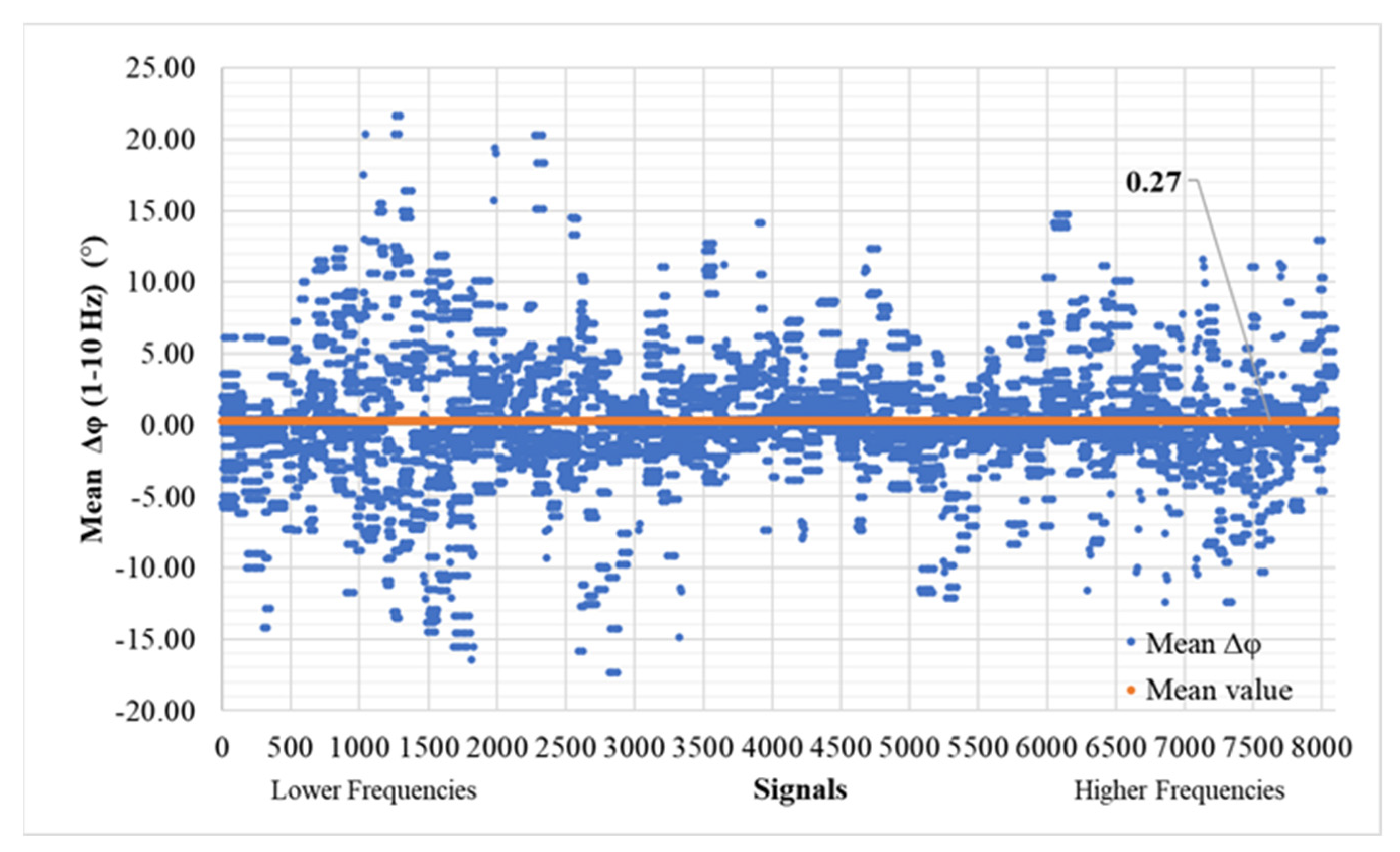
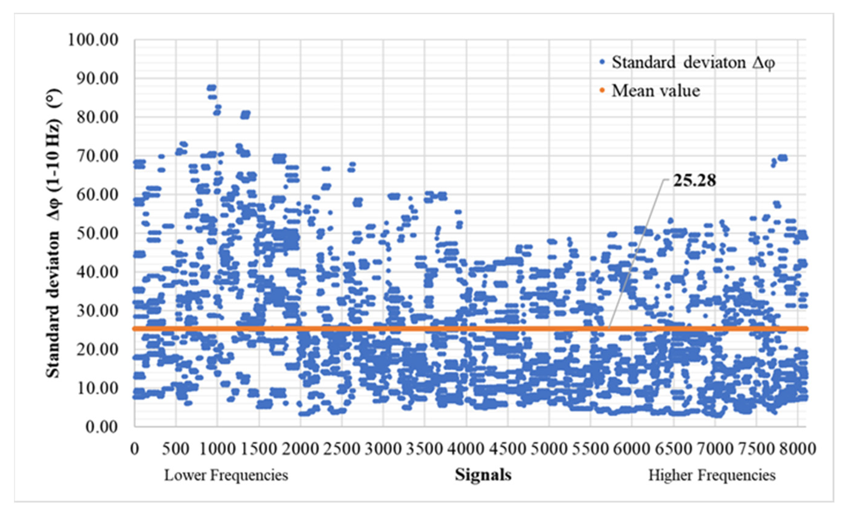
As for the phase difference (Equation (8)), the results, as shown in Figure 19 and Figure 20, are presented below. The mean phase difference consistently hovers close to zero, specifically at 0.27° across all samples. Meanwhile, the average standard deviation of for the entire dataset stands at 25.28°. It is worth noting that, unlike the MAPE, MDA, and , the error in does not exhibit a significant increase in low-frequency signals. Instead, its standard deviation shows a slightly wider dispersion at lower frequencies, although it does not dominate the overall pattern.
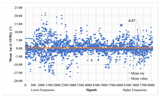
Figure 19.
Mean phase difference () (T > 0.0001) of time history signals between actual and predicted for the validation set (8100 signals—300 models).

Figure 20.
Standard deviation phase difference () (T > 0.0001) of time history signals between actual and predicted for the validation set (8100 signals—300 models).
7. Discussion
In this study, we introduce a neural network model designed to predict the response of multi-degree-of-freedom (MDOF) systems when subjected to seismic events, specifically targeting the nth degree of freedom (top storey translational degree of freedom), all without the need to perform complex nonlinear time history analyses. This study serves as a pivotal foundational milestone in our pursuit of a larger goal: achieving precise earthquake response predictions for all types of buildings, while comprehensively considering factors such as site effects, second-order effects, and deviations from bilinear stiffness behavior. To realize this overarching objective, we intend to leverage various means, including the accumulation of insights derived from real-world observations and numerically generated datasets.
Our prediction methodology utilizes time history images of ambient responses of MDOF systems in conjunction with the target earthquake event. The model then forecasts the response of the MDOF system’s top floor, typically the concrete floor exhibiting diaphragm behavior. In evaluating our model’s performance in the time domain, we find generally favorable results. However, it is worth noting that outliers in the predictions exhibit an average error rate of 14% (see Figure 21); for signals over 3000 ID, this error becomes equal to 11.10%. This issue could potentially be mitigated through the implementation of a weighted loss function, which would penalize inaccuracies in extreme values (0 or 1) more severely. Further analysis reveals that the model’s error variation is more pronounced for lower-frequency samples, likely stemming from the chosen decoding layers of the network (see Table 5). Despite using strides with small kernel sizes of (2,2) and (4,4), it appears that the model struggles to capture the low-frequency attributes of motion in the signals. Consequently, future research should focus on enhancing the network’s ability to extract information from input images, particularly at lower frequencies.
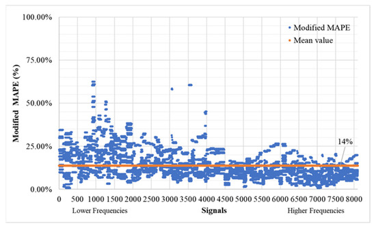
Figure 21.
Modified MAPE (T > 0.75 Max Of Each Timeseries) of time history signals between actual and predicted for the validation set (8100 signals—300 models) for the validation of outliers’ performance.
Our study’s evaluation metrics, including modified mean absolute percentage error (MAPE), MDA, magnitude-square coherence values, and phase differences (), collectively indicate promising performance from the proposed network. It successfully predicts earthquake responses for various MDOF systems with efficiency and accuracy, relying solely on acceleration time history images.
Author Contributions
Conceptualization, S.D. and N.D.L.; methodology, S.D. and N.D.L.; software, S.D.; validation, S.D.; formal analysis, S.D.; investigation, S.D.; writing—original draft preparation, S.D. and N.D.L.; writing—review and editing, S.D. and N.D.L.; visualization, S.D.; supervision, N.D.L.; project administration, N.D.L. All authors have read and agreed to the published version of the manuscript.
Funding
This research has been financed by the IMSFARE project: “Advanced Information Modelling for SAFER structures against manmade hazards”, (Project Number: 00356).
Institutional Review Board Statement
Not applicable.
Informed Consent Statement
Not applicable.
Data Availability Statement
The data used in the study are available from the authors and can be shared upon reasonable request.
Acknowledgments
The research was supported by the Hellenic Foundation for Research and Innovation (H.F.R.I.) under the “2nd Call for H.F.R.I. Research Projects to support Post-Doctoral Researchers”, and the IMSFARE project: “Advanced Information Modelling for SAFER structures against manmade hazards”, (Project Number: 00356).
Conflicts of Interest
The authors declare no conflict of interest.
Appendix A
Predicted response time histories for model #711 (6.5 Hz, 2 stories, and 1.2 Mass reference ratio) across all earthquakes. This sample, as with the others, displays a certain level of similarity to the original/target responses in specific aspects. In each of the following figures, the response of the specific sample model is shown, both in frequency and time domains for each of the earthquakes. Meanwhile, MDOF models’ IDs are increment values of the combination of frequency, number of stories, and mass reference ratio. The model naming is shown in the following table.
Table A1.
MDOF models’ labeling.
Table A1.
MDOF models’ labeling.
| ID | Frequency (Hz) | Stories | Mass Reference Ratio |
|---|---|---|---|
| 1 | 1 | 1 | 0.8 |
| 2 | 1 | 1 | 0.85 |
| . | . | . | . |
| . | . | . | . |
| . | . | . | . |
| 62 | 1 | 7 | 1.15 |
| 63 | 1 | 7 | 1.2 |
| . | . | . | . |
| . | . | . | . |
| . | . | . | . |
| 66 | 1.5 | 1 | 0.9 |

Figure A1.
A sample of input/output set of images for training, with (a) EQ response phase target (signal 5995), (b) EQ response phase predicted (signal 5995), (c) EQ response magnitude target (signal 5995), and (d) EQ response magnitude predicted (signal 5995).
Figure A1.
A sample of input/output set of images for training, with (a) EQ response phase target (signal 5995), (b) EQ response phase predicted (signal 5995), (c) EQ response magnitude target (signal 5995), and (d) EQ response magnitude predicted (signal 5995).
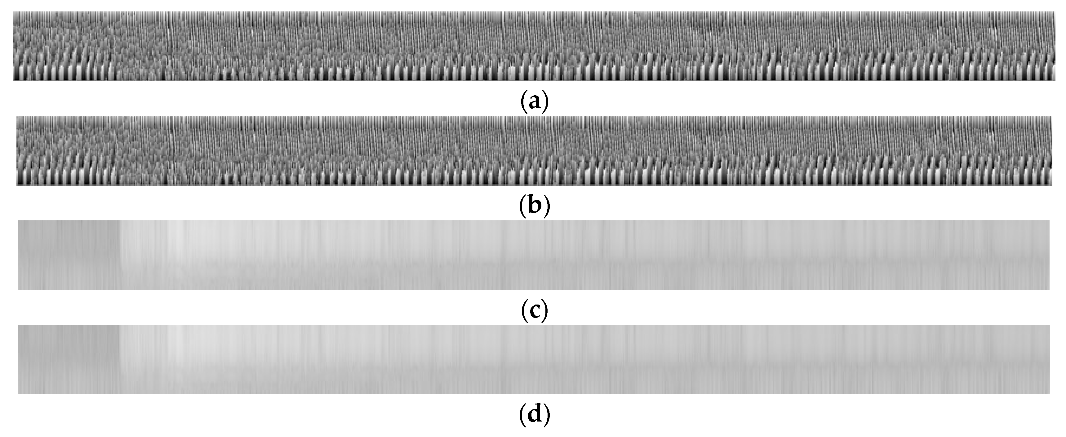
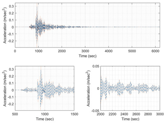
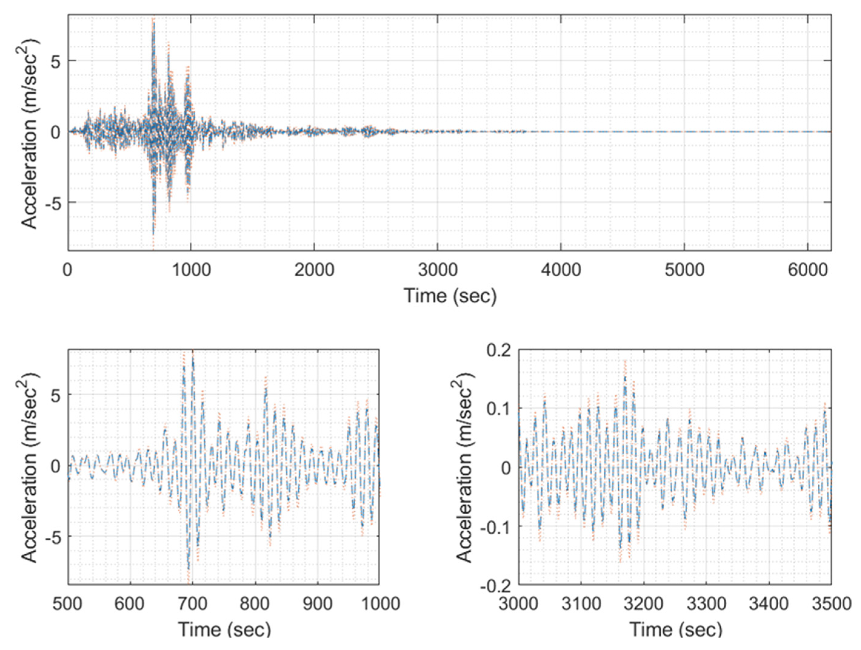
Figure A2.
Predicted EQ response time history (blue) compared to the target one (orange) of signal 5995 (model #711, EQ #1).
Figure A2.
Predicted EQ response time history (blue) compared to the target one (orange) of signal 5995 (model #711, EQ #1).
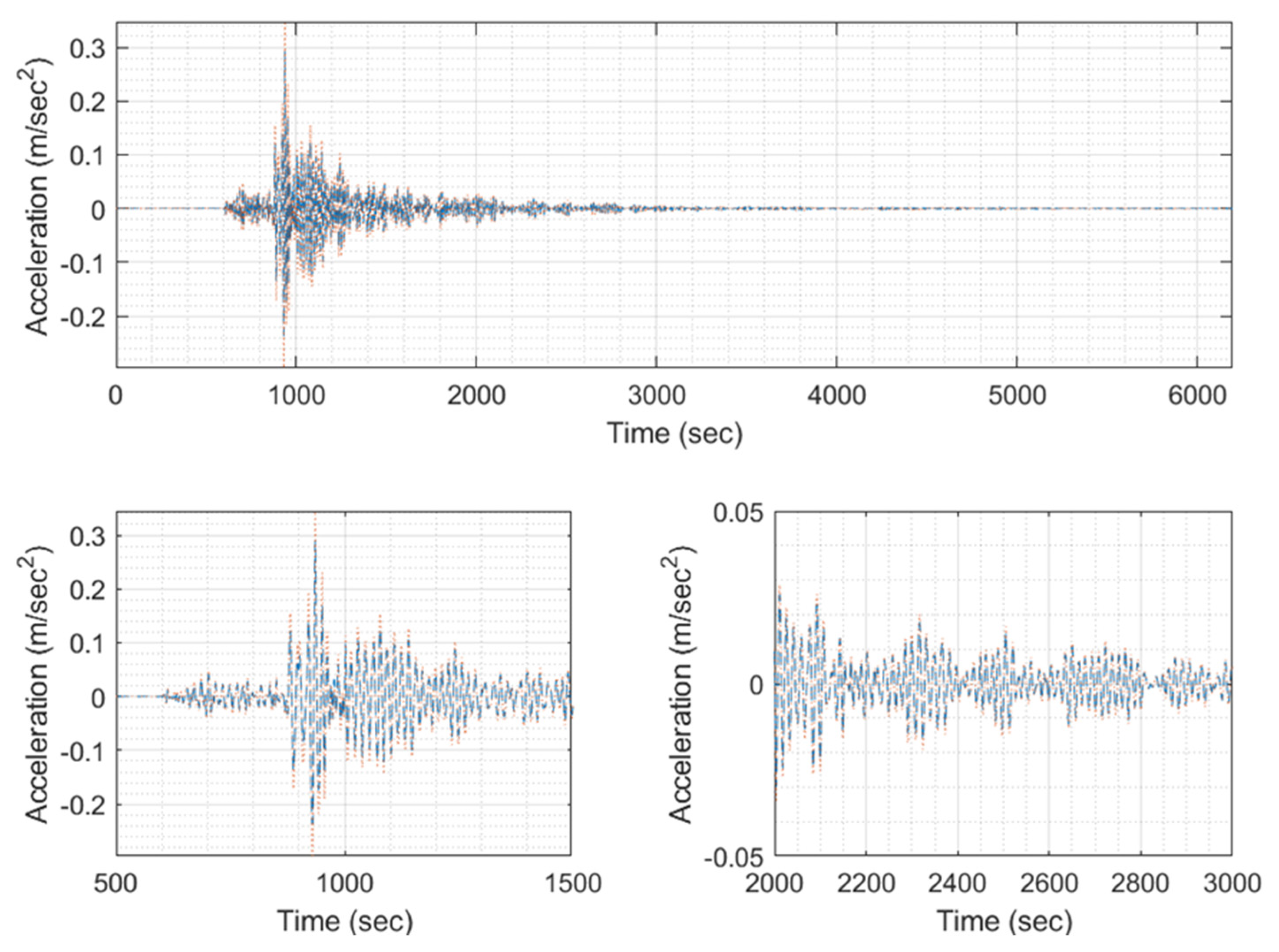

Figure A3.
A sample of input/output set of images for training, with (a) EQ response phase target (signal 5996), (b) EQ response phase predicted (signal 5996), (c) EQ response magnitude target (signal 5996), and (d) EQ response magnitude predicted (signal 5996).
Figure A3.
A sample of input/output set of images for training, with (a) EQ response phase target (signal 5996), (b) EQ response phase predicted (signal 5996), (c) EQ response magnitude target (signal 5996), and (d) EQ response magnitude predicted (signal 5996).
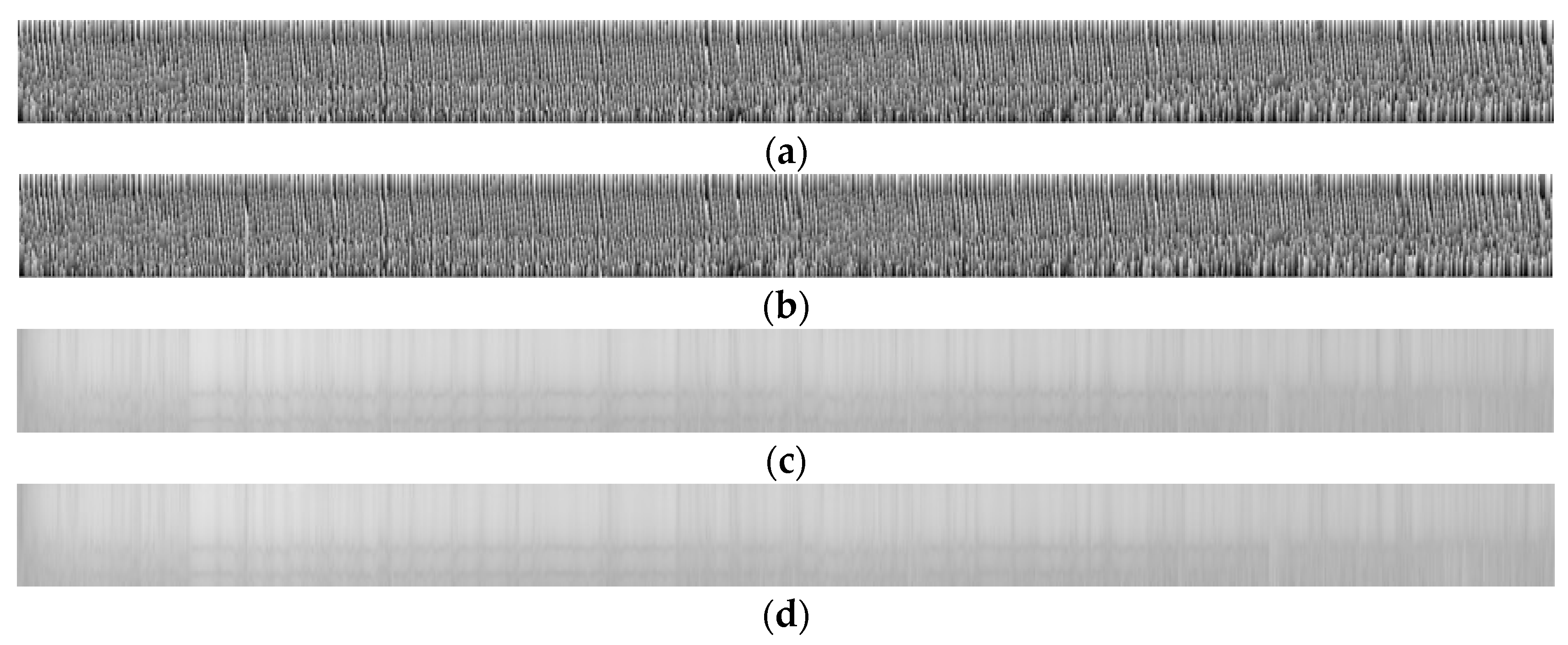
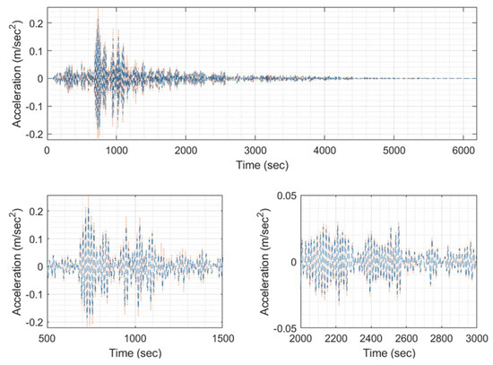
Figure A4.
Predicted EQ response time history (blue) compared to the target one (orange) of signal 5996 (model #711, EQ #2).
Figure A4.
Predicted EQ response time history (blue) compared to the target one (orange) of signal 5996 (model #711, EQ #2).
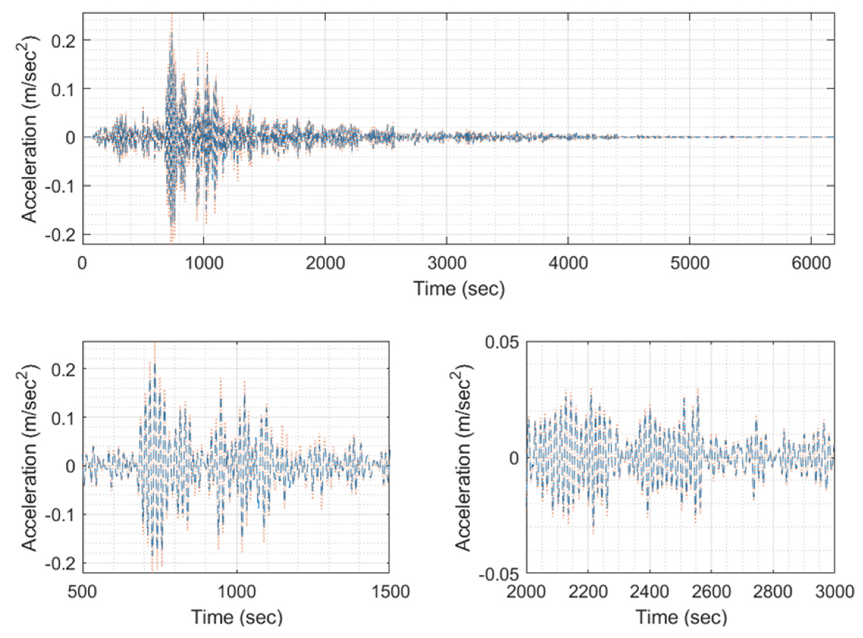
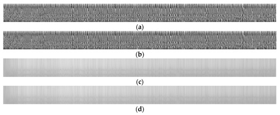
Figure A5.
A sample of input/output set of images for training, with (a) EQ response phase target (signal 5997), (b) EQ response phase predicted (signal 5997), (c) EQ response magnitude target (signal 5997), and (d) EQ response magnitude predicted (signal 5997).
Figure A5.
A sample of input/output set of images for training, with (a) EQ response phase target (signal 5997), (b) EQ response phase predicted (signal 5997), (c) EQ response magnitude target (signal 5997), and (d) EQ response magnitude predicted (signal 5997).
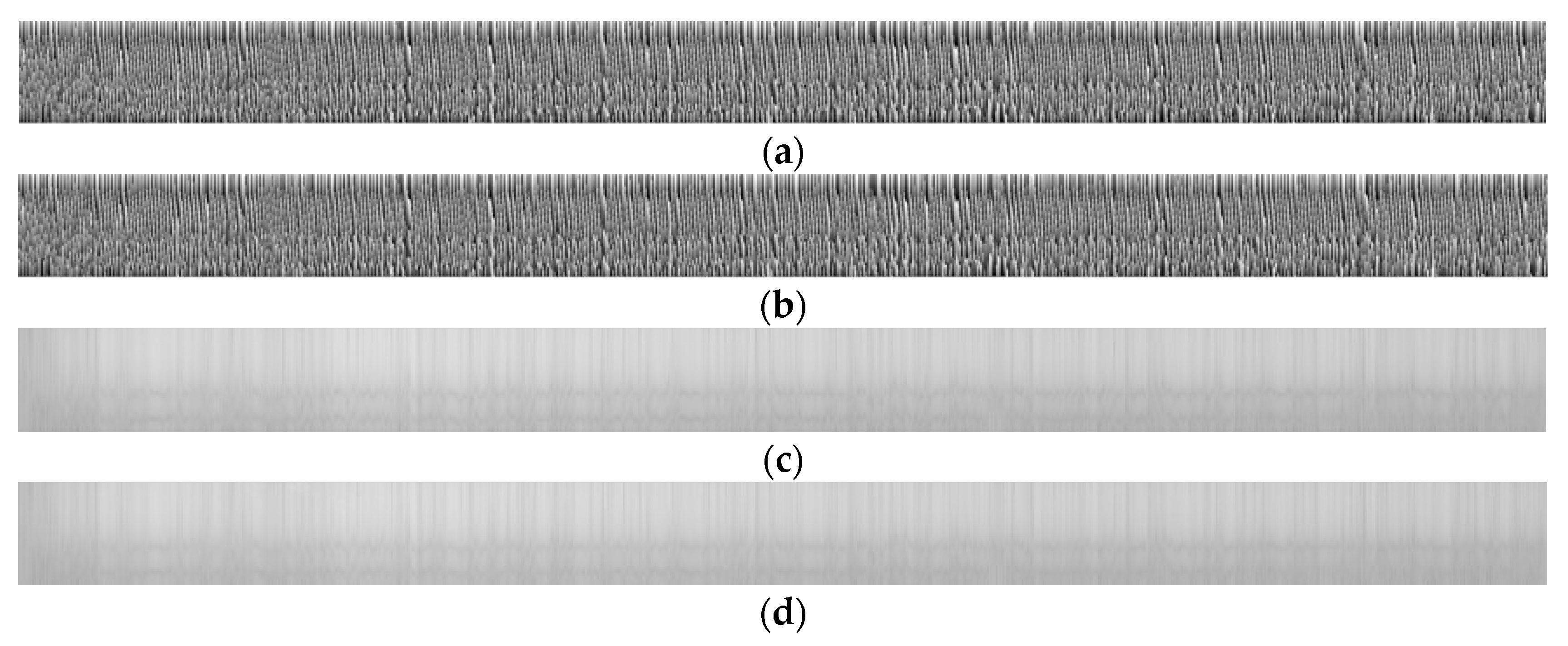
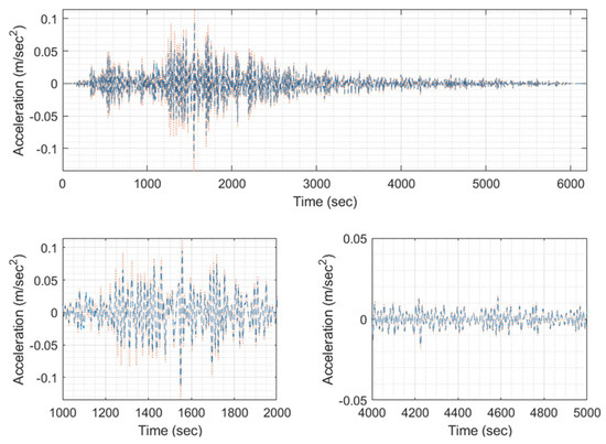
Figure A6.
Predicted EQ response time history (blue) compared to the target one (orange) of signal 5997 (model #711, EQ #3).
Figure A6.
Predicted EQ response time history (blue) compared to the target one (orange) of signal 5997 (model #711, EQ #3).
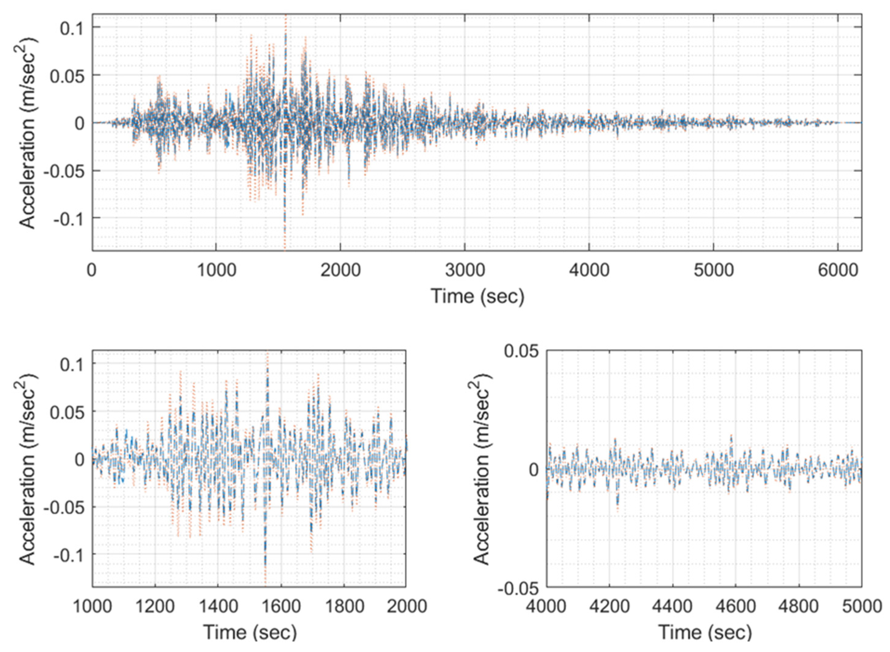

Figure A7.
A sample of input/output set of images for training, with (a) EQ response phase target (signal 5998), (b) EQ response phase predicted (signal 5998), (c) EQ response magnitude target (signal 5998), and (d) EQ response magnitude predicted (signal 5998).
Figure A7.
A sample of input/output set of images for training, with (a) EQ response phase target (signal 5998), (b) EQ response phase predicted (signal 5998), (c) EQ response magnitude target (signal 5998), and (d) EQ response magnitude predicted (signal 5998).
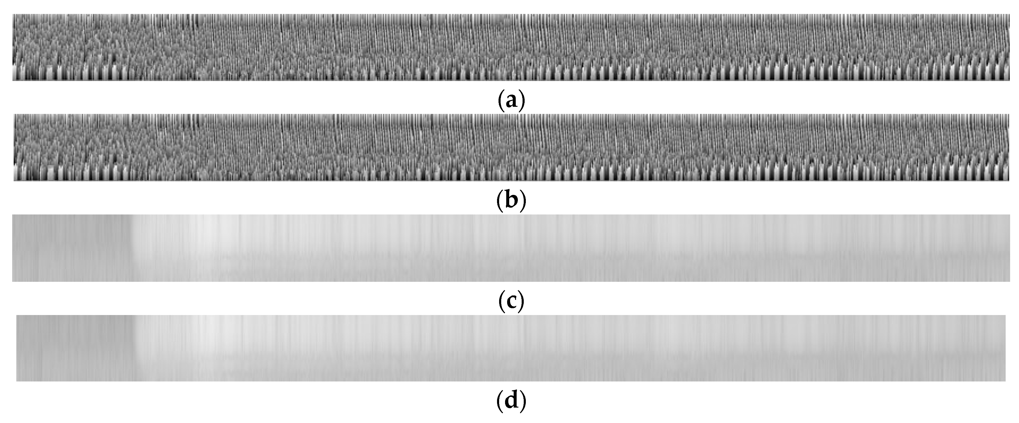
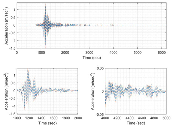
Figure A8.
Predicted EQ response time history (blue) compared to the target one (orange) of signal 5998 (model #711, EQ #4).
Figure A8.
Predicted EQ response time history (blue) compared to the target one (orange) of signal 5998 (model #711, EQ #4).
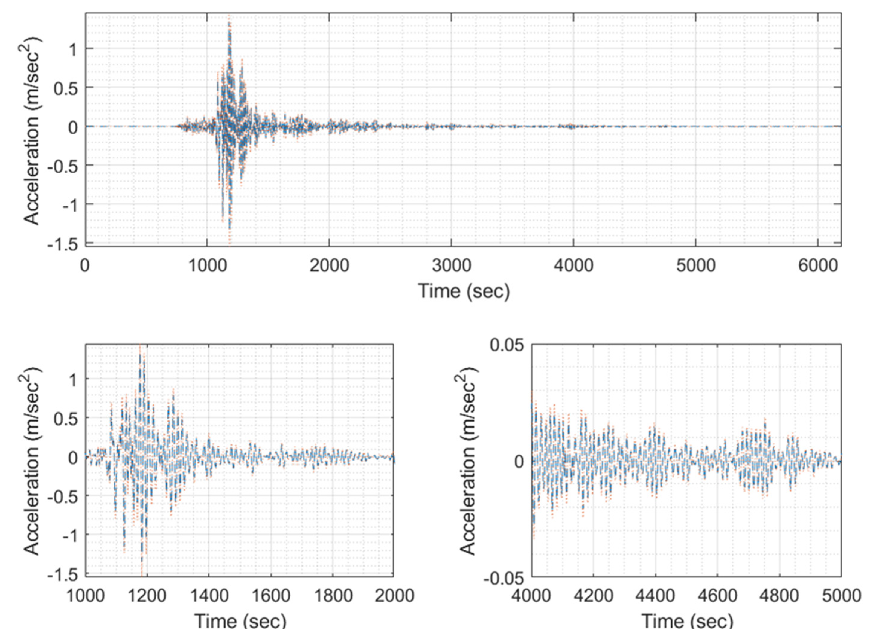
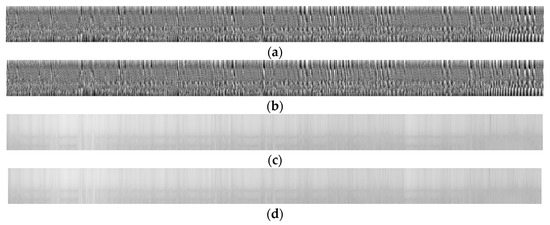
Figure A9.
A sample of input/output set of images for training, with (a) EQ response phase target (signal 5999), (b) EQ response phase predicted (signal 5999), (c) EQ response magnitude target (signal 5999), ad (d) EQ response magnitude predicted (signal 5999).
Figure A9.
A sample of input/output set of images for training, with (a) EQ response phase target (signal 5999), (b) EQ response phase predicted (signal 5999), (c) EQ response magnitude target (signal 5999), ad (d) EQ response magnitude predicted (signal 5999).
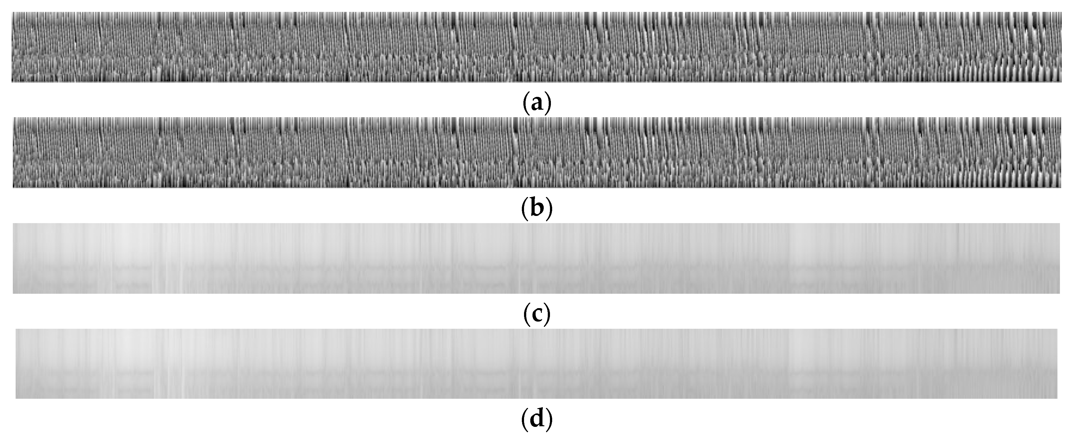
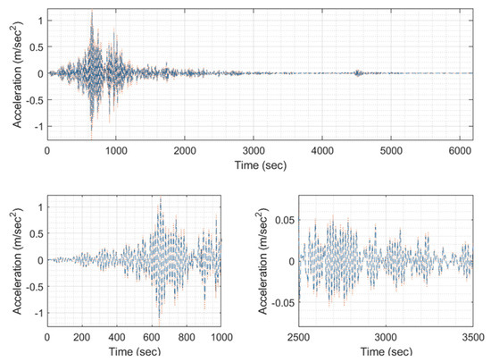
Figure A10.
Predicted EQ response time history (blue) compared to the target one (orange) of signal 5999 (model #711, EQ #5).
Figure A10.
Predicted EQ response time history (blue) compared to the target one (orange) of signal 5999 (model #711, EQ #5).
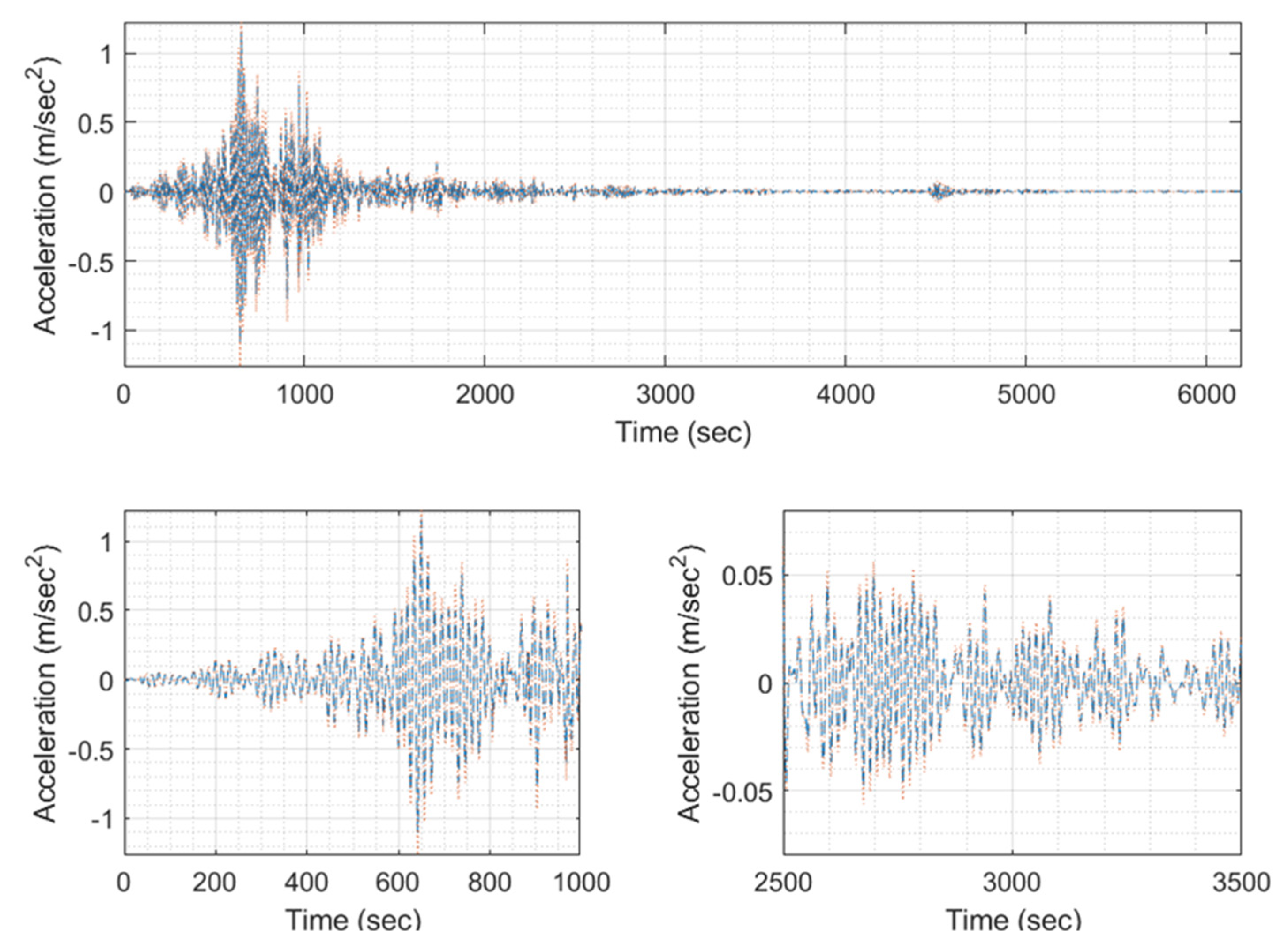
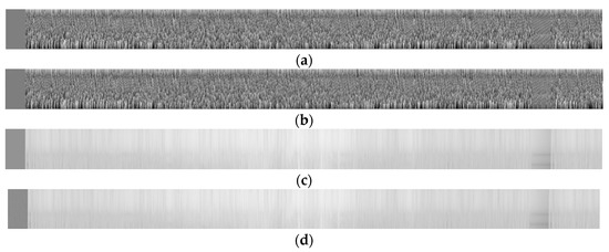
Figure A11.
A sample of input/output set of images for training, with (a) EQ response phase target (signal 6000), (b) EQ response phase predicted (signal 6000), (c) EQ response magnitude target (signal 6000), and (d) EQ response magnitude predicted (signal 6000).
Figure A11.
A sample of input/output set of images for training, with (a) EQ response phase target (signal 6000), (b) EQ response phase predicted (signal 6000), (c) EQ response magnitude target (signal 6000), and (d) EQ response magnitude predicted (signal 6000).
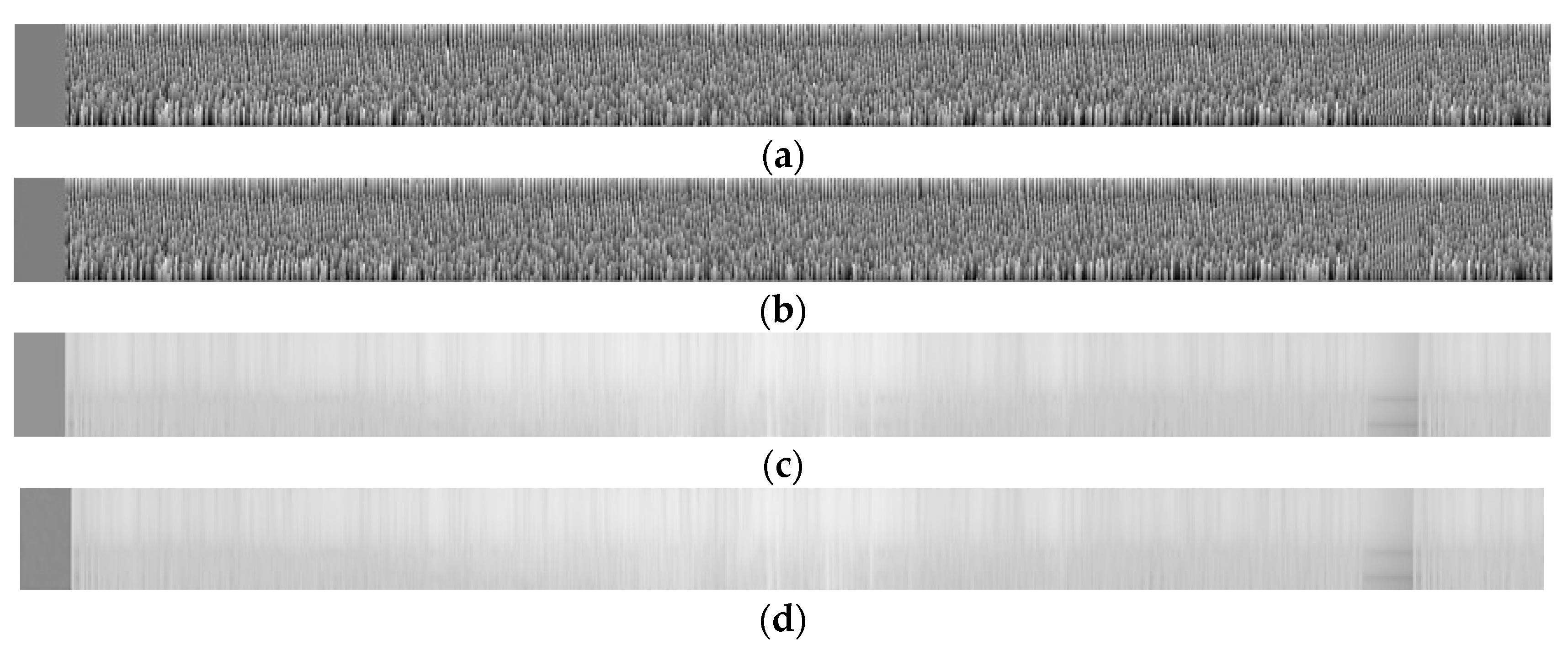
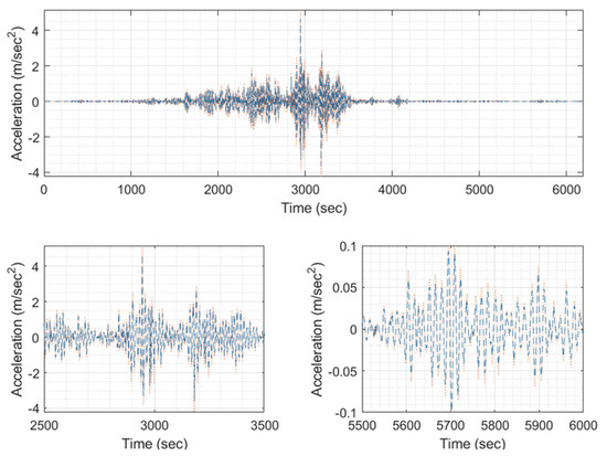
Figure A12.
Predicted EQ response time history (blue) compared to the target one (orange) of signal 6000 (model #711, EQ #6).
Figure A12.
Predicted EQ response time history (blue) compared to the target one (orange) of signal 6000 (model #711, EQ #6).
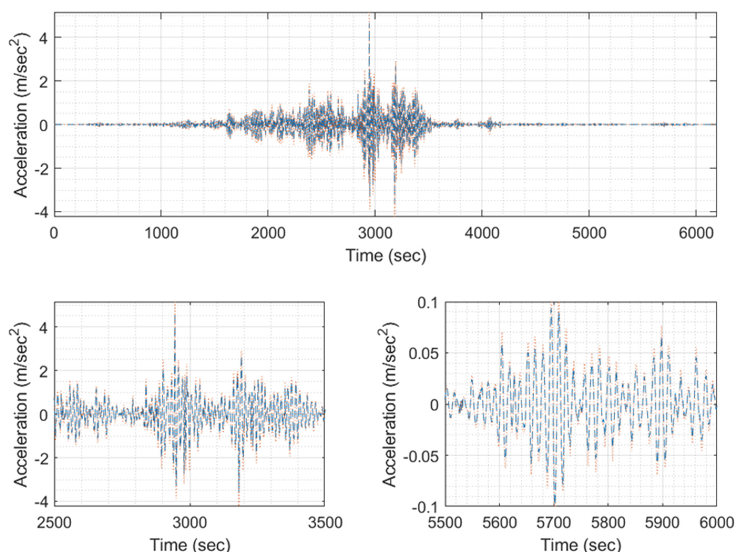
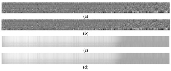
Figure A13.
A sample of input/output set of images for training, with (a) EQ response phase target (signal 6001), (b) EQ response phase predicted (signal 6001), (c) EQ response magnitude target (signal 6001), and (d) EQ response magnitude predicted (signal 6001).
Figure A13.
A sample of input/output set of images for training, with (a) EQ response phase target (signal 6001), (b) EQ response phase predicted (signal 6001), (c) EQ response magnitude target (signal 6001), and (d) EQ response magnitude predicted (signal 6001).

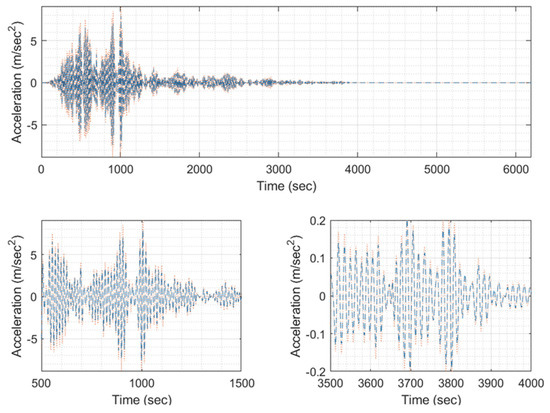
Figure A14.
Predicted EQ response time history (blue) compared to the target one (orange) of signal 6001 (model #711, EQ #7).
Figure A14.
Predicted EQ response time history (blue) compared to the target one (orange) of signal 6001 (model #711, EQ #7).
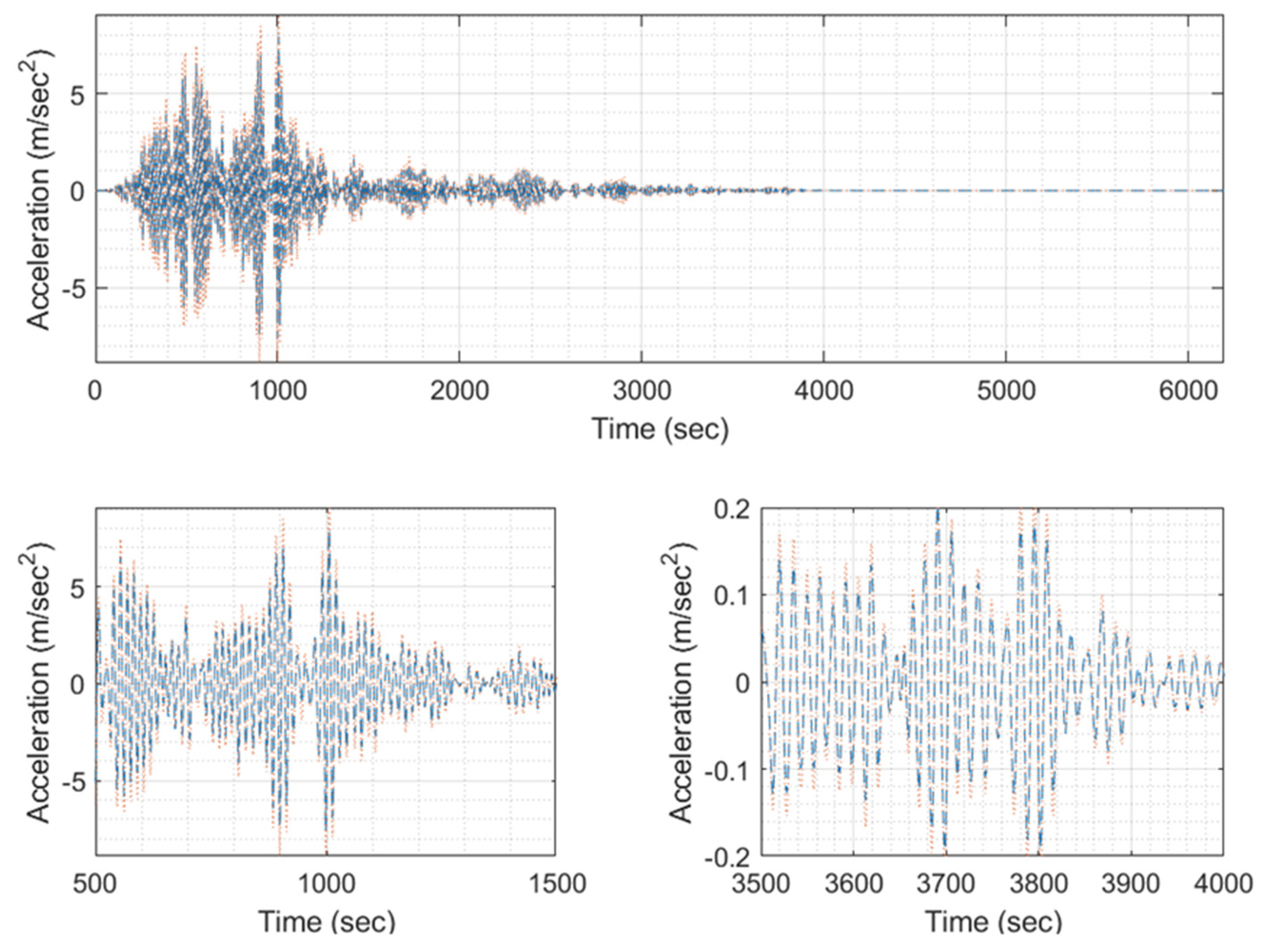
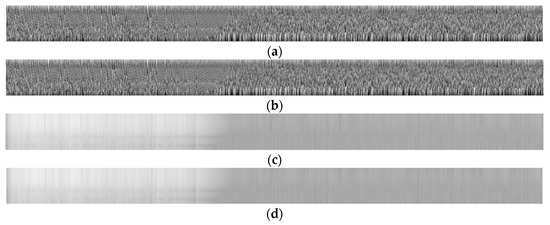
Figure A15.
A sample of input/output set of images for training, with (a) EQ response phase target (signal 6002), (b) EQ response phase predicted (signal 6002), (c) EQ response magnitude target (signal 6002), and (d) EQ response magnitude predicted (signal 6002).
Figure A15.
A sample of input/output set of images for training, with (a) EQ response phase target (signal 6002), (b) EQ response phase predicted (signal 6002), (c) EQ response magnitude target (signal 6002), and (d) EQ response magnitude predicted (signal 6002).
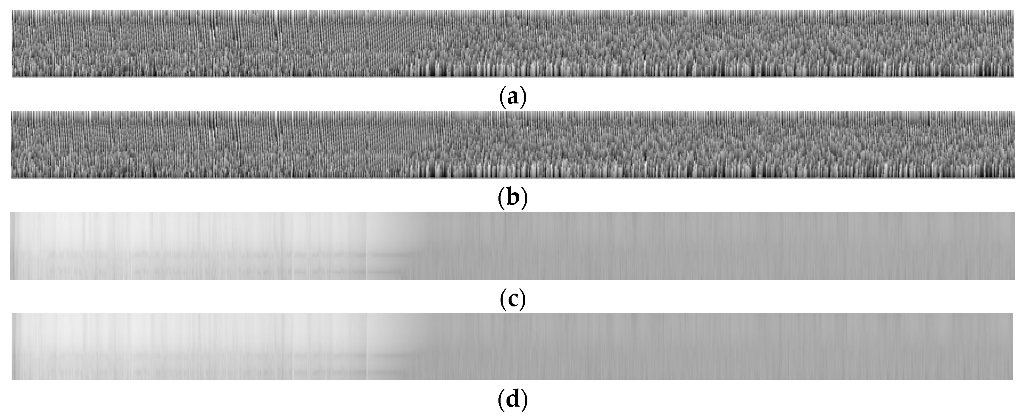
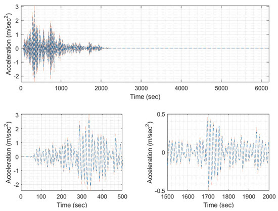
Figure A16.
Predicted EQ response time history (blue) compared to the target one (orange) of signal 6002 (model #711, EQ #8).
Figure A16.
Predicted EQ response time history (blue) compared to the target one (orange) of signal 6002 (model #711, EQ #8).

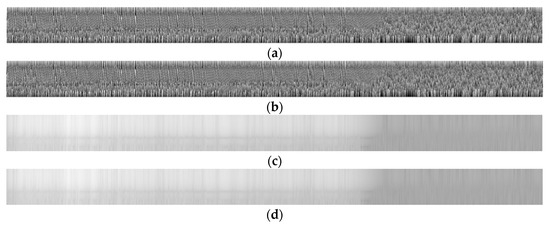
Figure A17.
A sample of input/output set of images for training, with (a) EQ response phase target (signal 6003), (b) EQ response phase predicted (signal 6003), (c) EQ response magnitude target (signal 6003), and (d) EQ response magnitude predicted (signal 6003).
Figure A17.
A sample of input/output set of images for training, with (a) EQ response phase target (signal 6003), (b) EQ response phase predicted (signal 6003), (c) EQ response magnitude target (signal 6003), and (d) EQ response magnitude predicted (signal 6003).
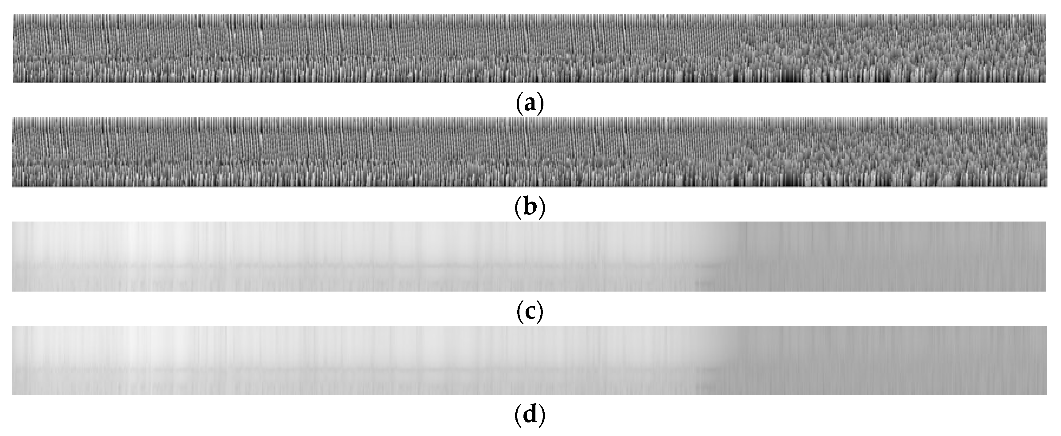
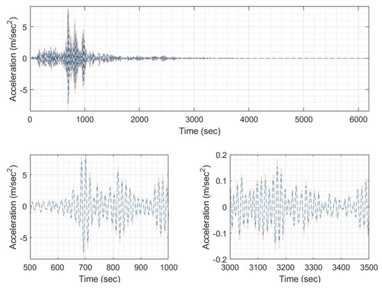
Figure A18.
Predicted EQ response time history (blue) compared to the target one (orange) of signal 6003 (model #711, EQ #9).
Figure A18.
Predicted EQ response time history (blue) compared to the target one (orange) of signal 6003 (model #711, EQ #9).
References
- Vincent, P.; Larochelle, H.; Lajoie, I.; Bengio, Y.; Manzagol, P.A.; Bottou, L. Stacked denoising autoencoders: Learning useful representations in a deep network with a local denoising criterion. J. Mach. Learn. Res. 2010, 11, 3371–3408. [Google Scholar]
- Rumelhart, D.E.; Hinton, G.E.; Williams, R.J. Learning representations by back-propagating errors. Nature 1986, 323, 533–536. [Google Scholar] [CrossRef]
- LeCun, Y.; Boser, B.; Denker, J.S.; Henderson, D.; Howard, R.E.; Hubbard, W.; Jackel, L.D. Backpropagation Applied to Handwritten Zip Code Recognition. Neural Comput. 1989, 1, 541–551. [Google Scholar] [CrossRef]
- LeCun, Y.; Bengio, Y. Convolutional networks for images, speech, and time series. In The Handbook of Brain Theory and Neural Networks; MIT Press: Cambridge, MA, USA, 1995; Volume 3361. [Google Scholar]
- LeCun, Y.; Bottou, L.; Bengio, Y.; Haffner, P. Gradient-based learning applied to document recognition. Proc. IEEE 1998, 86, 2278–2324. [Google Scholar] [CrossRef]
- LeCun, Y.; Kavukcuoglu, K.; Farabet, C. Convolutional networks and applications in vision. In Circuits and Systems (ISCAS), Proceedings of 2010 International Symposium on Circuits and Systems, Paris, France, 13–18 June 2010; IEEE: New York, NY, USA; pp. 253–256.
- Hopfield, J.J. Neural networks and physical systems with emergent collective computational abilities. Proc. Natl. Acad. Sci. USA 1982, 79, 2554–2558. [Google Scholar] [CrossRef] [PubMed]
- Hochreiter, S.; Schmidhuber, J. Long short-term memory. Neural Comput. 1997, 9, 1735–1780. [Google Scholar] [CrossRef] [PubMed]
- Hinton, G.E.; Osindero, S.; Teh, Y.W. A fast learning algorithm for deep belief nets. Neural Comput. 2006, 18, 1527–1554. [Google Scholar] [CrossRef] [PubMed]
- Vaswani, A.; Shazeer, N.; Parmar, N.; Uszkoreit, J.; Jones, L.; Gomez, A.N.; Kaiser, L.; Polosukhin, I. Attention is all you need. In Proceedings of the Advances in Neural Information Processing Systems, Long Beach, CA, USA, 4–9 December 2017; pp. 5998–6008. [Google Scholar]
- Ruggieri, S.; Cardellicchio, A.; Leggieri, V.; Uva, G. Machine-learning based vulnerability analysis of existing buildings. Autom. Constr. 2021, 132, 103936. [Google Scholar] [CrossRef]
- Cardellicchio, A.; Ruggieri, S.; Nettis, A.; Renò, V.; Uva, G. Physical interpretation of machine learning-based recognition of defects for the risk management of existing bridge heritage. Eng. Fail. Anal. 2023, 149, 107237. [Google Scholar] [CrossRef]
- OASP. First Level Pre-Quake Rapid Visual Inspection (RVI). 2023. Available online: https://oasp.gr/proseismikos-eleghos/proseismikos-eleghos-ktirion-dimosias-kai-koinofeloys-hrisis (accessed on 6 March 2023).
- Applied Technology Council and the Consortium of Universities for Research in Earthquake Engineering (ATC/CUREE). FEMA P-58, Seismic Performance Assessment of Buildings: Methodology and Implementation; Federal Emergency Management Agency: Washington, DC, USA, 2012. [Google Scholar]
- OpenSees. Pacific Earthquake Engineering Research Center, University of California, Berkeley. 2023. Available online: https://opensees.berkeley.edu/ (accessed on 19 March 2023).
- OpenQuake. Global Earthquake Model Foundation. 2023. Available online: https://www.globalquakemodel.org/openquake/ (accessed on 19 March 2023).
- Pagani, M.; Weatherill, G.; Monelli, D. OpenQuake: A modular open-source software for earthquake hazard and risk analysis. Seismol. Res. Lett. 2014, 85, 692–702. [Google Scholar] [CrossRef]
- Malekloo, A.; Ozer, E.; AlHamaydeh, M.; Girolami, M. Machine learning and structural health monitoring overview with emerging technology and high-dimensional data source highlights. Struct. Health Monit. 2022, 21, 1906–1955. [Google Scholar] [CrossRef]
- Azimi, M.; Eslamlou, A.D.; Pekcan, G. Data-Driven Structural Health Monitoring and Damage Detection through Deep Learning: State-of-the-Art Review. Sensors 2020, 20, 2778. [Google Scholar] [CrossRef] [PubMed]
- Won, J.; Shin, J. Machine learning-based approach for seismic damage prediction method of building structures considering soil-structure interaction. Sustainability 2021, 13, 4334. [Google Scholar] [CrossRef]
- Rachedi, M.; Matallah, M.; Kotronis, P. Seismic behavior & risk assessment of an existing bridge considering soil-structure interaction using artificial neural networks. Eng. Struct. 2021, 232, 111800. [Google Scholar]
- Yu, Y.; Wang, C.; Gu, X.; Li, J. A novel deep learning-based method for damage identification of smart building structures. Struct. Health Monit. 2019, 18, 143–163. [Google Scholar] [CrossRef]
- Oh, B.K.; Park, Y.; Park, H.S. Seismic response prediction method for building structures using convolutional neural network. Struct. Control. Health Monit. 2020, 27, e2519. [Google Scholar] [CrossRef]
- ADINA R&D Inc.: ADINA. Version: 9.2.1. Available online: http://www.adina.com (accessed on 25 May 2023).
- Kocak, S.; Mengi, Y. A simple soil–structure interaction model. Appl. Math. Model. 2000, 24, 607–635. [Google Scholar] [CrossRef]
- Federal Emergency Management Agency. FEMA: Hazus—MH 2.1: Technical Manual; Department of Homeland Security, Federal Emergency Management Agency, Mitigation Division: Washington, DC, USA, 2013. [Google Scholar]
- Welch, P. The use of fast Fourier transform for the estimation of power spectra: A method based on time averaging over short, modified periodograms. IEEE Trans. Audio Electroacoust. 1967, 15, 70–73. [Google Scholar] [CrossRef]
- Rabiner, L.I.; Gold, B. Theory and Application of Digital Signal Processing; Prentice-Hall: Saddle River, NJ, USA, 1975. [Google Scholar]
- Kay, S. Spectral Estimation; Prentice-Hall, Inc.: Saddle River, NJ, USA, 1987; pp. 58–122. [Google Scholar]


Disclaimer/Publisher’s Note: The statements, opinions and data contained in all publications are solely those of the individual author(s) and contributor(s) and not of MDPI and/or the editor(s). MDPI and/or the editor(s) disclaim responsibility for any injury to people or property resulting from any ideas, methods, instructions or products referred to in the content. |
© 2023 by the authors. Licensee MDPI, Basel, Switzerland. This article is an open access article distributed under the terms and conditions of the Creative Commons Attribution (CC BY) license (https://creativecommons.org/licenses/by/4.0/).