

Experimental and Numerical Study of the Thermal Properties of Dry Green Swales to Be Used as Part of Geothermal Energy Systems


Abstract
:Featured Application
Abstract
1. Introduction
- Characterization of the thermal properties of the materials used in the green swale cross-sections.
- Identification and determination of the effect of the use of non-conventional materials such as expanded clay and construction and demolition waste (CDW) on the thermal behavior of a SuDS.
- Laboratory determination of the key thermal parameters of the different layers of the green swale sections by means of standardized tests, and analyzing their thermal behavior and their implications in a system combined with surface geothermal energy in dry and wet operating conditions.
- Validation of the results obtained in the laboratory tests by means of steady-state numerical simulations, Design of Experiments (DOE), and the use of Multi-Objective Genetic Algorithms (MOGAs).
- Simulation of the behavior of green swales in real operating conditions, using transient state numerical models.
2. Materials and Methods
2.1. Materials
- Material 1: Vegetable land (topsoil) with an apparent density of 1400 kg/m3. This material was used as the surface layer in all the studied models.
- Material 2: Limestone aggregate with a particle size of 0/32 mm, apparent density of 2690 kg/m3, and porosity of 35%.
- Material 3: Expanded clay with a particle size of 10/20 mm, apparent density of 275 kg/m3, and porosity of 34%. Expanded clay, due to its industrial manufacturing process, has a higher porosity, a lower density, and a vitrified surface [45].
- Material 4: Mixed CDW (combined recycled aggregate of mixed origin) 0/32, following the specifications the EN 13242:2Q02 + A1:2007 standard [46]. It has a particle density of 2.5 + 0.2 mg/m3 and a water absorption rate of less than 7%.
- Material 5: Infiltration cells. A modular tank system that provides up to 90% void space and has a thickness of 52 mm was constructed through the use of the Atlantis Flo-Cell® infiltration cell. The cells allowed efficient water drainage, while retaining an optimal moisture level for the overlying vegetative layers. This material was used as the drainage layer in all the models.
2.2. Materials Characterization
- Ambient conditions, with the materials tested under laboratory-controlled temperature and relative humidity (RH): T = 18.5 ± 0.5 °C and RH = 80%.
- Wet conditions, where the materials were tested under saturated conditions. In the case of the expanded clay and topsoil layers, water was added gradually until a soft consistent paste was formed. For the limestone aggregate specimens, they were immersed in a container with water at a constant temperature of 22.4 ± 0.5 °C for 168.0 ± 0.5 h until they reached full saturation.
2.3. Experimental Set-Up
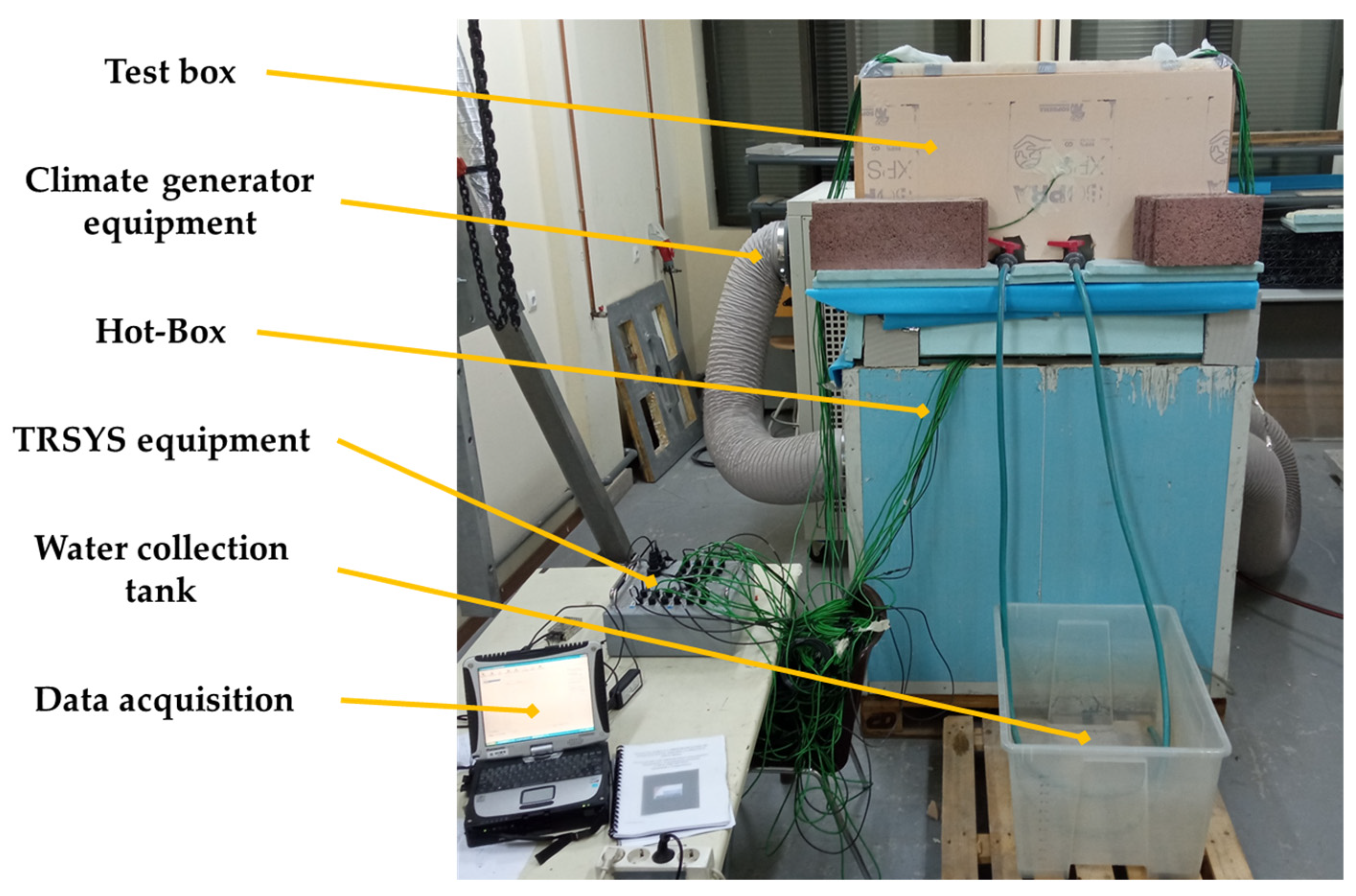
- Climatic generator: This equipment allows for precise control of relative humidity and temperature values in an enclosed environment, ensuing constant cold, heat, and humidity.
- Calibrated hot-box: A fully insulated 1 m3 capacity hot-box is connected to the climatic generator equipment (see Figure 3). The calibrated hot-box is used to create an environment under controlled temperature and humidity conditions for each test. The above-mentioned equipment operates as indicated in the UNE-EN ISO 8990:1997 [51] and ASTM C1363:19 standards [52].
- Test-box: This is the container in which the tested green swale cross-sections were introduced and set up according to the experimental procedure. It has interior dimensions of 608 × 408 mm2 at the bottom. The test-box is installed over the hot-box (see Figure 3) so that the heat flux passes perpendicularly through the surface of the studied green swale cross-section from its bottom layer. The test-box is thermally insulated from the outside with 20 cm of extruded polystyrene (0.033 ± 0.003 W/mK) in order to minimize lateral heat losses.
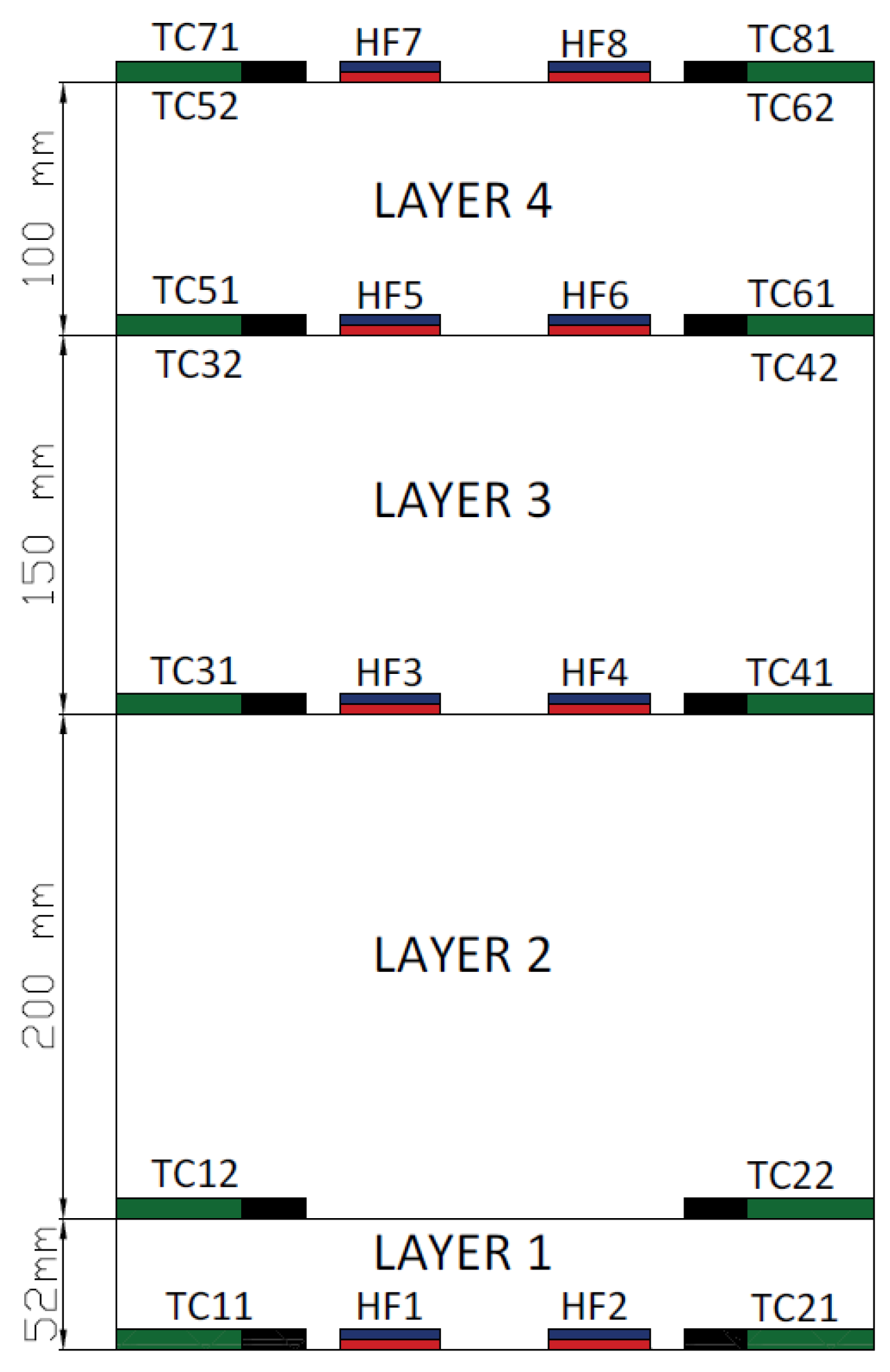
- Temperature and heat flux sensors: Fourteen type K thermocouples (TCxy) were installed according to the distribution shown in Figure 4. Additionally, two extra thermocouples were used to determine the heat loss through the walls of the Test-box. Eight thermal flux sensors (HFx) Hukseflux HFP01 were employed, and they were installed at the interfaces of all the layers (see Figure 4). The technical specifications of the thermal flux sensors are as follows: sensitivity, 60 × 10−6 V/(W/m2); thermal resistance of the sensor, 71 × 10−4 K/(W/m2); nominal operating temperature range, −30 to +70 °C; and measurement range, −2000 to +2000 W/m2.
- TRSYS equipment: This system was used to acquire data from the aforementioned sensors, and it was programmed to collect information in 10 min interval. It also allows for data storage and transmission for further analyses.
2.4. Calculation of the Thermal Conductivity: Physical Principles
2.5. Experimental Methodology
2.6. Numerical Models
2.6.1. Steady-State Thermal Model
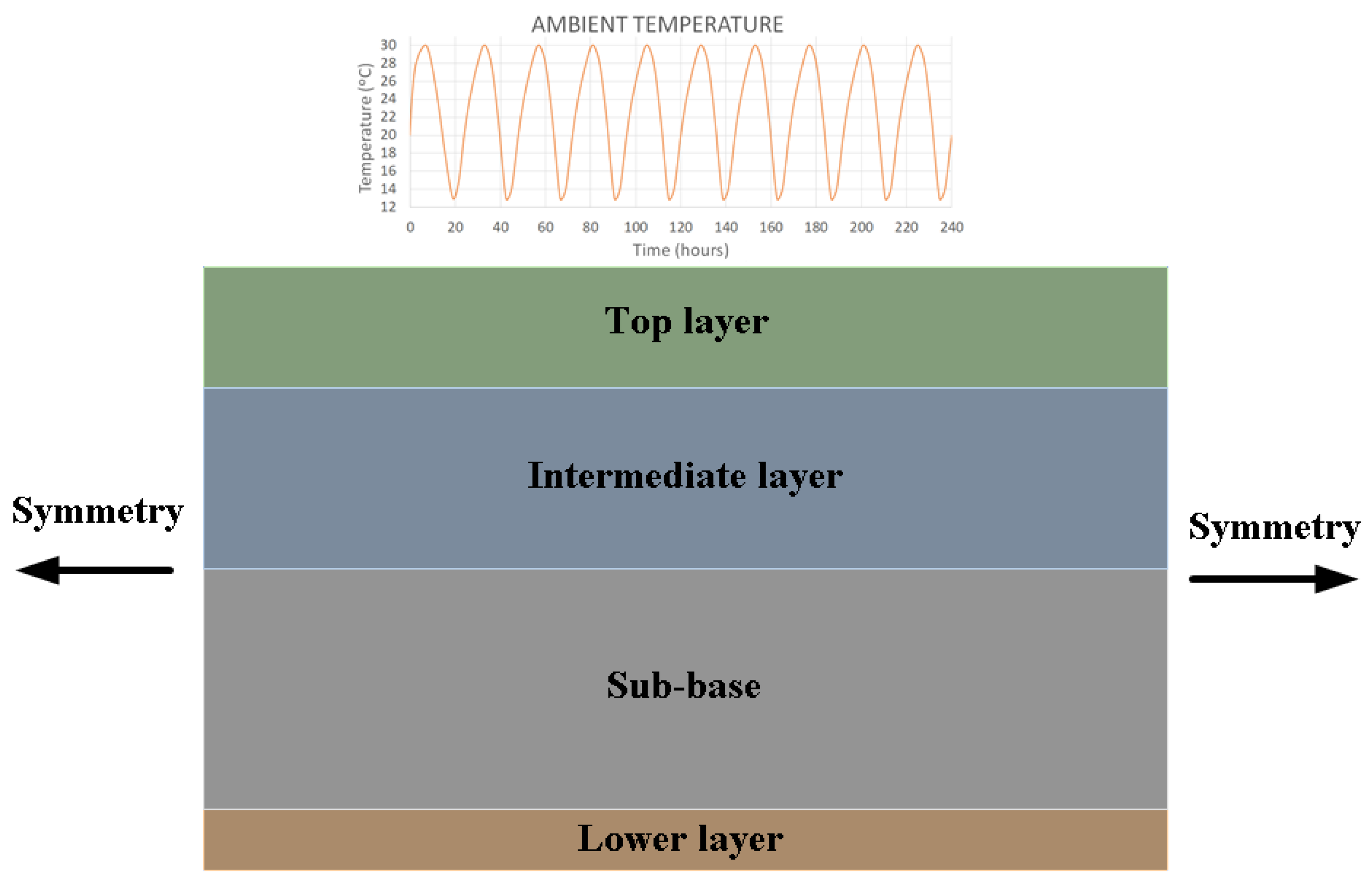
2.6.2. Transient Thermal Model
3. Results and Discussion
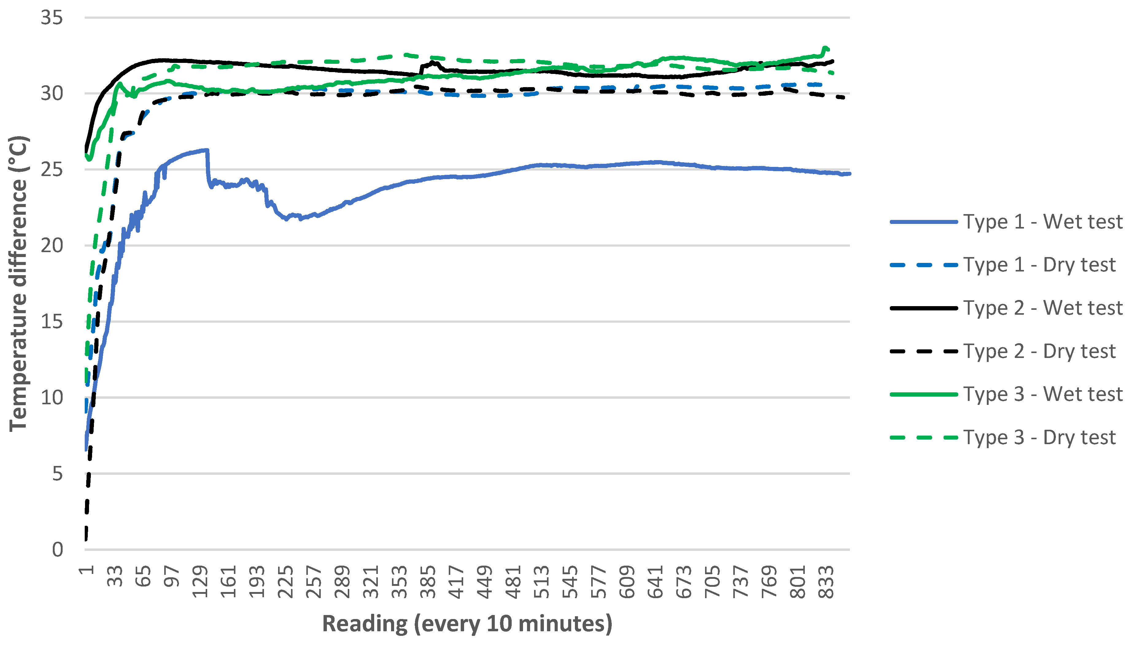
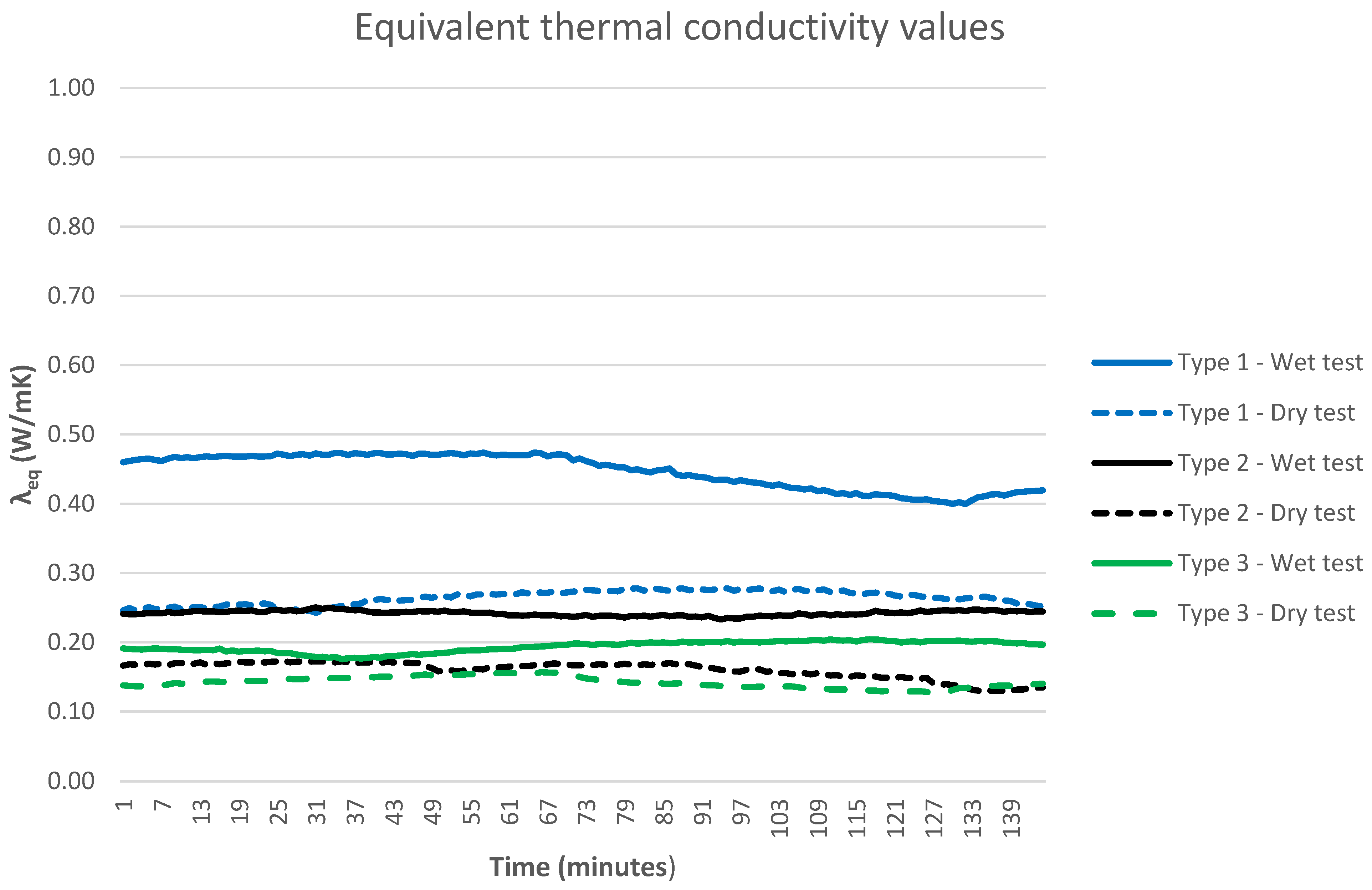
3.1. Experimental Results
3.2. Numerical Results
3.2.1. Mesh Sensitivity Analysis
3.2.2. Steady-State Thermal Model Results
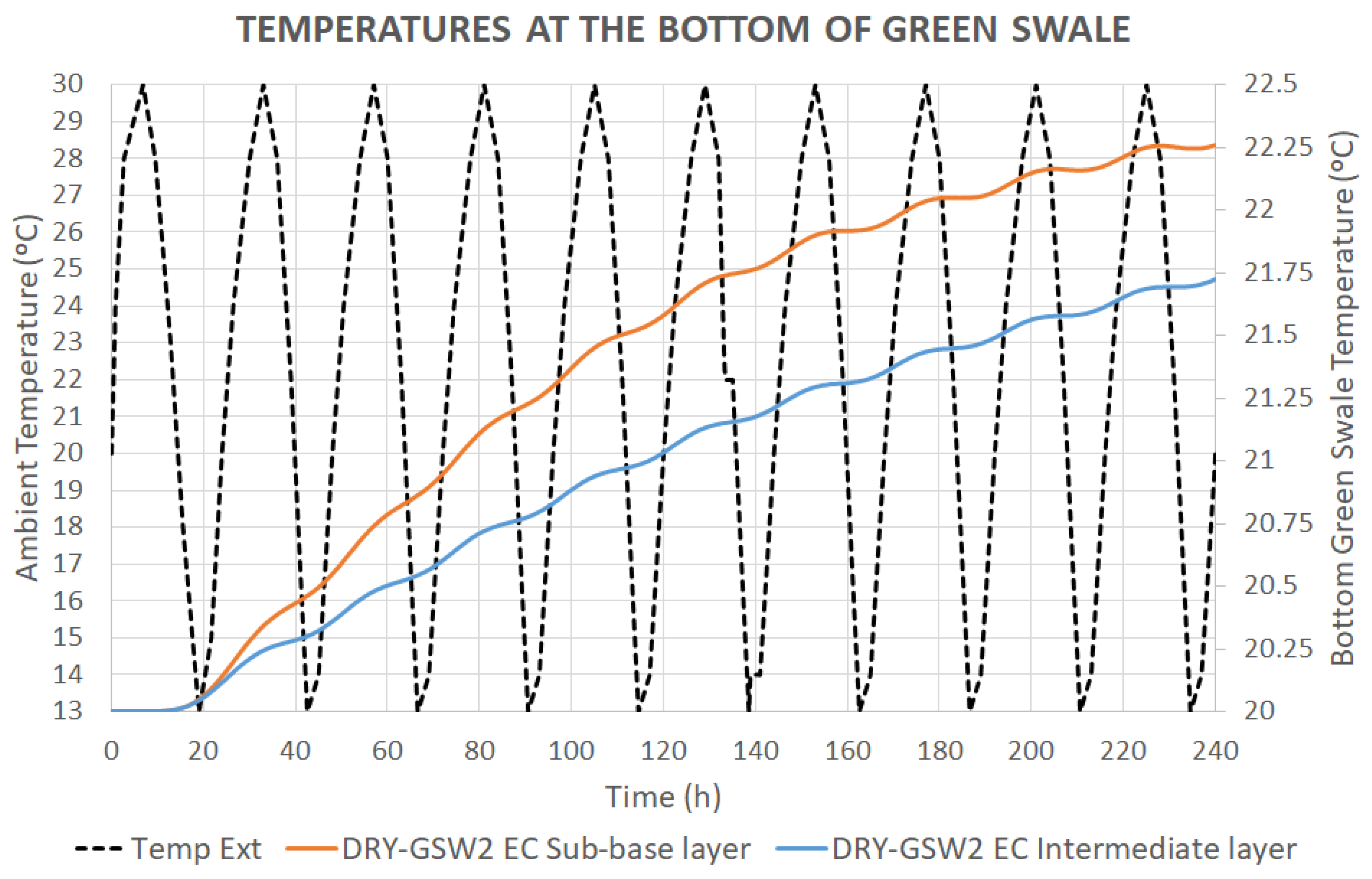
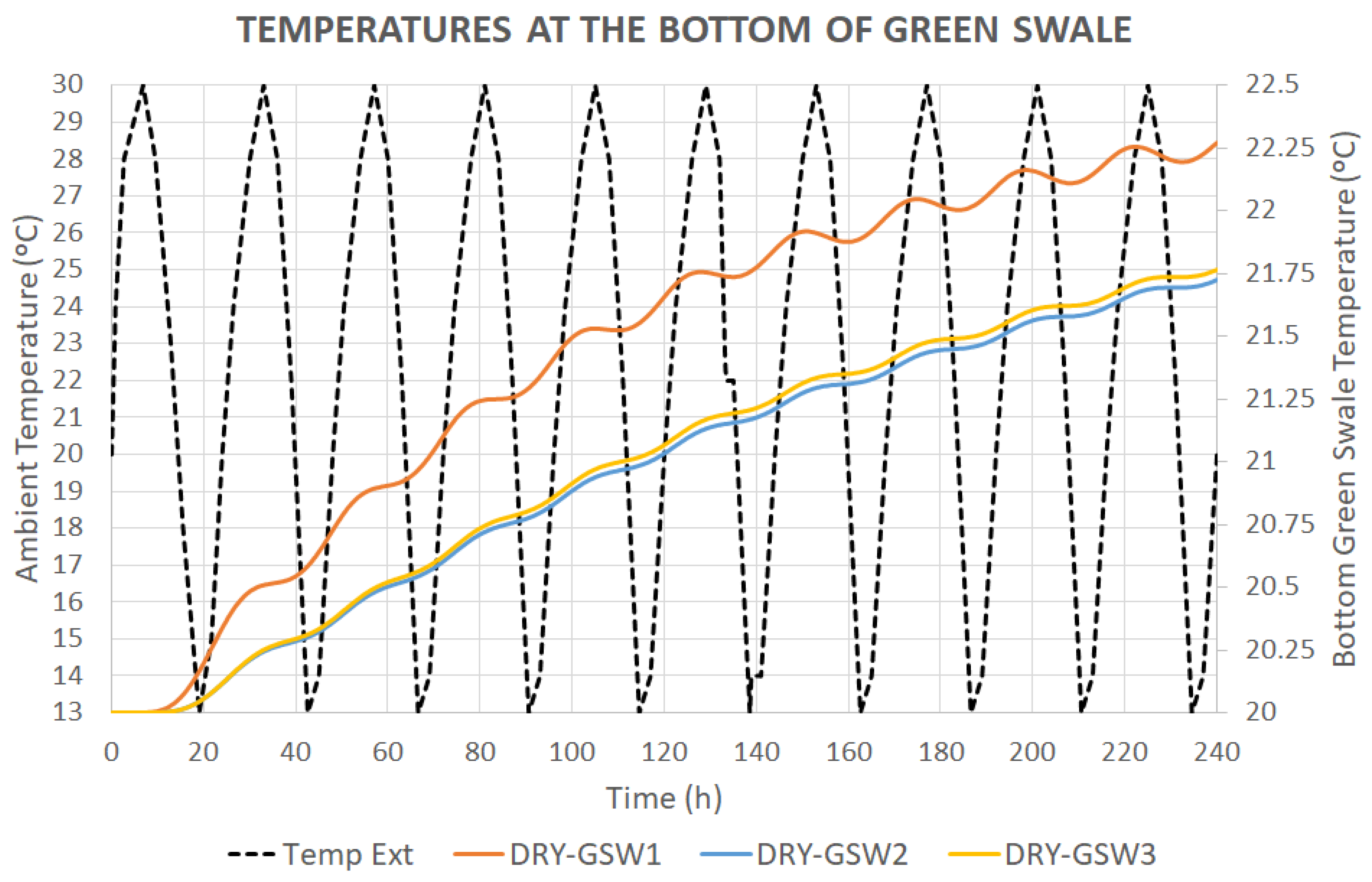
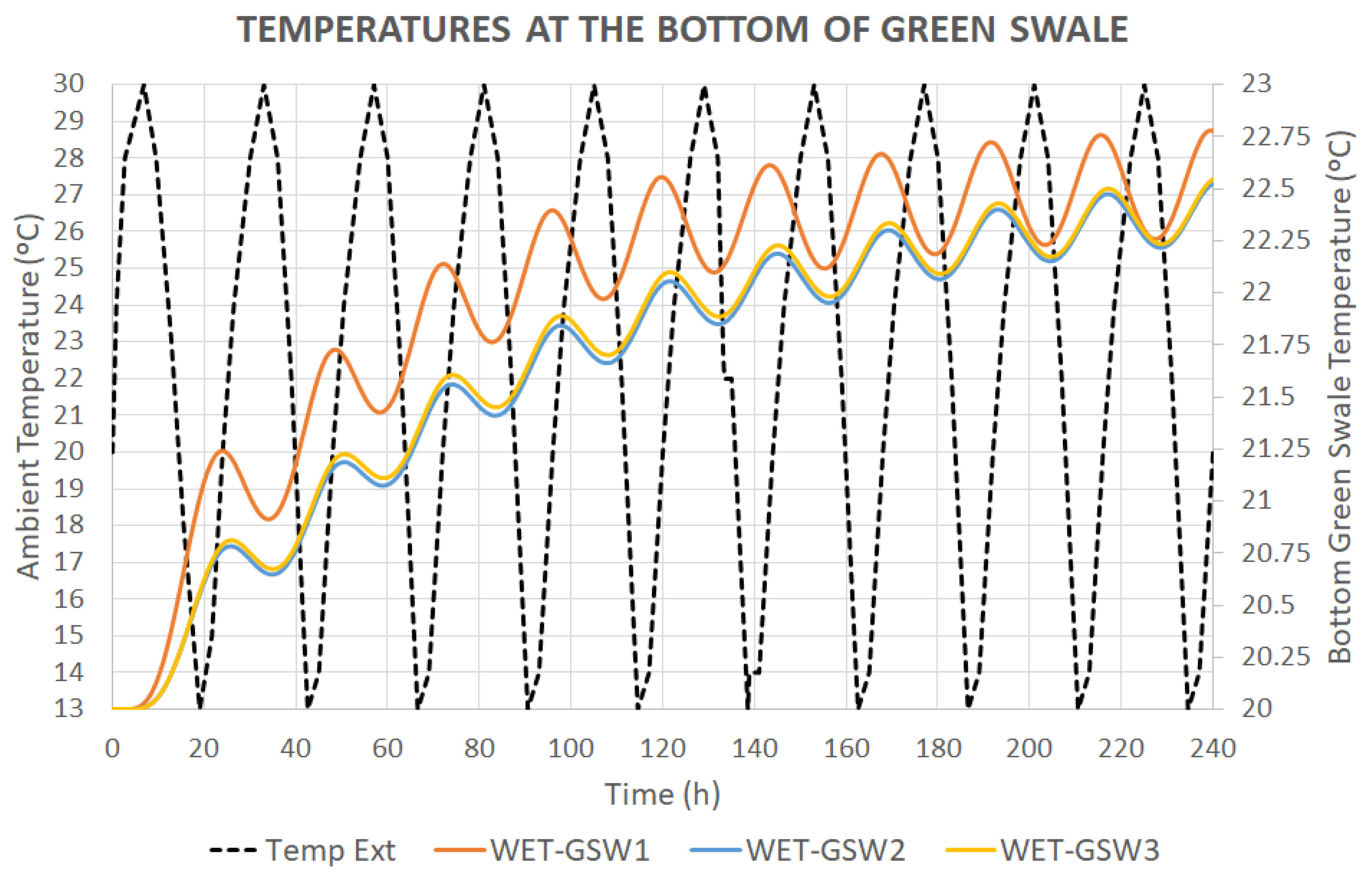
3.2.3. Transient Thermal Model Results
4. Conclusions and Future Research Directions
Author Contributions
Funding
Institutional Review Board Statement
Informed Consent Statement
Data Availability Statement
Acknowledgments
Conflicts of Interest
Nomenclature
| Acronyms | |
| CDW | Construction and demolition waste |
| DOE | Design of Experiments |
| EU | European Union |
| FEM | Finite Element Analysis |
| GHE | Geothermal Heat Exchanger |
| GI | Green infrastructure |
| GSHP | Ground-source heat pump |
| GHP | Guarded-hot-plate |
| LID | Low impact development |
| MIT | Massachusetts Institute of Technology |
| MTPS | Modified transient plane source |
| MOGA | Multi-Objective Genetic Algorithm |
| NBS | Nature-based solutions |
| PPS | Permeable Pavement Systems |
| SCM | Stormwater constructed measures |
| SDGs | Sustainable Development Goals |
| SGS | Shallow geothermal system |
| SuDS | Sustainable Drainage System |
| TRT | Thermal Response Test |
| THW | Transient-hot-wire |
| UN | United Nations |
| Symbols | |
| Thermal transmittance () | |
| Temperature differential () | |
| Thermal gradient between the heat source and the heat sink (K/m) | |
| Average heat flux () | |
| RH | Relative humidity (%) |
| S | Sample standard deviation |
| Total thickness of the green swale model () | |
| Thermal conductivity in the x direction () | |
| Equivalent thermal conductivity () | |
| Heat flux per unit area in the interlayer () | |
| kTCC | Thermal contact conductance coefficient () |
| Tc,T; Tc,C | Temperatures of the contacts points () |
| Density of the material (kg/m3) | |
| Ef | Thermal effusivity (Ws1/2/m2K) |
| Cp | Specific heat (J/kgK) |
References
- International Energy Agency (IEA). Net Zero by 2050—A Roadmap for the Global Energy Sector; International Energy Agency: Paris, France, 2021. [Google Scholar]
- Tester, J.W. The Future of Geothermal Energy: Impact of Enhanced Geothermal Systems (EGS) on the United States in the 21st Century; Massachusetts Institute of Technology: Cambridge, MA, USA, 2006. [Google Scholar]
- United Nations (UN). Transforming Our World: The 2030 Agenda for Sustainable Development; United Nations: New York, NY, USA, 2015. [Google Scholar]
- Council of the European Union Council Conclusions on Climate and Energy Diplomacy. Bolstering EU Climate and Energy Diplomacy in a Critical Decade; European Union: Brussels, Belgium, 2023. [Google Scholar]
- Ervine, C. Directive 2004/39/Ec of the European Parliament and of the Council of 21 April 2004. In Core Statutes on Company Law; Macmillan Education: London, UK, 2015; pp. 757–759. ISBN 978-1-137-54506-0. [Google Scholar]
- U.S. Department of Energy. GeoVision: Harnessing the Heat Beneath Our Feet; U.S. Department of Energy: Washington, DC, USA, 2019.
- Espanya; Ministerio de Industria, Comercio y Turismo; Espanya; Ministerio de Ciencia e Innovación; Instituto para la Diversificación y Ahorro de la Energía; Instituto Geológico y Minero de España. Manual de Geotermia; IDAE: Madrid, Spain, 2008; ISBN 978-84-96680-35-7. [Google Scholar]
- Instituto para la Diversificación y Ahorro de la Energía (IDAE). Guía Técnica de Diseño de Sistemas de Intercambio Geotérmico de Circuito Cerrado; Instituto para la Diversificación y Ahorro de la Energía (IDAE): Madrid, Spain, 2012. [Google Scholar]
- Assad, M.E.H.; Bani-Hani, E.; Khalil, M. Performance of geothermal power plants (single, dual, and binary) to compensate for LHC-CERN power consumption: Comparative study. Geotherm. Energy 2017, 5, 17. [Google Scholar] [CrossRef]
- Urresta, E.; Moya, M.; Campana, C.; Cruz, C. Ground Thermal Conductivity Estimation Using the Thermal Response Test with a Horizontal Ground Heat Exchanger. Geothermics 2021, 96, 102213. [Google Scholar] [CrossRef]
- Chomać-Pierzecka, E.; Sobczak, A.; Soboń, D. The Potential and Development of the Geothermal Energy Market in Poland and the Baltic States—Selected Aspects. Energies 2022, 15, 4142. [Google Scholar] [CrossRef]
- Trillo, G.L.; Angulo, V.R. Guía de La Energía Geotérmica; Dirección General de Industria, Energía y Minas: Madrid, Spain, 2008. [Google Scholar]
- Sañudo-Fontaneda, L.A.; Roces-García, J.; Coupe, S.J.; Barrios-Crespo, E.; Rey-Mahía, C.; Álvarez-Rabanal, F.P.; Lashford, C. Descriptive Analysis of the Performance of a Vegetated Swale through Long-Term Hydrological Monitoring: A Case Study from Coventry, UK. Water 2020, 12, 2781. [Google Scholar] [CrossRef]
- Congedo, P.M.; Colangelo, G.; Starace, G. CFD Simulations of Horizontal Ground Heat Exchangers: A Comparison among Different Configurations. Appl. Therm. Eng. 2012, 33–34, 24–32. [Google Scholar] [CrossRef]
- Di Sipio, E.; Bertermann, D. Factors Influencing the Thermal Efficiency of Horizontal Ground Heat Exchangers. Energies 2017, 10, 1897. [Google Scholar] [CrossRef]
- Rey-Mahia, C.; Álvarez-Rabanal, F.P.; Coupe, S.J.; Sañudo Fontaneda, L.Á. The Role of Geothermal Heat Pump Systems in the Water–Energy Nexus. In Geothermal Heat Pump Systems; Green Energy and Technology; Springer International Publishing: Cham, Switzerland, 2023; ISBN 978-3-031-24523-7. [Google Scholar]
- De Oliveira, G.C.; Bertone, E.; Stewart, R.A. Challenges, Opportunities, and Strategies for Undertaking Integrated Precinct-Scale Energy–Water System Planning. Renew. Sustain. Energy Rev. 2022, 161, 112297. [Google Scholar] [CrossRef]
- Faraj-Lloyd, A.; Charlesworth, S.M.; Coupe, S.J. Sustainable Drainage Systems and Energy: Generation and Reduction. In Sustainable Surface Water Management; Charlesworth, S.M., Booth, C.A., Eds.; Wiley: Hoboken, NJ, USA, 2017; pp. 177–192. ISBN 978-1-118-89770-6. [Google Scholar]
- Chan, F.K.S.; Griffiths, J.A.; Higgitt, D.; Xu, S.; Zhu, F.; Tang, Y.-T.; Xu, Y.; Thorne, C.R. “Sponge City” in China—A Breakthrough of Planning and Flood Risk Management in the Urban Context. Land Use Policy 2018, 76, 772–778. [Google Scholar] [CrossRef]
- Ayuntamiento de Madrid. Guía Básica de Diseño de Sistemas de Gestión Sostenible de Aguas Pluviales En Zonas Verdes y Otros Espacios Libres; Dirección General de Gestión del Agua y Zonas Verdes: Madrid, Spain, 2018. [Google Scholar]
- Fletcher, T.D.; Shuster, W.; Hunt, W.F.; Ashley, R.; Butler, D.; Arthur, S.; Trowsdale, S.; Barraud, S.; Semadeni-Davies, A.; Bertrand-Krajewski, J.-L.; et al. SUDS, LID, BMPs, WSUD and More—The Evolution and Application of Terminology Surrounding Urban Drainage. Urban Water J. 2015, 12, 525–542. [Google Scholar] [CrossRef]
- Sañudo-Fontaneda, L.A.; Rodriguez-Hernandez, J.; Castro-Fresno, D. Diseño y Construcción de Sistemas Urbanos de Drenaje Sostenible (SUDS); School of Civil Engineering of the Universidad de Cantabria: Santander, Spain, 2012. [Google Scholar]
- North Carolina Department of Environmental Quality. Stormwater Design Maintenance; North Carolina Department of Environmental Quality: Raleigh, NC, USA, 2017.
- Charlesworth, S.M.; Faraj-Llyod, A.S.; Coupe, S.J. Renewable Energy Combined with Sustainable Drainage: Ground Source Heat and Pervious Paving. Renew. Sustain. Energy Rev. 2017, 68, 912–919. [Google Scholar] [CrossRef]
- Jato-Espino, D.; Sañudo-Fontaneda, L.A.; Andrés-Valeri, V.C. Green Infrastructure: Cost-Effective Nature-Based Solutions for Safeguarding the Environment and Protecting Human Health and Well-Being. In Handbook of Environmental Materials Management; Hussain, C.M., Ed.; Springer International Publishing: Cham, Switzerland, 2018; pp. 1–27. ISBN 978-3-319-58538-3. [Google Scholar]
- del-Castillo-García, G.; Borinaga-Treviño, R.; Sañudo-Fontaneda, L.A.; Pascual-Muñoz, P. Influence of Pervious Pavement Systems on Heat Dissipation from a Horizontal Geothermal System. Eur. J. Environ. Civ. Eng. 2013, 17, 956–967. [Google Scholar] [CrossRef]
- Tota-Maharaj, K.; Scholz, M.; Ahmed, T.; French, C.; Pagaling, E. The Synergy of Permeable Pavements and Geothermal Heat Pumps for Stormwater Treatment and Reuse. Environ. Technol. 2010, 31, 1517–1531. [Google Scholar] [CrossRef]
- Tota-Maharaj, K.; Paul, P. Sustainable Approaches for Stormwater Quality Improvements with Experimental Geothermal Paving Systems. Sustainability 2015, 7, 1388–1410. [Google Scholar] [CrossRef]
- Rey-Mahía, C.; Sañudo-Fontaneda, L.A.; Andrés-Valeri, V.C.; Álvarez-Rabanal, F.P.; Coupe, S.J.; Roces-García, J. Evaluating the Thermal Performance of Wet Swales Housing Ground Source Heat Pump Elements through Laboratory Modelling. Sustainability 2019, 11, 3118. [Google Scholar] [CrossRef]
- Mayor’s Office of Transportatios and Utilities, City of Philadelphia. City of Philadelphia Green Streets Desing Manual; Mayor’s Office of Transportatios and Utilities, City of Philadelphia: Philadelphia, PA, USA, 2014.
- Woods-Ballard, B.; Wilson, S.; Udale-Clarke, H.; Illman, S.; Scott, T.; Ashley, R.; Kellagher, R. The SuDS Manual; CIRIA: London, UK, 2015; ISBN 978-0-86017-760-9. [Google Scholar]
- Florides, G.; Kalogirou, S. Ground Heat Exchangers—A Review of Systems, Models and Applications. Renew. Energy 2007, 32, 2461–2478. [Google Scholar] [CrossRef]
- Aresti, L.; Christodoulides, P.; Florides, G. A Review of the Design Aspects of Ground Heat Exchangers. Renew. Sustain. Energy Rev. 2018, 92, 757–773. [Google Scholar] [CrossRef]
- Gil, A.G. Geotermia Somera: Fundamentos Teóricos y Aplicación; Instituto Geológico y Minero de España: Madrid, Spain, 2020; ISBN 978-84-9138-105-1. [Google Scholar]
- Hou, G.; Taherian, H.; Song, Y.; Jiang, W.; Chen, D. A Systematic Review on Optimal Analysis of Horizontal Heat Exchangers in Ground Source Heat Pump Systems. Renew. Sustain. Energy Rev. 2022, 154, 111830. [Google Scholar] [CrossRef]
- Rottmann, M.; Beikircher, T.; Ebert, H.-P. Thermal Conductivity of Evacuated Expanded Perlite Measured with Guarded-Hot-Plate and Transient-Hot-Wire Method at Temperatures between 295 K and 1073 K. Int. J. Therm. Sci. 2020, 152, 106338. [Google Scholar] [CrossRef]
- Kim, D.; Oh, S. Measurement and Comparison of Thermal Conductivity of Porous Materials Using Box, Dual-Needle, and Single-Needle Probe Methods-A Case Study. Int. Commun. Heat Mass Transf. 2020, 118, 104815. [Google Scholar] [CrossRef]
- Poulsen, S.E.; Andersen, T.R.; Tordrup, K.W. Full-Scale Demonstration of Combined Ground Source Heating and Sustainable Urban Drainage in Roadbeds. Energies 2022, 15, 4505. [Google Scholar] [CrossRef]
- Andersen, T.R.; Poulsen, S.E.; Tordrup, K.W. The Climate Road—A Multifunctional Full-Scale Demonstration Road That Prevents Flooding and Produces Green Energy. Water 2022, 14, 666. [Google Scholar] [CrossRef]
- Rey-Mahía, C.; Álvarez-Rabanal, F.P.; Sañudo-Fontaneda, L.A.; Hidalgo-Tostado, M.; Menéndez Suárez-Inclán, A. An Experimental and Numerical Approach to Multifunctional Urban Surfaces through Blue Roofs. Sustainability 2022, 14, 1815. [Google Scholar] [CrossRef]
- Borinaga-Treviño, R.; Pascual-Muñoz, P.; Castro-Fresno, D.; Del Coz-Díaz, J.J. Study of Different Grouting Materials Used in Vertical Geothermal Closed-Loop Heat Exchangers. Appl. Therm. Eng. 2013, 50, 159–167. [Google Scholar] [CrossRef]
- Di Sipio, E.; Chiesa, S.; Destro, E.; Galgaro, A.; Giaretta, A.; Gola, G.; Manzella, A. Rock Thermal Conductivity as Key Parameter for Geothermal Numerical Models. Energy Procedia 2013, 40, 87–94. [Google Scholar] [CrossRef]
- Del Coz Díaz, J.J.; Álvarez Rabanal, F.P.; García Nieto, P.J.; Domínguez Hernández, J.; Rodríguez Soria, B.; Pérez-Bella, J.M. Hygrothermal Properties of Lightweight Concrete: Experiments and Numerical Fitting Study. Constr. Build. Mater. 2013, 40, 543–555. [Google Scholar] [CrossRef]
- Fuente-García, L.; Perales-Momparler, S.; Rico-Cortés, M.; Andrés-Doménech, I.; Marco-Segura, J.B. Guía Básica para el Diseño de Sistemas Urbanos de Drenaje Sostenible en la Ciudad de València; Ajuntament de València: Valencia, Spain, 2021; ISBN 978-84-9089-386-9. [Google Scholar]
- Rashad, A.M. Lightweight Expanded Clay Aggregate as a Building Material—An Overview. Constr. Build. Mater. 2018, 170, 757–775. [Google Scholar] [CrossRef]
- UNE-EN 13242:2003+A1:2008; Aggregates for Unbound and Hydraulically Bound Materials for Use in Civil Engineering Work and Road Construction. European Standards: Plzen, Czech Republic, 2008.
- UNE-EN 933-1:2012; Test for Geometrical Properties of Aggregates. Part 1: Determination of Particle Size Distribution. Sieving Method. European Standards: Plzen, Czech Republic, 2012.
- UNE-EN ISO 22007-2:2023; Plastics. Determination of Thermal Conductivity and Thermal Diffusivity. Part 2: Transient Plane Heat Source (Hot Disc) Method. European Standards: Plzen, Czech Republic, 2023.
- ASTM D7984:21; Standard Test Method for Measurement of Thermal Effusivity of Fabrics Using a Modified Transient Plane Source (MTPS) Instrument. ASTM International: West Conshohocken, PA, USA, 2021.
- UNE-EN 1097-6:2014; Tests for Mechanical and Physical Properties of Aggregates—Part 6: Determination of Particle Density and Water Absorption. European Standards: Plzen, Czech Republic, 2014.
- UNE-EN ISO 8990:1997; Thermal Insulation. Determination of Steady-State Thermal Transmission Properties. Calibrated and Guarded Hot Box (ISO 8990:1994). European Standards: Plzen, Czech Republic, 1997.
- ASTM C1363:19; Standard Test Method for Thermal Performance of Building Materials and Envelope Assemblies by Means of a Hot Box Apparatus. ASTM International: West Conshohocken, PA, USA, 2019.
- Cengel, Y. Transferencia de Calor y Masa. Fundamentos y Aplicaciones; McGraw-Hill Education: Columbus, OH, USA, 2020; ISBN 978-607-15-1461-5. [Google Scholar]
- Parikh, M.; Shah, S.; Vaghela, H.; Parwani, A.K. A Comprehensive Experimental and Numerical Estimation of Thermal Contact Conductance. Int. J. Therm. Sci. 2022, 172, 107285. [Google Scholar] [CrossRef]
- Barlat, F.; Lian, J. Element Reference Ansys; Ansys Inc.: Canonsburg, PA, USA, 2021. [Google Scholar]
- UNE-EN ISO 6946:2021; Building Components and Building Elements—Thermal Resistance and Thermal Transmittance—Calculation Methods (ISO 6946:2017, Corrected Version 2021-12). European Standards: Plzen, Czech Republic, 2021.
- Del Coz-Díaz, J.J.; Álvarez-Rabanal, F.P.; Alonso-Martínez, M.; Martínez-Martínez, J.E. Thermal Inertia Characterization of Multilayer Lightweight Walls: Numerical Analysis and Experimental Validation. Appl. Sci. 2021, 11, 5008. [Google Scholar] [CrossRef]
- Antony, J. Design of Experiments for Engineers and Scientists. In Design of Experiments for Engineers and Scientists; Elsevier: New York, NY, USA, 2014; pp. i–iii. ISBN 978-0-08-099417-8. [Google Scholar]
- Acharya, S.; Saini, T.R.S.; Sundaram, V.; Kumar, H. Selection of Optimal Composition of MR Fluid for a Brake Designed Using MOGA Optimization Coupled with Magnetic FEA Analysis. J. Intell. Mater. Syst. Struct. 2021, 32, 1831–1854. [Google Scholar] [CrossRef]
- Gobierno de España Agencia Estatal de Meteorología—AEMET. Available online: https://aemet.com/ (accessed on 27 August 2023).
- Sivaprasad, A.; Basu, P. Comparative Assessment of Transient- and Steady-State Soil Thermal Conductivity Using a Specially Designed Consolidometer. Geothermics 2023, 107, 102583. [Google Scholar] [CrossRef]


| Section | Thickness (mm) | Green Swale—Type 1 | Green Swale—Type 2 | Green Swale—Type 3 |
|---|---|---|---|---|
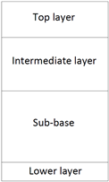 | 100 | Vegetable land | Vegetable land | Vegetable land |
| 150 | Limestone aggregates | Limestone aggregates | CDW | |
| 200 | Limestone aggregates | Expanded clay | Expanded clay | |
| 52 | Infiltration Cells | Infiltration Cells | Infiltration Cells |
| Sieve | 40 | 31.5 | 22.4 | 16 | 11.2 | 8 | 5.6 | 4 | 2 | 1 | 0.5 | 0.25 | 0.063 | |
|---|---|---|---|---|---|---|---|---|---|---|---|---|---|---|
| CDW | % pass | 100.0 | 95.0 | 62.0 | 60.0 | 50.0 | 40.0 | 36.0 | 30.0 | 20.0 | 16.0 | 15.0 | 10.0 | 5.0 |
| Vegetable land | %pass | 100.0 | 100.0 | 100.0 | 100.0 | 100.0 | 89.0 | 78.0 | 71.0 | 56.0 | 44.0 | 35.0 | 21.0 | 3.0 |
| Expanded clay | %pass | 100.0 | 100.0 | 100.0 | 100.0 | 95.0 | 59.0 | 25.0 | 1.9 | 1.0 | 0.0 | 0.0 | 0.0 | 0.0 |
| Limestone aggregates | %pass | 100.0 | 94.0 | 77.5 | 69.8 | 64.0 | 51.5 | 41.9 | 35.5 | 23.5 | 17.2 | 14.0 | 10.0 | 4.5 |
| Ambient Conditions | Wet Conditions | ||||||
|---|---|---|---|---|---|---|---|
| Material | (kg/m3) | λ (W/mK) | Ef (Ws1/2/m2K) | Cp (J/kgK) | λ (W/mK) | Ef (Ws1/2/m2K) | Cp (J/kgK) |
| Vegetable land | 1370 | 0.1422 | 449.89 | 1039 | 1.4121 | 1646.58 | 1280 |
| Limestone aggregate | 2400 | 1.8983 | 1721.66 | 651 | 2.3253 | 2081.07 | 745 |
| Recycled aggregate | 2100 | 1.4876 | 1473.48 | 695 | 2.0827 | 1901.03 | 723 |
| Expanded clay | 500 | 0.0982 | 309.58 | 1952 | 0.7101 | 921.95 | 1995 |
| Green Swale | Volume of Water Discharged (L) | Volume of Water Extracted (L) | Volume of Water Absorbed (L) |
|---|---|---|---|
| Type 1 | 122.7 | 99.3 | 23.4 |
| Type 2 | 152.6 | 113.6 | 39.0 |
| Type 3 | 146.1 | 108.5 | 37.6 |
| Green Swale | Dry Conditions | Wet Conditions | ||||||
|---|---|---|---|---|---|---|---|---|
| U (W/m2K) | Absolute Error (W/m2K) | Relative Error (%) | S (W/m2K) | U (W/m2K) | Absolute Error (W/m2K) | Relative Error (%) | S (W/m2K) | |
| Type 1 | 0.631 | 0.018 | 3.36 | 0.021 | 0.911 | 0.046 | 5.16 | 0.050 |
| Type 2 | 0.347 | 0.020 | 6.20 | 0.025 | 0.558 | 0.006 | 1.29 | 0.007 |
| Type 3 | 0.338 | 0.014 | 4.86 | 0.016 | 0.602 | 0.014 | 3.69 | 0.016 |
| Green Swale | Dry Conditions | Wet Conditions | ||||||
|---|---|---|---|---|---|---|---|---|
| λeq (W/mK) | Absolute Error (W/mK) | Relative Error (%) | S (W/mK) | λeq (W/mK) | Absolute Error (W/mK) | Relative Error (%) | S (W/mK) | |
| Type 1 | 0.284 | 0.009 | 3.36 | 0.010 | 0.410 | 0.023 | 5.16 | 0.025 |
| Type 2 | 0.156 | 0.010 | 6.20 | 0.012 | 0.251 | 0.003 | 1.29 | 0.004 |
| Type 3 | 0.152 | 0.007 | 4.86 | 0.008 | 0.271 | 0.007 | 3.69 | 0.008 |
| Thermal Conductivity (W/mK) | Dry Conditions | Wet Conditions |
|---|---|---|
| Vegetable land | 0.396 | 1.386 |
| Limestone aggregates | 0.268 | 0.816 |
| Expanded clay | 0.147 | 0.359 |
| CDW | 0.291 | 1.416 |
| Thermal Conductivity (W/mK) | Dry Conditions | Wet Conditions | ||
|---|---|---|---|---|
| Lower Bound | Upper Bound | Lower Bound | Upper Bound | |
| Vegetable land | 0.20 | 0.59 | 0.69 | 2.08 |
| Limestone aggregates | 0.13 | 0.40 | 0.41 | 1.22 |
| Expanded clay | 0.07 | 0.22 | 0.18 | 0.54 |
| CDW | 0.15 | 0.44 | 0.71 | 2.12 |
| Thermal Conductivity (W/mK) | Dry Conditions | Wet Conditions |
|---|---|---|
| Vegetable land | 0.373 | 0.963 |
| Limestone aggregates | 0.348 | 0.795 |
| Expanded clay | 0.105 | 0.298 |
| CDW | 0.315 | 0.711 |
| Green Swale | Dry Conditions | Wet Conditions |
|---|---|---|
| Type 1 | 2.270 | 2.776 |
| Type 2 | 1.772 | 2.522 |
| Type 3 | 1.765 | 2.544 |
Disclaimer/Publisher’s Note: The statements, opinions and data contained in all publications are solely those of the individual author(s) and contributor(s) and not of MDPI and/or the editor(s). MDPI and/or the editor(s) disclaim responsibility for any injury to people or property resulting from any ideas, methods, instructions or products referred to in the content. |
© 2023 by the authors. Licensee MDPI, Basel, Switzerland. This article is an open access article distributed under the terms and conditions of the Creative Commons Attribution (CC BY) license (https://creativecommons.org/licenses/by/4.0/).
Share and Cite
Rey-Mahía, C.; Álvarez-Rabanal, F.P.; Sañudo-Fontaneda, L.Á. Experimental and Numerical Study of the Thermal Properties of Dry Green Swales to Be Used as Part of Geothermal Energy Systems. Appl. Sci. 2023, 13, 10644. https://doi.org/10.3390/app131910644
Rey-Mahía C, Álvarez-Rabanal FP, Sañudo-Fontaneda LÁ. Experimental and Numerical Study of the Thermal Properties of Dry Green Swales to Be Used as Part of Geothermal Energy Systems. Applied Sciences. 2023; 13(19):10644. https://doi.org/10.3390/app131910644
Chicago/Turabian StyleRey-Mahía, Carlos, Felipe P. Álvarez-Rabanal, and Luis Á. Sañudo-Fontaneda. 2023. "Experimental and Numerical Study of the Thermal Properties of Dry Green Swales to Be Used as Part of Geothermal Energy Systems" Applied Sciences 13, no. 19: 10644. https://doi.org/10.3390/app131910644