Estimating Organic Matter Content in Hyperspectral Wetland Soil Using Marine-Predators-Algorithm-Based Random Forest and Multiple Differential Transformations

Abstract

To achieve a rapid and accurate estimation of the soil organic matter (SOM) content in wetland soil, we focused on surface soil samples from the Xianshan Lake wetland area in Zhejiang Province and proposed a novel method called Marine-Predators-Algorithm-Based Random Forest (MPARF) to establish a fast detection model for the SOM content. This study analyzed 85 soil samples from the study area with the aim of assessing the performance of various combinations of ten differential transformation methods and five regression algorithms in predicting the SOM content. Our research findings demonstrate that the combination of second-order differentiation (SD) and MPARF yields the best results, with the highest R² value (0.92) and the lowest RMSE (1.32 g/kg). Furthermore, we determined that the average SOM content in the study area’s soil is 9.77 g/kg. Additionally, we confirmed that different differential transformation methods contribute to improving the correlation between spectral data and the SOM content, thereby enhancing the development of predictive models. This study provides a robust methodology and foundation for future soil organic matter monitoring in the region.

1. Introduction

As a critical source of nutrients and a fundamental element of a soil’s energy, the soil organic matter (SOM) content describes the organic material that is present in soils. Changes in the SOM content, which is a key determinant of soil fertility, have a direct impact on the quantity of water and other microorganisms in the soil. These changes also have a significant effect on the biological, chemical, and physical characteristics of the soil [1]. Therefore, the rapid and accurate acquisition of the SOM content has become an inevitable need for modern agriculture development, which plays a vital role in maintaining ecological balance and promoting sustainable agricultural development. In the past few decades, methods for evaluating the SOM content have been thoroughly studied by researchers, and these methods may primarily be divided into two categories, i.e., conventional chemical technology and hyperspectral technology [2]. Due to their greater precision, stability, and dependability, traditional chemistry technologies are frequently used to determine the SOM content. But there are a lot of drawbacks, including cumbersome operation, environmental pollution, time-consuming and labor-intensive processes, and the need for experienced measurement personnel. Compared to conventional chemical technology, hyperspectral technology offers a number of benefits while retaining excellent accuracy, such as being easier to use, using fewer resources, performing analyses more quickly, and not polluting the environment. Specifically, hyperspectral techniques utilize soil spectral reflectance to capture the optical properties of soils at different wavelengths. By measuring and evaluating the spectral reflectance of soils, the physical and chemical qualities and properties of soils can be determined.

With the theory of hyperspectral technology gradually improving in recent years, it has been extensively used in the rapid estimation of the SOM content. In order to determine the SOM content of the Yinchuan Plain, Shang et al. [3] combined a variety of spectral transformation techniques with feature variable extraction techniques and established an estimation model of the SOM content using a variety of machine learning regression models to provide a theoretical foundation for the quick monitoring of the SOM content. In order to accurately and efficiently monitor the soil organic carbon content and the total soil nitrogen content in forest ecosystems, Wang et al. [4] collected 513 topsoil samples from northeastern China as research objects. They also made an effort to quickly predict the soil organic carbon and total soil nitrogen contents in dense vegetation cover areas using various machine learning models. The presence of environmental or human influence, which might introduce more or less noise into the data, is typically unavoidable during the collection of spectral data. Therefore, it is essential to preprocess the raw spectral reflectance data. At the moment, differential transform and wavelet transform are the major preprocessing techniques used for SOM spectral reflectance data. In their study, Huang et al. [5] focused on arid soil data and utilized a continuous wavelet transform with different scales to eliminate noise in the data. They combined it with a continuous projection algorithm for feature band extraction and used multiple regression methods to construct an inversion model of the soil organic carbon content. Wang et al. [6] conducted research employing soil samples from soils in Liaoning Province that were generated from loess parent material in order to quickly ascertain the organic matter content of the soil samples. To lessen the interference of noise in the experiment, they used a variety of spectral modification techniques on the original spectrum data and developed a hyperspectral prediction model to determine the organic matter content unique to the relevant area. Zhou et al. [7] conducted a study using 272 soil samples from the Three-River Source Region in the Qinghai–Tibetan Plateau. In order to properly estimate the soil organic carbon content, they attempted to build a hyperspectral inversion model to determine the best spectral transformation and model combination. The findings of their study provide a scientific basis for the rapid monitoring of the soil organic carbon content in high-altitude regions with cold climates. Similar related studies can be found in citations [8,9,10].

In summary, several researchers have combined various spectrum processing techniques with various machine learning prediction models to create inversion models using hyperspectral technology as a basis. These models are used to keep track of the SOM content in study areas. Although the above methods have achieved good performance in different regions and provided a corresponding scientific basis for the prediction of the SOM content in the study area, none of these methods were selected, or only individual differential transformation methods were selected for analysis and did not integrate and provide a detailed overview of the different differential transformation forms in order to compare which differential transformation methods can better model the inversion of the SOM. Additionally, all of the aforementioned techniques create hyperspectral inversion models for the respective areas using conventional machine learning regression techniques [11,12]. However, these models mostly necessitate setting model hyperparameters. The choice of hyperparameters has a crucial impact on the performance, convergence speed, and generalization ability of the model. By systematically trying different combinations of hyperparameters [13], the performance of the model can be optimized to better fit different datasets and tasks.

Therefore, this study collected differential methods that have emerged in recent years for predicting the soil organic matter content using hyperspectral data. These methods were combined with both unoptimized machine learning algorithms and an optimized Random Forest (RF) model for soil organic matter inversion. The aim was to explore the optimal model combination for predicting the soil organic matter content in the study area and to validate the effectiveness of this model. In this study, we first chemically processed and acquired hyperspectral data on soil samples from the wetlands of Zhejiang to derive the organic matter content of the soils in the region. Then, the spectral data were preprocessed via ten differential transforms and underwent SCARS screening for characteristic bands. The MPA-based RF algorithm was used to predict the soil organic matter content, and it was compared with the MLR, PLSR, SVR, and unoptimized RF models. The objectives of this study are as follows: (1) to analyze the effects of ten different differential transforms that are commonly used on spectral data and derive the best combination of algorithms for the region by combining different transforms with different models, and (2) to propose a soil organic matter detection method based on hyperspectral technology, which can be applied to laboratory hyperspectral data to realize the rapid detection of the soil organic matter content.

2. Materials and Methods

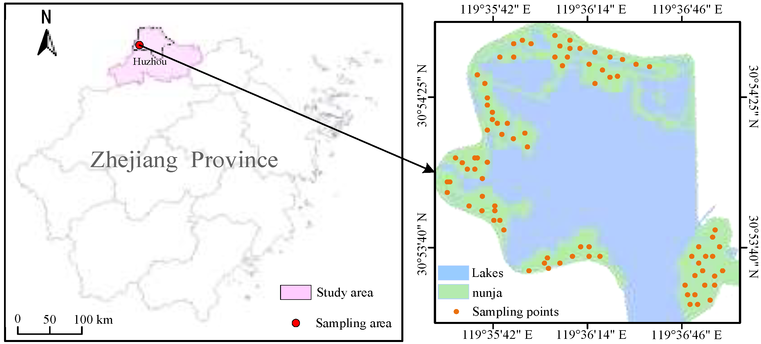
2.1. Collection and Testing of Soil Samples

The Xianshan Lake Wetland Park is located in Changxing County, Huzhou City, Zhejiang Province, China. It is situated in the northern part of Zhejiang Province and at the intersection of Zhejiang, Jiangsu, and Anhui provinces. The park covers an area of 2692.2 hectares. It is not only one of the largest wetlands in the province of Zhejiang’s north, but it is also one of the most ecologically diverse and unspoiled wetland ecosystems in the Yangtze River Delta, as well as a typical example of the natural wetlands and artificial lakes and wetland systems in Zhejiang. Its geographic structure is shown in Figure 1. The sample region has a diverse range of flora and animals, a thick canopy of vegetation, a subtropical monsoon climate, four distinct seasons, and a variety of landforms. It also has a moderate climate, plenty of sunshine, and abundant rainfall. The average annual temperature is 15.2 degrees Celsius, the average annual sunshine hours are 2074 h, and its soil types are mainly bog soil, paddy soil, and red earth soil.

The experimental soils in this study were collected in September 2022. A total of 85 soil sample points were collected from different types of 0–15 cm surface soils in the study area, of which five surface soil mixes were taken from each sample point. The well-blended soil samples were brought indoors for natural air drying. They were then ground to eliminate contaminants and underwent screening treatment using a sieve with a pore size of 2 mm. The soil samples were equally divided into two parts for soil spectral information collection and chemical technology for SOM content determination, in which the chemical technology utilized potassium dichromate oxidation to determine the SOM content [14]. The specific process of the chemical method was as follows: Under heating conditions, soil organic carbon was oxidized using an excess of potassium dichromate sulfuric acid solution. The excess potassium dichromate was titrated with a ferrous sulfate standard solution. The amount of potassium dichromate consumed was calculated according to the oxidation correction factor to determine the organic carbon content. This value was then multiplied by the constant 1.724 to obtain the SOM content.

Soil spectral reflectance was determined using an FX(17) hyperspectral camera with a spectral range of 900–1700 nm and a spectral resolution of 3.5 nm, containing a total of 224 bands. The spectral equipment acquisition device is shown in Figure 2. During the determination process, the light source was provided by six 50 W halogen lamps. The fiber optic probe had a field of view of 10°, and it was positioned at a distance of 20 cm from the surface of the soil samples. Each soil sample was divided into 27 portions and placed in a tray. Before the determination, each sample was calibrated with a white board to reduce instrument-related errors. Subsequently, based on ENVI5.3 software, 27 spectral curves were measured for each soil sample, and the average value was taken as the actual spectral curve for that soil sample after removing the outliers [15].

2.2. Spectral Data PreProcessing Methods for Soils

Soil spectral data preprocessing is a necessary data processing method that reduces the influence of factors such as noise, spurious signals, and non-linear spectral effects that are present in soil spectral data. It plays a crucial role in improving the accuracy and reliability of the data. This pretreatment approach can analyze soil samples without causing any damage. It provides more accurate, comprehensive, and efficient data information for soil analysis, which is crucial for supporting and ensuring the success of soil science research. In the field of soil science research, soil spectral data preprocessing has become a significant technological strategy that is widely employed in various areas including soil quality evaluation, analysis of soil organic matter content, and soil contamination detection. It plays a crucial role in improving the accuracy and reliability of soil analysis.

In this study, the raw soil spectral data were first subjected to SG smoothing. The SG smoothing [16] algorithm is a polynomial smoothing algorithm based on the principle of least squares proposed by Savitzky and Golay. It is an approach to signal processing that is frequently used to eliminate noise and spikes while keeping the data trend. The primary benefit of SG smoothing is its capacity to carry out smoothing and differentiation operations at the same time. SG smoothing has three parameters, namely window size, polynomial order, and derivative order. It can adapt to different data characteristics by adjusting the smoothing window size and polynomial order. When processing soil spectral data, SG smoothing efficiently eliminates random and systematic noise brought on by instrument measurement errors and environmental factors, enhancing the accuracy and quality of the resulting data. Additionally, it aids in lowering signal distortion and peak misalignment, improving the data’s capacity to be compared and understood. The theoretical formula for SG smoothing is as follows:

$${\tilde{\mathrm{x}}}_{\mathrm{i}}={\displaystyle \sum _{\mathrm{j}=-\mathrm{m}}^{\mathrm{m}}{\mathrm{c}}_{\mathrm{j}}{\mathrm{x}}_{\mathrm{i}+\mathrm{j}}},$$

(1)

where ${\tilde{\mathrm{x}}}_{\mathrm{i}}$ represents the value of the sample point after undergoing SG smoothing, ${\mathrm{x}}_{\mathrm{i}+\mathrm{j}}$ represents the value of the $\mathrm{i}+\mathrm{j}$ data point in the original data, $\mathrm{m}$ represents the order of the polynomial fit, and ${\mathrm{c}}_{\mathrm{j}}$ represents the coefficients of the fitted curve, which can be determined through the least squares method. By adjusting the polynomial order and coefficients, the smoothing degree and fitting accuracy of SG smoothing can be controlled. In this study, we set the derivative order to 0, the window size to 5, and the polynomial order to 3, which correspond to the five-point third-order smoothing method.

To further enhance the association between reflectance data and soil indicators, soil spectral data were further preprocessed utilizing a variety of differential transform techniques on the basis of SG smoothing. For this reason, this paper collects and organizes ten common methods of differential transformations in related papers in recent years, including first-order differentiation (FD), second-order differentiation (SD), logarithmic first-order differentiation (LFD), logarithmic second-order differentiation (LSD), inverse logarithmic first-order differentiation (RFD), inverse logarithmic second-order differentiation (RSD), log-logarithmic first-order differentiation (LRFD), log-logarithmic second-order differentiation (LRSD), inverse logarithmic first-order differentiation (RLFD), and inverse logarithmic second-order differentiation (RLSD). The spectra after LFD and LSD transformations can be theoretically shown to be equivalent to those after RLFD and RLSD transformations, and only the experimental results for RLFD and RLSD will be shown later in this section. The theoretical formulas for these differential transformation methods are shown in

Table 1. Differential transformation methods and their theoretical formulas.

Differential Transformation Method	Theoretical Formula	Differential Transformation Method	Theoretical Formula
FD	${\tilde{\mathrm{x}}}^{\prime }$	SD	${\tilde{\mathrm{x}}}^{″}$
LFD	$(\log \tilde{\mathrm{x}}{)}^{\prime }$	LSD	$(\log \tilde{\mathrm{x}}{)}^{″}$
RFD	$(1/\tilde{\mathrm{x}}{)}^{\prime }$	RSD	$(1/\tilde{\mathrm{x}}{)}^{″}$
LRFD	$(1/\log (\tilde{\mathrm{x}}){)}^{\prime }$	LRSD	$(1/\log (\tilde{\mathrm{x}}){)}^{″}$
RLFD	$(\log (1/\tilde{\mathrm{x}}){)}^{\prime }$	RLSD	$(\log (1/\tilde{\mathrm{x}}){)}^{″}$

, where $\log$ is the logarithm with base ‘e’, $\tilde{\mathrm{x}}$ represents the spectrums after SG smoothing, and ${•}^{\prime }$ and ${•}^{″}$ denote the first-order and second-order differentials, respectively.

2.3. Spectral Data Feature Band Selection

It is vital to perform feature band selection on the preprocessed soil hyperspectral data in order to draw out the most pertinent and important information from the vast array of spectral bands and lessen data redundancy and noise. In order to concentrate on certain spectral areas of interest and record the spectrum responses of target substances or characteristics, this selection process seeks to find the bands that are closely connected to the study objectives. This makes it easier to analyze the target components or traits quantitatively or qualitatively. The selection of feature bands not only lowers the cost of storing and processing data, but also increases the effectiveness and precision of model training. The link between spectral data and geophysical features is better understood since it makes it simpler for the model to learn and create correlations with the target. Common methods for feature band selection, as mentioned in [17], include successive projections algorithm (SPA), principal component analysis (PCA), Competitive Adaptive Reweighted Sampling (CARS), and SCARS. Among these methods, SCARS demonstrates significant advantages in dealing with high-dimensional data and complex problems. It effectively captures the intrinsic structure and relationships between features during the feature selection and sample resampling processes. It not only automatically adjusts the weights of samples based on their distribution, effectively handling imbalanced or noisy datasets, but also quickly converges to the global optimal solution. Moreover, it retains the maximum amount of information from the original data while keeping a smaller sample size, thereby improving the predictive performance and generalization ability of the model [18].

The computational process of using SCARS to find the optimal subset of variables in spectral data consists of N cyclic processes. In each iteration, SCARS first calculates the stability of each wavelength variable. Variables with larger stable values are then screened as a new subset of variables via Adaptive Reweighted Sampling and Exponentially Decreasing Function. After multiple iterations of selection, the final subset of variables is obtained. The Partial Least Squares Regression model is then applied to this final subset to calculate the root mean square error of cross-validation (RMSECV). Finally, the subset with the smallest RMSECV value is chosen as the optimal subset of variables, representing the optimal feature bands.

3. Models Overview

3.1. Traditional Machine Learning Model

3.1.1. Multiple Linear Regression (MLR)

MLR [19] is a statistical method that is widely used for data analysis and modeling. It predicts the value of a dependent variable by establishing a linear equation that includes multiple independent variables. MLR provides a linear relationship between the independent variables (spectral bands) and the dependent variable (SOM content). This makes the results of the model easier to interpret. It has been widely applied in the inversion of the soil organic matter content.

3.1.2. Partial Least Squares Regression (PLSR)

PLSR [20] is a multivariate regression analysis method based on principal component analysis. The fundamental idea of PLSR is to project the independent and dependent variables into separate new spaces in a way that maximizes the correlation between them in this new space. PLSR can effectively address the issue of multicollinearity in spectral data, simplify the complexity of the data, and can also improve the stability and modeling efficiency of the model. When modeling soil spectral data using PLSR, it is crucial to select an appropriate number of latent variables. Cross-validation is commonly used as an evaluation metric, and the visualization method is employed to determine the optimal number of latent variables. As a general rule, the cross-validation error tends to decrease initially and then increase as the number of latent variables increases. The optimal number of latent variables is usually the point at which the cross-validation error is minimized.

3.1.3. Support Vector Regression (SVR)

SVR [21] is a regression algorithm based on support vector machines. Due to the high dimensionality and noise interference in spectral data, traditional regression methods are prone to overfitting and underfitting issues. However, the SVR algorithm is capable of constructing a regression model in a high-dimensional space, which enhances its robustness and ability to capture complex relationships in the data. During the training process, the SVR algorithm aims to minimize the error between the predicted values and the true values. This makes it particularly effective in handling non-linear relationships between variables. The SVR model was constructed in MATLAB using the libSVM toolbox and the kernel function was set to the following radial basis kernel function:

$$\mathrm{k}({\mathrm{x}}_{\mathrm{i}},{\mathrm{x}}_{\mathrm{j}})=\exp \left(\frac{-\parallel {\mathrm{x}}_{\mathrm{i}}-{\mathrm{x}}_{\mathrm{j}}{\parallel }^2}{2{\mathsf{\delta }}^2}\right),$$

(2)

where $\mathrm{k}(•,•)$ represents the radial basis function, and $\mathsf{\delta }$ represents the width of the radial basis kernel. The penalty parameter and the width of the radial basis kernel in SVR are optimized through a grid search.

3.1.4. Random Forest (RF)

RF [22] is an ensemble learning algorithm based on decision trees. It consists of multiple decision trees, each trained using a different subsample and subset of features. RF is capable of fitting high-dimensional data well and has a certain degree of resistance to overfitting. In RF regression, the construction of each decision tree is random to ensure model diversity and generalization ability.

3.2. Marine-Predators-Algorithm-Based Random Forest

While the traditional machine learning models mentioned above have shown certain advantages in determining the SOM content, they often require significant computational resources to search for optimal parameters and often fail to find the best hyperparameters. Therefore, we propose Marine-Predators-Algorithm-Based Random Forest (MPARF) to enhance the performance and training speed of the RF model while reducing model overfitting. Specifically, due to the significant impact of the number of trees (ntree) and the maximum depth of trees (mdepth) on the accuracy of RF model, this study utilizes the MPA to optimize the parameters ntree and mdepth. The MPARF model is constructed to enhance the performance of RF in SOM content detection.

The MPA [23] is a novel metaheuristic optimization algorithm inspired by the behavior of marine predators. This algorithm mimics the predatory behavior and collective cooperation strategies observed in the ocean. The underlying concept of the MPA is to perform an optimization search by simulating the interactions between predators and prey in the ocean ecosystem. In the algorithm, the predators represent the candidate solutions in the search space, while the prey represents the optimal or local optimal solution of the problem. The optimization process of the MPA can be summarized as follows:

(1) Initialization stage: The MPA initiates the optimization process by initializing the positions of prey in the search space, as described by the following theoretical formula:

$${\mathrm{X}}_0={\mathrm{X}}_{\min }+\mathrm{rand}({\mathrm{X}}_{\max }-{\mathrm{X}}_{\min }),$$

(3)

where ${\mathrm{X}}_{\max },{\mathrm{X}}_{\min }$ is the search space range, and $\mathrm{rand}()$ is random number from 0 to 1.

(2) Optimization stage of MPA: The optimization stage consists of three scenarios that consider different velocity ratios and simulate the entire lifecycle of predators and prey.

The first scenario occurs when the velocity ratio is high or when the prey’s movement speed is higher than that of the predators. This situation occurs in the early iterations of the optimization process, when global search is crucial. In this stage, the optimal strategy for the predators is to maintain their current positions. The theoretical formula for the optimization process based on exploration strategy is as follows:

$$\begin{array}{c}{\mathrm{stepsize}}_{\mathrm{i}}={\mathrm{R}}_{\mathrm{B}}\otimes (\mathrm{E}\mathrm{l}\mathrm{i}\mathrm{t}{\mathrm{e}}_{\mathrm{i}}-{\mathrm{R}}_{\mathrm{B}}\otimes \mathrm{Pr}\mathrm{e}{\mathrm{y}}_{\mathrm{i}}),\\ \mathrm{Pr}\mathrm{e}{\mathrm{y}}_{\mathrm{i}}=\mathrm{Pr}\mathrm{e}{\mathrm{y}}_{\mathrm{i}}+\mathrm{P}\cdot \mathrm{R}\otimes \mathrm{s}\mathrm{t}\mathrm{e}\mathrm{p}\mathrm{s}\mathrm{i}\mathrm{z}{\mathrm{e}}_{\mathrm{i}},\\ \mathrm{I}\mathrm{t}\mathrm{e}\mathrm{r}<\frac{1}{3}\mathrm{MaxIter},\end{array}$$

(4)

where $\mathrm{i}=1,\dots \mathrm{n}$, $\mathrm{s}\mathrm{t}\mathrm{e}\mathrm{p}\mathrm{s}\mathrm{i}\mathrm{z}\mathrm{e}$ is the movement step size for this stage, ${\mathrm{R}}_{\mathrm{B}}$ is a Brownian walk random vector with normal distribution, and $\otimes$ represents the element-wise multiplication operator. This symbol simulates the movement of the prey. $\mathrm{P}$ is 0.5. $\mathrm{R}$ is a randomly and uniformly distributed value within the range [0, 1]. $\mathrm{E}\mathrm{l}\mathrm{i}\mathrm{t}{\mathrm{e}}_{\mathrm{i}}$ is an elite matrix composed of top-level predators. $\mathrm{I}\mathrm{t}\mathrm{e}\mathrm{r}$ is the current iteration number. $\mathrm{M}\mathrm{a}\mathrm{x}\mathrm{I}\mathrm{t}\mathrm{e}\mathrm{r}$ is the maximum number of iterations.

The second case is when the speed ratio is unified or when the predators and prey move at almost the same speed. This situation occurs during the middle phase of optimization iterations, where the population is divided into two parts. The prey in the algorithm performs Lévy flights to explore the search space, while the predators perform Brownian motion to explore, develop, and exploit the search space. The optimization process of the exploration and exploitation strategies can be described by the following theoretical formula:

$$\begin{array}{c}\mathrm{s}\mathrm{t}\mathrm{e}\mathrm{p}\mathrm{s}\mathrm{i}\mathrm{z}{\mathrm{e}}_{\mathrm{i}}={\mathrm{R}}_{\mathrm{L}}\otimes (\mathrm{E}\mathrm{l}\mathrm{i}\mathrm{t}{\mathrm{e}}_{\mathrm{i}}-{\mathrm{R}}_{\mathrm{L}}\otimes \mathrm{Pr}\mathrm{e}{\mathrm{y}}_{\mathrm{i}}),\\ \mathrm{Pr}\mathrm{e}{\mathrm{y}}_{\mathrm{i}}=\mathrm{Pr}\mathrm{e}{\mathrm{y}}_{\mathrm{i}}+\mathrm{P}\cdot \mathrm{CF}\otimes \mathrm{s}\mathrm{t}\mathrm{e}\mathrm{p}\mathrm{s}\mathrm{i}\mathrm{z}{\mathrm{e}}_{\mathrm{i}},\\ \frac{1}{3}\mathrm{M}\mathrm{a}\mathrm{x}\mathrm{I}\mathrm{t}\mathrm{e}\mathrm{r}<\mathrm{I}\mathrm{t}\mathrm{e}\mathrm{r}<\frac{2}{3}\mathrm{I}\mathrm{t}\mathrm{e}\mathrm{r},\end{array}$$

(5)

$$\begin{array}{c}\mathrm{s}\mathrm{t}\mathrm{e}\mathrm{p}\mathrm{s}\mathrm{i}\mathrm{z}{\mathrm{e}}_{\mathrm{i}}={\mathrm{R}}_{\mathrm{B}}\otimes ({\mathrm{R}}_{\mathrm{B}}\otimes \mathrm{E}\mathrm{l}\mathrm{i}\mathrm{t}{\mathrm{e}}_{\mathrm{i}}-\mathrm{Pr}\mathrm{e}{\mathrm{y}}_{\mathrm{i}}),\\ \mathrm{Pr}\mathrm{e}{\mathrm{y}}_{\mathrm{i}}=\mathrm{E}\mathrm{l}\mathrm{i}\mathrm{t}{\mathrm{e}}_{\mathrm{i}}+\mathrm{P}\cdot \mathrm{CF}\otimes \mathrm{s}\mathrm{t}\mathrm{e}\mathrm{p}\mathrm{s}\mathrm{i}\mathrm{z}{\mathrm{e}}_{\mathrm{i}},\\ \frac{1}{3}\mathrm{M}\mathrm{a}\mathrm{x}\mathrm{I}\mathrm{t}\mathrm{e}\mathrm{r}<\mathrm{I}\mathrm{t}\mathrm{e}\mathrm{r}<\frac{2}{3}\mathrm{I}\mathrm{t}\mathrm{e}\mathrm{r},\end{array}$$

(6)

where $\mathrm{i}=1,\dots \mathrm{n}/2,$ ${\mathrm{R}}_{\mathrm{L}}$ represents the Lévy flight random vector, and $\mathrm{CF}$ is the adaptive parameter for the movement step size of the predators, while the other parameters remain the same as mentioned above.

The third case is when the speed ratio is low, or when the predators move faster than the prey. This situation occurs in the later iterations of the optimization process. In this case, the optimal strategy for the predators is to perform a Lévy flight. The theoretical formula for this strategy is as follows:

$$\begin{array}{c}\mathrm{s}\mathrm{t}\mathrm{e}\mathrm{p}\mathrm{s}\mathrm{i}\mathrm{z}{\mathrm{e}}_{\mathrm{i}}={\mathrm{R}}_{\mathrm{L}}\otimes ({\mathrm{R}}_{\mathrm{L}}\otimes \mathrm{E}\mathrm{l}\mathrm{i}\mathrm{t}{\mathrm{e}}_{\mathrm{i}}-\mathrm{Pr}\mathrm{e}{\mathrm{y}}_{\mathrm{i}}),\\ \mathrm{Pr}\mathrm{e}{\mathrm{y}}_{\mathrm{i}}=\mathrm{E}\mathrm{l}\mathrm{i}\mathrm{t}{\mathrm{e}}_{\mathrm{i}}+\mathrm{P}\cdot \mathrm{CF}\otimes \mathrm{s}\mathrm{t}\mathrm{e}\mathrm{p}\mathrm{s}\mathrm{i}\mathrm{z}{\mathrm{e}}_{\mathrm{i}},\\ \mathrm{I}\mathrm{t}\mathrm{e}\mathrm{r}>\frac{2}{3}\mathrm{M}\mathrm{a}\mathrm{x}\mathrm{I}\mathrm{t}\mathrm{e}\mathrm{r},\end{array}$$

(7)

where the parameters have the same meanings as mentioned before.

(3) The vortex and fish aggregation device (FAD) strategy enables the MPA to overcome early convergence issues during the optimization process and avoid local optima. Its theoretical formula is as follows:

$$\mathrm{Pr}\mathrm{e}{\mathrm{y}}_{\mathrm{i}}\left\{\begin{array}{l}\mathrm{Pr}\mathrm{e}{\mathrm{y}}_{\mathrm{i}}+\mathrm{C}\mathrm{F}[{\mathrm{X}}_{\min }+{\mathrm{R}}_{\mathrm{L}}\otimes ({\mathrm{X}}_{\max }-{\mathrm{X}}_{\mathrm{minn}})]\otimes \mathrm{U}\mathrm{r}\\ \mathrm{Pr}\mathrm{e}{\mathrm{y}}_{\mathrm{i}}+[\mathrm{FADs}(1-\mathrm{r})+\mathrm{r}](\mathrm{Pr}\mathrm{e}{\mathrm{y}}_{\mathrm{r}1}-\mathrm{Pr}\mathrm{e}{\mathrm{y}}_{\mathrm{r}2})\mathrm{r}\end{array}\right.\begin{array}{l}\mathrm{r}\le \mathrm{FADs}\\ \mathrm{r}>\mathrm{FADs}\end{array}$$

(8)

where $\mathrm{FADs}$ is equal to 0.2, and $\mathrm{U}$ is a binary array.

The specific steps of the MPARF algorithm are as follows: The population size of the MPA is set to 20, and the maximum number of iterations is set to 200. The values of the other parameters, such as FDAs, are also set. The algorithm’s execution is controlled by comparing the current iteration count with the maximum iteration count. The model calculation steps are shown in Figure 3.

3.3. Model Evaluation

The predictive model’s accuracy was evaluated using the coefficient of determination (R²), root mean square error (RMSE), and relative percent deviation (RPD). The R² value represents the goodness of fit of the model and ranges from 0 to 1. A value closer to 1 indicates a more accurate simulation of the corresponding model. The RMSE represents the dispersion of the model, with a smaller RMSE indicating a better fit and a larger RMSE indicating a poorer fit. The RPD represents the reliability of the model. When the RPD is less than 1.5, the model is considered unreliable; when the RPD is between 1.5 and 2.0, the model is considered relatively reliable; and when the RPD is greater than 2.0, the model is considered highly reliable and suitable for model interpretation [24]. In summary, a good predictive model will have an R² value closer to 1, a smaller RMSE, and a larger RPD. The theoretical formula is as follows:

$${\mathrm{R}}^2=1-\frac{{\displaystyle {\sum }_{\mathrm{i}=1}^{\mathrm{n}}{({\mathrm{y}}_{\mathrm{i}}-{\tilde{\mathrm{y}}}_{\mathrm{i}})}^2}}{{\displaystyle {\sum }_{\mathrm{i}=1}^{\mathrm{n}}{({\mathrm{y}}_{\mathrm{i}}-\overline{\mathrm{y}})}^2}},$$

(9)

$$\mathrm{RMSE}=\sqrt{\frac{1}{\mathrm{n}}{\displaystyle \sum _{\mathrm{i}=1}^{\mathrm{n}}{({\mathrm{y}}_{\mathrm{i}}-{\tilde{\mathrm{y}}}_{\mathrm{i}})}^2}},$$

(10)

$$\mathrm{R}\mathrm{P}\mathrm{D}=\frac{\mathrm{SD}}{\mathrm{RMSE}},$$

(11)

where ${\mathrm{y}}_{\mathrm{i}}$ is the measured value, ${\tilde{\mathrm{y}}}_{\mathrm{i}}$ is the model prediction, $\overline{\mathrm{y}}$ is the mean value of the sample, $\mathrm{n}$ is the number of samples, and $\mathrm{SD}$ is the standard deviation of the analyzed samples.

3.4. Research Route

The research process was divided into four main parts: data collection, data preprocessing, spectral data analysis, and model building and evaluation. The research process is summarized in Figure 4. Firstly, soil samples were collected from the research area for determination of the SOM content via chemical methods, and the spectral data are determined via a hyperspectral camera. Secondly, the acquired spectral data were processed using ENVI5.3 software to standardize and correct them, eliminating excessive high and low bands that were present in the data. The data were then preprocessed using SG smoothing for denoising and spectral differential transforms. Subsequently, the preprocessed data were analyzed to determine the SOM content, spectral curve characteristics, and correlation between variables. The SCARS algorithm was then employed to select the feature bands from the data. Finally, five different algorithms were utilized to establish SOM inversion models, and these models were evaluated using metrics such as R² to assess their performance. In the research, the implementation of differential transformations, SCARS, and the five models were all based on the MATLAB 2020 platform. The experimental environment was as follows: Intel(R) Core^TM i5-9400 CPU @ 2.90GH8 GB RAM, 64 bit Windows 10, and MatlabR2020a. The SCARS algorithm was implemented using the carspls Toolbox, while the SVR algorithm was implemented using the libSVM Toolbox. The MLR, PLSR, RF, and MPARF algorithms all make use of the Statistics and Machine Learning Toolbox.

4. Results

4.1. Statistical Analysis of Soil Organic Matter Content

In this article, the 85 soil samples were randomly divided, with 70% of the samples (59 samples) used as the training set and 30% of the samples (26 samples) used as the testing set. The outcomes of the statistical analysis performed on the soil samples are shown in

Table 2. Statistics of SOM content/(g/kg).

Statistics	Number of Samples	Maximum Value	Minimum Value	Mean Value	Standard Deviation	Coefficient of Variation
Total sample	85	19.40	3.68	9.77	3.80	38.94
Training sample	59	18.50	5.03	9.68	3.53	36.56
Testing sample	26	19.40	3.68	9.81	3.97	40.54

. The SOM content in the study area ranges from a minimum of 3.68 g/kg to a maximum of 19.40 g/kg, with an average value of 9.77 g/kg. The standard deviation is 3.80 g/kg, and the coefficient of variation is 38.94%, indicating a moderate level of variability. The means of the soil organic matter content in the training and testing samples are 9.68 g/kg and 9.71 g/kg, respectively, with standard deviations of 3.53 g/kg and 3.97 g/kg. The coefficient of variation values for the training and testing samples are 36.56% and 40.54%, respectively, indicating a moderate level of variability. The mean and standard deviation of the organic matter content in the training and testing samples are overall similar, suggesting the feasibility of modeling. Figure 5 illustrates that the SOM content in the study area follows a normal distribution and falls between the ranges of the training and testing samples. This indicates that random partitioning can be used to establish training and testing samples for modeling and provides a solid data foundation for the models developed in this study.

4.2. Soil Spectral Profile Characterization

The visualization results of the original soil spectral data compared to the original spectral curve are shown in Figure 6. From the spectral curves of the soil samples, it can be observed that within the wavelength range of 900 to 1700 nm, the reflectance curves exhibit a similar overall trend for all of the soil samples. The spectral reflectance values of the soil samples range between 0.15 and 0.6. As shown in Figure 6, the spectral reflectance continuously increases in the range of 900–1400 nm. This may be due to the interaction between the chemical bonds in the molecular structure of soil components and near-infrared light. The wavelength range of 900–1400 nm has a strong penetration capability. The organic matter molecules in the soil exhibit strong absorption of near-infrared light. The spectral reflectance remains relatively stable in the range of 1420–1680 nm. This is mainly because the spectral characteristics within this range have weak interactions with the functional groups and chemical bonds in the molecular structure of soil organic matter. Additionally, the spectral characteristics in this range are influenced by water and other soil components, leading to higher stability in the spectral reflectance of the SOM. Moreover, there is a prominent absorption peak at 1420 nm, which is primarily influenced by the O-H molecules in the soil. The vibration of the C-H bonds in the organic matter molecules generates a typical 1.4 µm absorption band, which can be detected using spectroscopic instruments and manifested as a distinct absorption peak.

4.3. Correlation Analysis of Organic Matter Content with Different Spectral Transformation Forms

As described in Section 2.2, the soil spectral data in this study underwent several preprocessing steps. Firstly, the original spectral curves were subjected to SG smoothing. Then, several spectral transformations, including FD, SD, RFD, RSD, LRSD, LRSD, RLFD, and RLSD, were used. Figure 7 displays the visible outcomes of these modifications.

To further investigate the correlation between the transformed spectral reflectance and the measured SOM content, an analysis was conducted on the results of SG smoothing and the eight transformations for the first sample. The visual results are presented in Figure 8. In Figure 8, it can be observed that the original spectral curve, N, exhibited a negative correlation with the organic matter content, and the correlation coefficient curve was relatively smooth. By combining Figure 8 and

Table 3. Correlation coefficient values between SOM content and different spectral transformation forms.

Spectral Transformation Form	N	FD	SD	RFD	RSD	LRFD	LRSD	RLFD	RLSD
Maximum value	0.01	0.55	0.35	0.38	0.37	0.24	0.33	0.43	0.40
Minimum value	−0.10	−0.38	−0.33	−0.54	0.42	−0.51	−0.30	−0.53	−0.39

, it is evident that the FD transformation yielded the highest correlation coefficient value, with an absolute value of 0.55. Additionally, all of the differential transformation curves exhibited significant fluctuations around 1400 nm, indicating the presence of minor absorption valleys influencing the spectral absorption in that region. The correlation coefficients between the SOM and the original spectra after being transformed by RFD, LRFD, and RLFD exhibited a negative correlation. The absolute values of their maximums are 0.52, 0.51, and 0.53, respectively, with significant fluctuations in the curve transformations. On the other hand, the shapes of the curves are relatively similar after the transformations via SD, LRSD, and RLSD. The correlation coefficients for these transformations are all in the range of −0.4 to 0.4, indicating a weak correlation between the transformed values and SOM. On the other hand, the RSD transformation showed positive correlation coefficients, indicating a positive relationship with the SOM. The curve fluctuations for RSD transformation are relatively small. The different forms of differential transformation significantly improved the correlation between the soil spectral reflectance and the SOM content. This shows that the spectral data processed using the differential transformation method can be effectively used for modeling the SOM content.

4.4. Extraction of Feature Bands Using SCARS Algorithm

In this study, the SCARS algorithm was applied to extract the feature bands from the spectral data after eight spectral transformations. Specifically, the feature bands of the original spectrum N, after SG smoothing and denoising, were selected for further analysis. As shown in Figure 9a, the number of variables selected by SCARS decreases exponentially with the number of runs in 250 samples. The overall trend exhibited a rapid decrease, followed by a gradual stabilization. As shown in Figure 9b,c, the root mean square error of RMSECV exhibits a gradual decrease overall, indicating that the eliminated bands during the screening process are not significantly related to the SOM content. The RMSECV reaches its minimum value of 2.599 in the 173rd iteration, with a total of nine variables screened. After this point, the RMSECV starts to increase.

In order to provide a detailed comparison of the characteristic bands selected using different spectral transformation methods using the SCARS algorithm,

Table 4. Selected feature bands for various spectral transformations after running the SCARS.

Spectral Transformation Form	Feature Band/nm
N	946, 1034, 1038, 1045, 1055, 1199, 1214, 1344, 1375, 1428
FD	1077, 1081, 1095, 1116, 1275, 1278, 1402, 1469, 1522, 1604, 1611, 1681
SD	996, 1003, 1188, 1213, 1227, 1234, 1241, 1255, 1273, 1280, 1333, 1337, 1351, 1401, 1426, 1433, 1436, 1440, 1465, 1472, 1507, 1525, 1539, 1557, 1568, 1575, 1582, 1603, 1653, 1656, 1681, 1685
RFD	1176, 1183, 1257, 1264, 1459, 1522, 1568
RSD	971, 996, 1010, 1213, 1227, 1241, 1255, 1294, 1383, 1397, 1426, 1433, 1436, 1440, 1504, 1507, 1525, 1582, 1653
LRFD	1095, 1116, 1119, 1179, 1183, 1275, 1278, 1324, 1399, 1423, 1430, 1459, 1469, 1522, 1529, 1604, 1607, 1681
LRSD	996, 1003, 1188, 1220, 1255, 1273, 1305, 1337, 1372, 1397, 1426, 1433, 1436, 1440, 1472, 1507, 1525, 1568, 1582, 1653, 1656, 1681
RLFD	971, 1073, 1112, 1176, 1183, 1194, 1257, 1264, 1275, 1278, 1459, 1469, 1505, 1522, 1568, 1611
RLSD	996, 1213, 1241, 1255, 1266, 1397, 1426, 1433, 1436, 1440, 1472, 1525, 1568, 1582, 1653, 1681

presents a comprehensive list of the selected characteristic bands for each spectral transformation. According to Table 4, after applying the SCARS algorithm, the N, FD, SD, RFD, RSD, LRFD, LRSD, RLFD, and RLSD transformations yielded 10, 12, 32, 7, 19, 18, 22, 16, and 16 characteristic bands, respectively. The selection of characteristic bands compressed the input bands to less than 14.29% of the total number of bands.

It effectively extracted significantly different spectral features and reduced the data dimensionality, thereby improving the speed of model execution. Overall, the characteristic bands selected by the eight spectral transformations mainly concentrated in the near-infrared spectral range of 1100–1500 nm. This may be attributed to the absorption valleys caused by the chemical components in the soil in the near-infrared region. Among them, the SD transformation resulted in the highest number of selected characteristic bands, capturing relevant information in each wavelength range. On the other hand, the RFD transformation yielded the fewest characteristic bands, and it can be observed from the table that some bands were included in the characteristic bands selected by the RLFD transformation. This is because the reciprocal logarithmic first-order differentiation transformation emphasizes bands with larger logarithmic derivative values and is mainly used to extract broader spectral features. Conversely, the reciprocal logarithmic first-order differentiation transformation can better highlight local features in the spectrum, resulting in more detailed and accurate characteristic bands. The characteristic bands selected by the LRFD and LRSD transformations were mainly concentrated in the range of 1400–1600 nm, reflecting the detailed information and local changes in the spectrum. In this wavelength range, the absorption peak of the soil organic matter can be highlighted and accentuated by the logarithmic reciprocal differentiation transformation.

4.5. Comparative Analysis of Soil Organic Matter Content Inversion Model Accuracy

The sensitive bands selected by the SCARS algorithm were used as input variables for the inversion models, with the SOM content as the dependent variable. The MLR, PLSR, SVR, RF, and MPARF methods were used to construct the soil organic matter content prediction models. The experimental results are shown in

Table 5. Comparison of accuracy of SOM content inversion models.

Spectral Transformation Form	Model	Training Set			Testing Set
		R2	RMSE	RPD	R2	RMSE	RPD
N	MLR	0.62	2.16	1.63	0.51	3.12	1.43
	PLSR	0.60	2.27	1.59	0.60	2.62	1.58
	SVR	0.53	2.71	1.45	0.44	2.57	1.34
	RF	0.36	2.95	1.25	0.27	3.29	1.17
	MPARF	0.70	2.02	1.82	0.65	2.58	1.77
FD	MLR	0.76	1.91	2.05	0.66	2.56	1.72
	PLSR	0.73	1.82	1.94	0.69	2.18	1.79
	SVR	0.77	1.65	2.08	0.63	2.72	1.64
	RF	0.85	1.51	2.61	0.59	2.26	1.56
	MPARF	0.88	1.47	2.80	0.86	1.55	2.40
SD	MLR	0.85	1.40	2.59	0.61	2.52	1.60
	PLSR	0.70	2.08	2.98	0.65	2.32	1.70
	SVR	0.54	2.87	1.48	0.49	2.96	1.39
	RF	0.52	2.71	1.44	0.39	2.98	1.28
	MPARF	0.92	1.27	3.14	0.90	1.32	3.02
RFD	MLR	0.70	2.02	1.83	0.63	2.49	1.65
	PLSR	0.75	2.00	1.98	0.67	2.20	1.73
	SVR	0.69	2.21	1.80	0.58	2.24	1.54
	RF	0.80	1.66	2.23	0.70	2.00	1.82
	MPARF	0.85	1.41	2.57	0.78	1.80	2.11
RSD	MLR	0.63	2.19	1.65	0.54	2.54	1.47
	PLSR	0.77	1.84	2.09	0.75	1.83	2.00
	SVR	0.68	2.28	1.77	0.75	1.54	2.02
	RF	0.61	2.34	1.60	0.57	2.50	1.52
	MPARF	0.90	1.32	1.27	0.85	1.42	2.40
LRFD	MLR	0.82	1.52	2.35	0.72	2.26	1.89
	PLSR	0.74	1.99	1.98	0.74	1.79	1.94
	SVR	0.76	1.91	2.05	0.63	2.16	1.65
	RF	0.71	1.75	1.86	0.53	2.97	1.47
	MPARF	0.84	1.46	2.57	0.77	1.75	2.03
LRSD	MLR	0.74	1.97	1.94	0.64	2.09	1.67
	PLSR	0.77	1.74	2.08	0.73	1.98	1.94
	SVR	0.66	2.20	1.71	0.58	2.50	1.54
	RF	0.61	2.13	1.60	0.55	2.96	1.48
	MPARF	0.88	1.36	2.97	0.85	1.53	2.55
RLFD	MLR	0.77	1.89	2.09	0.68	2.05	1.76
	PLSR	0.83	1.56	2.39	0.52	2.71	1.44
	SVR	0.81	1.59	2.32	0.66	2.41	1.71
	RF	0.74	1.84	1.95	0.75	2.10	2.00
	MPARF	0.89	1.41	2.88	0.81	1.54	2.31
RLSD	MLR	0.71	2.06	1.87	0.67	2.07	1.74
	PLSR	0.81	1.58	2.31	0.76	1.87	2.04
	SVR	0.75	1.69	2.01	0.69	2.48	1.78
	RF	0.63	2.13	1.63	0.52	3.01	1.44
	MPARF	0.91	1.31	3.11	0.87	1.35	2.94

. From Table 5, it can be observed that there are differences in the prediction results among different spectral transformation methods. However, considering the overall evaluation criteria, both for the training set and the testing set, the experimental results of the spectral data after undergoing the eight spectral transformations are superior to those of the original spectra without any transformation. Furthermore, among the five prediction models, MPARF demonstrates better experimental results and stability compared to the other four models, indicating its ability to predict the soil organic matter content in the study area more effectively.

Among all the combinations of spectral transformations and inversion models, the SD-MPARF and RLSD-MPARF models performed well on both the training and testing sets, while the N-RF and N-SVR models yielded poorer results. This could be due to the presence of noise in the original spectra or the limited extraction of informative spectral bands. Overall, the MPARF model demonstrated high stability and fitting performance on both the training and testing sets. The MLR and PLSR models showed high stability but had inferior predictive results compared to MPARF. The SVR model and the unoptimized RF model exhibited highly unstable performance. The overall estimation performance of the five models, ranked from high to low, was MPARF > PLSR > MLR > SVR > RF. This could be attributed to the high linear relationship between the soil types and organic matter content in the study area, resulting in the linear models performing better than the non-linear models. The poor performance of the RF model may be attributed to a low number of features or low correlation between the features and variables. Due to its adaptability, the MPA can adjust its search strategy based on the problem’s characteristics and data features, allowing for it to be flexibly applied to different regression prediction problems and find the optimal configuration for the RF model. Considering each individual model, various spectral transformation combinations showed good fitting performances. The MLR model based on LRSD spectral transformation exhibited good prediction results, with a training set R² value of 0.82, a testing set R² value of 0.72, and a mean RPD of 2.11. The PLSR model based on SD spectral transformation showed good prediction performance, with a training set R² value of 0.88, a testing set R² value of 0.65, and a mean RPD of 2.40. The SVR model based on RLSD spectral transformation demonstrated good prediction performance, with a training set R² value of 0.81, a testing set R² value of 0.66, and a mean RPD of 2.02. The RF model based on RSD spectral transformation yielded good prediction results, with a training set R² value of 0.80, a testing set R² value of 0.70, and a mean RPD of 2.03. The MPARF models based on various differential transformations all outperformed the prediction of untreated spectral data, exhibiting higher stability and accuracy than the other models, with training and testing set R² values exceeding 0.85.

Based on the results of the eight spectral transformations, the MPARF, RSD-SVR, RSD-PLSR, RLFD-RF, RLFD-PLSR, and MPA-RF models exhibited testing set RPD values above 2.0, indicating strong reliability and more trustworthy prediction results. On the other hand, the N-SVR, N-RF, SD-SVR, and SD-RF models had testing set RPD values below 1.4, suggesting lower reliability of the models established using these methods. The remaining models had RPD values ranging from 1.4 to 2.0, indicating a moderate level of reliability and the ability to provide rough estimations of the SOM content in the study area.

Based on the above, different spectral transformation methods can improve the modeling accuracy to varying degrees. Spectral transformation alters the characteristics of the original spectral data, thereby influencing the performance of the models. Therefore, taking the MPARF model with better experimental results as an example, this study presents the model fitting accuracy plots for various spectral transformations, as shown in Figure 10. Overall, the predicted values for the training and testing sets are mostly distributed around the 1:1 line, indicating good prediction results. Among the individual spectral transformations, the SD transformation exhibits the best fit for the training set, with an R² value of 0.92. This may be attributed to the ability of the SD transformation to enhance the peak and valley information in the spectral data, thereby improving the discrimination of different components and helping the MPARF model to establish a better relationship between the SOM content and spectral data.

5. Discussion

Numerous studies have demonstrated that spectral transformations can reduce noise in the original spectral data, improve the discriminability of spectral data, and enhance data interpretability [25,26]. In order to improve the predictive accuracy of the model, this study applied various forms of differential transformations to the original spectral data of the study area. The results show that differential transformations can enhance the correlation between spectral reflectance and the SOM content. The correlation between the original data and the SOM was less than 0.1, but after preprocessing, the correlation was increased to a maximum of 0.54. Individual differential transformation methods can highlight features such as slopes, peaks, and valleys in the spectrum, thereby increasing the correlation between the organic matter content and reflectance. Second-order differential transformation, compared to first-order differential transformation, can provide a better estimation of the soil organic matter content in the study area, which is consistent with the findings of Zhou et al. [27]. The combination of reciprocal logarithm and differential transformation can enhance the features of the spectral signal and reduce the influence of background interference and noise on the spectral data, which is in line with the results obtained by Shen et al. [28].

This study found that the correlation coefficient between the soil spectra and the organic matter content in the study area is less than 0.1. Therefore, it is challenging to select feature bands based on the original spectral data. Previous researchers have used methods such as correlation coefficient analysis [29] or variance analysis [30] to study the relationship between the soil properties and soil spectral reflectance, selecting bands with high correlation coefficients or high variance contributions as feature bands. Currently, many scholars use methods like successive projections algorithm, principal component analysis, or CARS for feature band selection. In this study, the SCARS algorithm was employed to extract feature bands. The research shows that the SCARS algorithm can remove redundant information from the original spectral data and reduce the number of bands. For different spectral transformation methods, the SCARS algorithm selected feature bands that accounted for less than 14.29% of the full spectrum, thereby addressing the issue of input variables in the model. In previous studies on the spectral inversion of the soil organic matter content, differential transformation has been a commonly used spectral preprocessing method, and SCARS has also been widely used for feature wavelength selection. PLSR, SVR, and RF are widely used inversion model algorithms. From the above five models, both linear models, MLR and PLSR, exhibit greater stability compared to the non-linear models, SVR and RF. This may be attributed to the relatively uniform distribution of the soil organic matter content in the study area and the presence of linear relationships. Among these models, the RF model shows the least stable prediction accuracy, with an accuracy of only 0.36 using the original spectra. After applying RFD transformation, the prediction accuracy increases to 0.80. This instability in the RF model could be due to its inherent randomness. However, by using optimization algorithms to adjust the hyperparameters of the RF model, its stability can be improved [31]. In contrast to RF, MPARF not only enhances the original RF model’s performance but also exhibits improved stability. It is worth noting that our dataset was relatively small, and MPARF was validated on limited laboratory hyperspectral data, limiting its generalizability. Additionally, further investigations could apply this method to aerial hyperspectral data in the study area to demonstrate its broader applicability.

6. Conclusions

This article focused on predicting the soil organic matter content using soil samples from the Xianshan Lake wetland in Zhejiang Province. The actual organic matter content of the samples was measured using chemical methods, and the spectral data of the samples was obtained using a laboratory spectrometer. After preprocessing the spectral data using eight spectral differentiation transformation methods, the SCARS algorithm was applied to select the characteristic bands for feature extraction. Five inversion models, including MLR, PLSR, SVR, RF, and MPARF, were constructed. By comparing the simulation accuracy and stability of these models, this study aimed to determine the optimal combination of spectral transformation methods and models for predicting the soil organic matter content. The main conclusions are as follows:

(1) The optimization of the Random Forest (RF) model using the Marine Predators Algorithm (MPA) effectively improves the performance of the RF model, enhancing the accuracy and generalization ability of regression predictions. The MPA allows for global search in the solution space, maintaining diversity and exploration capabilities. It possesses adaptability and flexibility, enabling it to find optimal parameter configurations for the RF model and improve regression predictions. The predictive accuracy of the model is significantly enhanced, demonstrating high stability and accuracy. SD-MPARF exhibits accuracy comparable to the chemical methods, with the highest R² value (0.92) and the lowest RMSE (1.27 g/kg).

(2) The soil organic matter content in the study area ranges from 3.68 to 19.40 g/kg, with an average of 9.77 g/kg, indicating a relatively low organic matter content. As a result, the correlation coefficient between the high-spectral data and organic matter content is relatively low.

(3) The correlation coefficients between the original spectral reflectance and the soil organic matter content significantly increase after various spectral differentiation transformations. The correlation coefficient improves from 0.1 for the original spectral data to 0.55, indicating that different forms of differentiation transformations highlight detailed information and local variations in the spectra while weakening the noise and background signals, thereby enhancing the discriminability of the spectral features.

(4) The feature bands selected by the SCARS algorithm account for less than 14.29% of the full spectrum. This algorithm dynamically adjusts feature weights and selects feature bands with significant discriminatory power, greatly reducing redundant information in the spectral data and improving the modeling speed.

Of course, this paper also has some limitations. For example, Xianshan Lake may not represent wetland parks in the entire Zhejiang region. In the future, we plan to collect data from more diverse wetland parks in different regions to conduct a more comprehensive study. Additionally, the machine learning algorithms used in this paper, while classic, are relatively older. In the future, we intend to combine more advanced and comprehensive regression models to build more robust inversion models.

References

1. Murphy, B. Key soil functional properties affected by soil organic matter-evidence from published literature. In Proceedings of the IOP Conference Series: Earth and Environmental Science, Bendigo, VIC, Australia, 24–27 March 2014. [Google Scholar]
2. Angelopoulou, T.; Balafoutis, A.; Zalidis, G.; Bochtis, D. From Laboratory to Proximal Sensing Spectroscopy for Soil Organic Carbon Estimation—A Review. Sustainability 2020, 12, 443. [Google Scholar] [CrossRef]
3. Shang, T.; Mao, H.; Zhang, J.; Cheng, R.; Wang, F.; Jia, K. Hyperspectral estimation of soil organic matter content in Yinchuan plain, China based on PCA sensitive band screening and SVM modeling. Chin. J. Ecol. 2021, 40, 4128–4136, (In Chinese with English Abstract). [Google Scholar]
4. Wang, S.; Zhuang, Q.; Jin, X.; Yang, Z.; Liu, H. Predicting Soil Organic Carbon and Soil Nitrogen Stocks in Topsoil of Forest Ecosystems in Northeastern China Using Remote Sensing Data. Remote Sens. 2020, 12, 1115. [Google Scholar] [CrossRef]
5. Huang, X.; Wang, X.; Baishan, K.; An, B. Hyperspectral Estimation of Soil Organic Carbon Content Based on Continuous Wavelet Transform and Successive Projection Algorithm in Arid Area of Xinjiang, China. Sustainability 2023, 15, 2587. [Google Scholar] [CrossRef]
6. Wang, J.; Yang, W.; Wang, Y.; Xu, X.; Han, C.; Wang, Q. A Hyperspectral prediction model for organic matter content in soil developed from Loess-like parent material in Liaoning Province. Chin. J. Soil. Sci. 2022, 53, 1320–1330, (In Chinese with English Abstract). [Google Scholar]
7. Zhou, W.; Li, H.; Wen, S.; Xie, L.; Wang, T.; Tian, Y.; Yu, W. Simulation of Soil Organic Carbon Content Based on Laboratory Spectrum in the Three-Rivers Source Region of China. Remote Sens. 2022, 14, 1521. [Google Scholar] [CrossRef]
8. Zhang, Z.; Ding, J.; Wang, J. Spectral Characteristics of Oasis Soil in Arid Area Based on Harmonic Analysis Algorithm. Acta Opt. Sin. 2019, 39, 0228003. [Google Scholar] [CrossRef]
9. Chen, C.; Dai, H.; Feng, Y.; Yang, Z.; Yang, J. Setinel-2A based inversion of the organic matter content of soil the Sunwu area. Geophys. Geochem. Explor. 2022, 46, 1141–1148. [Google Scholar]
10. Liu, T.; Zhu, X.; Bai, X.; Peng, Y.; Li, M.; Tian, Z.; Jiang, Y.; Yang, G. Hyperspectral estimation model construction and accuracy comparison of soil organic matter content. Smart Agric. 2020, 2, 129–138. [Google Scholar]
11. Choudhury, B.U.; Divyanth, L.G.; Chakraborty, S. Land use/land cover classification using hyperspectral soil reflectance features in the Eastern Himalayas. India. Catena. 2023, 229, 107200. [Google Scholar] [CrossRef]
12. Chang, N.; Jing, X.; Zeng, W.; Zhang, Y.; Li, Z. Soil Organic Carbon Prediction Based on Different Combinations of Hyperspectral Feature Selection and Regression Algorithms. Agronomy 2023, 13, 1806. [Google Scholar] [CrossRef]
13. Claesen, M.; De Moor, B. Hyperparameter search in machine learning. arXiv 2015, arXiv:1502.02127. [Google Scholar]
14. Walkley, A.; Black, I.A. An examination of the Degtjareff method for determining soil organic matter, and a proposed modification of the chromic acid titration method. Soil Sci. 1934, 37, 29–38. [Google Scholar] [CrossRef]
15. Zhang, M.; Wang, S.; Li, S.; Yi, J.; Fu, P. Prediction and map-making of soil organic matter of soil profile based on imaging spectroscopy: A case in Hubei China. In Proceedings of the 2011 19th International Conference on Geoinformatics, Shanghai, China, 24–26 June 2011; pp. 1–5. [Google Scholar]
16. Zhao, A.; Tang, X.; Zhang, Z.; Liu, J. The parameters optimization selection of Savitzky-Golay filter and its application in smoothing pretreatment for FTIR spectra. In Proceedings of the 2014 9th IEEE Conference on Industrial Electronics and Applications, Hangzhou, China, 9–11 June 2014; pp. 516–521. [Google Scholar]
17. Yun, Y.H.; Li, H.D.; Deng, B.C.; Cao, D.S. An overview of variable selection methods in multivariate analysis of near-infrared spectra. Trends Anal. Chem. 2019, 113, 102–115. [Google Scholar] [CrossRef]
18. Zheng, K.; Li, Q.; Wang, J.; Geng, J.; Cao, P.; Sui, T.; Wang, X.; Du, Y. Stability competitive adaptive reweighted sampling (SCARS) and its applications to multivariate calibration of NIR spectra. Chemom. Intell. Lab. Syst. 2012, 112, 48–54. [Google Scholar] [CrossRef]
19. Zare, S.; Shamsi, S.R.; Abtahi, S.M. Weakly-coupled geostatistical mapping of soil salinity to Stepwise Multiple Linear Regression of MODIS spectral image products. J. Afr. Earth Sci. 2019, 152, 101–114. [Google Scholar] [CrossRef]
20. Cheng, J.H.; Sun, D.W. Partial least squares regression (PLSR) applied to NIR and HSI spectral data modeling to predict chemical properties of fish muscle. Food Eng. Rev. 2017, 9, 36–49. [Google Scholar] [CrossRef]
21. Xu, S.; Lu, B.; Baldea, M.; Edgar, T.F.; Nixon, M. An improved variable selection method for support vector regression in NIR spectral modeling. J. Process Control. 2018, 67, 83–93. [Google Scholar] [CrossRef]
22. Bao, Y.; Meng, X.; Ustin, S.; Wang, X.; Zhang, X.; Liu, H.; Tang, H. Estimation of soil organic matter content based on CARS algorithm coupled with random forest. Spectrochim. Acta Part. A Mol. Biomol. Spectrosc. 2021, 258, 119823. [Google Scholar]
23. Faramarzi, A.; Heidarinejad, M.; Mirjalili, S.; Gandomi, A.H. Marine Predators Algorithm: A nature-inspired metaheuristic. Expert Syst. Appl. 2020, 152, 113377. [Google Scholar] [CrossRef]
24. Kawamura, K.; Tsujimoto, Y.; Nishigaki, T.; Andriamananjara, A.; Rabenarivo, M.; Asai, H.; Rakotoson, T.; Razafimbelo, T. Laboratory Visible and Near-Infrared Spectroscopy with Genetic Algorithm-Based Partial Least Squares Regression for Assessing the Soil Phosphorus Content of Upland and Lowland Rice Fields in Madagascar. Remote Sens. 2019, 11, 506. [Google Scholar] [CrossRef]
25. Zhao, H.L.; Gan, S.; Yuan, X.P.; Hu, L.; Liu, S.; Wang, J. Inversion of soil iron oxide based on multi-scale continuous wavelet decomposition. Chin. J. Acta Opt. Sin. 2022, 42, 2230003. [Google Scholar]
26. Ge, X.Y.; Ding, J.L.; Wang, J.Z. Estimation of soil moisture content based on competitive adaptive reweighted sampling algorithm coupled with machine learning. Chin. J. Acta Opt. Sin. 2018, 38, 1030001. [Google Scholar]
27. Zhou, Q.Q.; Ding, J.L.; Huang, S. Hyperspectral estimation of soil organic carbon and its influencing factors in arid oasis. Chin. J. Agric. Res. Arid. Areas. 2018, 36, 200–206. [Google Scholar]
28. Shen, L.; Gao, M.; Yan, J.; Li, Z.-L.; Leng, P.; Yang, Q.; Duan, S.-B. Hyperspectral Estimation of Soil Organic Matter Content using Different Spectral Preprocessing Techniques and PLSR Method. Remote Sens. 2020, 12, 1206. [Google Scholar] [CrossRef]
29. Zhang, X.Q.; Li, Z.W.; Deng, D.C.; Song, H.Y.; Wang, G.L. VIS-NIR Hyperspectral Prediction of Soil Organic Matter Based on Stacking Generalization Model. Chin. J. Spectrosc. Spectr. Anal. 2023, 43, 903–910. [Google Scholar]
30. Wang, Z.; Zhang, F.; Zhang, X.; Chan, N.W.; Kung, H.T.; Ariken, M.; Zhou, X.; Wang, Y. Regional Suitability Prediction of Soil Salinization Based on Remote-Sensing Derivatives and Optimal Spectral Index. Sci. Total Environ. 2021, 775, 145807. [Google Scholar] [CrossRef]
31. Mohapatra, N.; Shreya, K.; Chinmay, A. Optimization of the Random Forest Algorithm. In Advances in Data Science and Management; Springer: Singapore, 2020; pp. 201–208. [Google Scholar]
Figure 1. Geographic location of the study area and distribution of sampling sites.
Applsci 13 10693 g001
Figure 2. Spectral equipment acquisition device.
Applsci 13 10693 g002
Figure 3. Algorithm flowchart of MPARF.
Applsci 13 10693 g003
Figure 4. Summary map of research route.
Applsci 13 10693 g004
Figure 5. Distribution map of soil organic matter content.
Applsci 13 10693 g005
Figure 6. Original spectrum and curve of soil. (Different colored lines represent different samples).
Applsci 13 10693 g006
Figure 7. SG smoothing and 8 spectral transformations. (Different colored lines represent different samples).
Applsci 13 10693 g007
Figure 8. Correlation analysis between organic matter content and different spectral transformation forms. (a) Visualization of spectral correlation coefficients after FD, SD, RFD, and RSD transformations for N. (b) Visualization of spectral correlation coefficients after LRFD, LRSD, RLFD, and RLSD transformations for N.
Applsci 13 10693 g008
Figure 9. SCARS feature band extraction process. (a) Variable count selection curve. (b) RMSECV change curve for variable selection. (c) Variable selection coefficient change curve. (Each line represents a regression path, and '*' indicates convergence at this point).
Applsci 13 10693 g009
Figure 10. SOM fitting accuracy maps based on different spectral transformations and MPARF models: (a) N-MPARF, (b) FD-MPARF, (c) SD-MPARF, (d) RFD-MPARF, (e) RSD-MPARF, (f) LRFD-MPARF, (g) LRSD-MPARF, (h) RLFD-MPARF, and (i) RLSD-MPARF.
Applsci 13 10693 g010