Research on the Water Entry of the Fuselage Cylindrical Structure Based on the Improved SPH Model

Abstract

During aircraft landing on water, the intense impact load may lead to significant local deformation of the fuselage skin. Ensuring the aircraft’s integrity and reliability is of paramount importance. This paper investigates the fuselage skin’s dynamic response during water entry. In the simulation of complex water entry problems, the smoothed particle hydrodynamics (SPH) method can fully leverage the advantages of the particle method. However, the traditional SPH method still suffers from the drawbacks of tensile instability, significantly affecting the computational accuracy. Therefore, this paper first introduces the improved SPH model addressing fluid and solid tensile instability issues. Furthermore, the Riemann-based contact algorithm at the fluid–solid interface is also demonstrated. Based on the above improved SPH model, the simulation of water entry of the elastic cylinder is performed to validate the efficacy of the improved SPH model. Then, the dynamic response characteristics of elastic fuselage skin and the skin–stringer–floor–column structure when it enters the water are analyzed, including the deformation features and slamming force. Lastly, based on the presented damage model, a study is conducted on the water entry of the metallic elastic–plastic skin–stringer–floor–column structure, analyzing the locations of failure and providing guidance for the structural safety design of engineering.

1. Introduction

Cross-ocean flights of modern civil aircrafts have become increasingly common, making ditching on water an emergency landing scenario that must be considered in aircraft design [1,2,3]. Therefore, research on the performance of water ditching is of crucial importance.

Water ditching is a problem of water impact involving the coupling of gas, liquid, and solid phases [4,5]. During the impact stage, especially in the early stage of impact, the fluid acting on the aircraft surface exhibits strong nonlinear characteristics, and the gradient of the impact load in both time and space is obvious. In engineering applications, it is necessary to accurately obtain the aircraft’s slamming force. The slamming force’s distribution and response in water impact situations display differences compared to those in land impact scenarios. During the initial stage of impact, after the water load acts on the skin, it is then transmitted to the aircraft structure, and they continuously interact with each other. Severe impact loads can cause significant local deformation of the fuselage skin. The integrity of the fuselage skin is crucial, as skin rupture can severely affect the efficiency of energy absorption by the structure. This paper focuses on the dynamic response of the fuselage skin during water entry.

When studying complex water entry problems, the complexity of three-phase coupling and the instantaneous impact increases the difficulty of experimental and theoretical analysis [6,7,8,9,10]. Numerical simulation is not restricted by real conditions and does not overlook actual flow phenomena due to excessive simplification, making it a popular method for simulating the aircraft water entry process [11,12]. When simulating water surface flipping, splashing, and oscillations, the meshes undergo severe deformation, affecting computational stability [13,14]. Using dynamic mesh or overall moving mesh methods increases computational complexity or affects the capturing accuracy of the free surface. Meshless methods provide a solution to these problems. As a classical Lagrangian particle method, smoothed particle hydrodynamics (SPH) has been applied in the simulation of the free surface, shock wave, underwater explosion, water ditching, porous media, landslide, debris flow, and so on [15,16,17,18,19,20,21,22,23]. However, according to the comparison of SPH simulation and experimental results of water entry applications, it has been determined that traditional SPH can lead to tensile instability [24], thereby affecting the simulation of the motion attitude and impact force of the structure. The fundamental reason for tensile instability is that the stress state and the kernel do not match each other, which depends on the product of the stress and the second derivative of the kernel function, as determined via stability analysis [25]. Similarly, the moving particle semi-implicit (MPS) method, a similar method to SPH, still suffers from numerical instability [26,27,28]. Therefore, researchers have made improvements to SPH. For example, the kernel consistency and convergence of the SPH method are enhanced theoretically [29,30,31,32,33,34,35,36]. Chen and Liu [37,38] modified the kernel estimation using the Taylor expansion theory and proposed a corrected SPH and regenerated kernel function method. Vaughan et al. [33] presented an expression for the error in a SPH estimate and revisited the derivation of the SPH equations for fluids, paying particular attention to the conservation principles. Qirong et al. [35] indicated that the formal numerical convergence in SPH is possible and derived an optimal compromised form of scaling for N_nb, where N_nb is the number of neighbor particles within the smoothing volume used to compute smoothed estimates.

Numerical techniques are also put forward to improve the tensile stability of SPH. Monaghan et al. [39] proposed adding an artificial viscosity term in the momentum equation; Bouscasse et al. [40] proposed the δ-SPH method based on additional terms in the control equations. Sun et al. [41] proposed the δ+-SPH method using particle-shifting technology (PST). Zhang et al. [42] proposed a low-dissipation GSPH method for weakly compressible SPH, which was successfully applied to multiphase flow. Leonardo et al. [43] presented adaptive kernel estimation based on the adaptive density kernel estimation (ADKE) algorithm to remove the tensile instability of SPH. For solids, Dyka [44] proposed the stress point method. Monaghan [24] proposed the Artificial stress method based on atomic behavior. Sugiura et al. [45] transformed particle interaction into a Riemann discontinuity problem and suggested the GSPH method. Belytschko [46], through stability analysis, found that SPH stability under the Lagrangian kernel function is independent of the stress state and proposed the total Lagrangian SPH method [47]. The methods mentioned above may face challenges, such as complex computational processes and insufficient efficiency in dealing with water entry problems. This paper will introduce an improved SPH model.

The framework of this paper is as follows: Section 2 introduces improved SPH models for the fluid–solid coupling problem; Section 3 demonstrates the damage model; Section 4 focuses on the dynamic characteristics of fuselage skin, including stringers, floor, and columns during water entry; Section 5 concludes the paper.

2. Improved SPH Model

2.1. Low-Dissipation Godunov SPH (GSPH) Method for Fluid

For fluids, when a particle is in a compressible state, the repulsive force between particles increases and then decreases as particle spacing decreases. It is easy to cause the particle to oscillate near the equilibrium position, which causes the particle pressure to oscillate, thereby leading to instability [24]. Moreover, in the weakly compressible SPH model, which is often used to simulate the fluid, small-density variations may lead to pressure oscillation, especially when phenomena such as rolling and splashing occur, which can result in computational instability [48].

GSPH [42] (Godunov SPH) is an effective approach to alleviating tensile instability. The GSPH method is based on solving the Riemann problem between particles, as shown in Figure 1. Assuming the existence of a discontinuity interface between particles i and j located at the center point (r_i + r_j)/2, the physical quantities on both sides of the discontinuity surface are denoted as (ρ_L, U_L, p_L, c_L) = (ρ_i, v_i·e_ij, p_i, c_i) and (ρ_R, U_R, p_R, c_R) = (ρ_j, v_j·e_ij, p_j, c_j), where ρ, v, p and c represent the density, velocity, pressure, and sound speed of the particles, respectively. Here, e_ij = −r_ij/|r_ij| is the unit vector pointing from particle i to particle j. Assuming that particles i and j have the same sound speed, c₀, an approximate linear Riemann solution is introduced at the interface to obtain the intermediate velocity, U*, and pressure, p*. The form of the approximate Riemann solution is given by [42]

$$\left\{\begin{array}{l}{U}^{*}=\frac{U_L{\rho }_L+U_R{\rho }_R+1/c_0(p_L-p_R)}{{\rho }_L+{\rho }_R}\hfill \\ p^{*}=\frac{p_R{\rho }_L+p_L{\rho }_R+{\rho }_L{\rho }_R{c}_0(U_L-U_R)}{{\rho }_L+{\rho }_R}\hfill \end{array}\right.$$

(1)

By replacing the average pressure and average velocity of particles i and j in the traditional SPH governing equations with the velocity, U*, and pressure, p*, the following GSPH governing equations can be obtained:

$$\left\{\begin{array}{l}\frac{d{\rho }_i}{dt}=2{\rho }_i{\displaystyle \sum _j\frac{m_j}{{\rho }_j}({\mathit{v}}_i-{\mathit{v}}^{*})\nabla W_{ij}}\hfill \\ \frac{d{\mathit{v}}_i}{dt}=-2{\displaystyle \sum _j{m}_j(\frac{p^{*}}{{\rho }_i{\rho }_j})\nabla W_{ij}}\hfill \end{array}\right.$$

(2)

where ρ_i and v_i represent the density and velocity of particle i. m_j and ρ_j represent the mass and density of particle j, and ∇W_ij represents the gradient of the kernel function.

$$\left\{\begin{array}{l}{\mathit{v}}^{*}=U^{*}{\mathit{e}}_{ij}+({\overline{\mathit{v}}}_{ij}-\overline{U}{\mathit{e}}_{ij})\hfill \\ \overline{U}=(U_L+U_R)/2\hfill \end{array}\right.$$

(3)

where ${\overline{\mathit{v}}}_{ij}$ represents the average velocity of particles i and j.

In the weakly compressible SPH model, defining the state equation that describes fluid pressure and density is necessary, as shown in Equation (4) [49]:

$$P=\frac{{\rho }_0{c}_0{}^2}{\gamma }[{(\frac{\rho }{{\rho }_0})}^{\gamma }-1]$$

(4)

where ρ₀ is the initial density of the fluid, γ is the specific heat ratio (typically seven for water), and c₀ is the sound speed. When using the approximate Riemann solver to solve for the intermediate state pressure, p*, it is found that the dissipation term 1/2ρc₀(U_L − U_R) is introduced in the momentum equation. If c₀ is taken as the real sound speed of the fluid, it will result in excessive dissipation, deviating from the actual results. To limit this dissipation, c₀ in the calculation of p* is restricted as follows [50]:

$$c_0=\left\{\begin{array}{cc}\min (\frac{1}{2}\omega (\left|U_L\right|+\left|U_R\right|),c_0),& U_L\ge U_R\\ 0,& U_L<U_R\end{array}\right.$$

(5)

where ω is a constant. The above equation indicates that (1) c₀ is meaningful only when the particles are close to each other; otherwise, when U_L < U_R, c₀ = 0. (2) c₀ is adjusted to be ω times the average velocity of particles i and j.

2.2. TL-SFPM (Total Lagrangian Smoothed Particle Hydrodynamics) Method for Solids

When a solid particle is in a tensile state, the attraction between particles may be unstable, leading to tensile instability. This tensile instability will lead to particle aggregation and the numerical fracture phenomenon, which introduces great obstacles into the application of SPH in solid mechanics [50]. The TL-SFPM method effectively addresses tensile instability, which leads to particle clustering and numerical fracture phenomena in the simulation of solids. Belytschko et al. [46] identified that the cause of tensile instability in SPH lies in using the Euler kernel function and proposed that the kernel function can improve this issue. The TL-SFPM method is a high-order formulation based on the Lagrangian kernel function [51]. It considers the incomplete supported domain at the boundary and enhances the high-order formulation’s computational efficiency by simplifying the selection mode of neighbor particles. Figure 2 illustrates the selection mode of neighbor particles in the internal, boundary, and corner regions, where the red particles represent the estimated particle, i, the blue particles represent the neighbor particles, and the numbers 1, 2, 3, and 4 correspond to the identifiers of the blue particles. Four neighbor particles for particle i in the interior region are closest to particle i, while for particle i in the boundary region, four neighbor particles are particle i itself, and the other three particles closest to particle i. The gradient calculation formulas for particle i in the different regions are given by Equations (6)–(8).

$$\left[\begin{array}{c}{f}_{,\mathit{X}}\left({\mathit{X}}_i\right)\\ f_{,Y}\left({\mathit{X}}_i\right)\end{array}\right]=\left[\begin{array}{c}\frac{f_2-f_1}{2d}\\ \frac{f_4-f_3}{2d}\end{array}\right]$$

(6)

$$\left[\begin{array}{c}{f}_{,\mathit{X}}\left({\mathit{X}}_i\right)\\ f_{,Y}\left({\mathit{X}}_i\right)\end{array}\right]=\left[\begin{array}{c}-\frac{f_1-f_i}{d}\\ \frac{f_4-f_3}{2d}\end{array}\right]$$

(7)

$$\left[\begin{array}{c}{f}_{,\mathit{X}}\left({\mathit{X}}_i\right)\\ f_{,Y}\left({\mathit{X}}_i\right)\end{array}\right]=\left[\begin{array}{c}\frac{1}{d}\left(\begin{array}{l}-0.8\left(f_1-f_i\right)-0.2\left(f_3-f_i\right)\\ +0.2\left(f_4-f_i\right)\end{array}\right)\\ \frac{1}{d}\left(\begin{array}{l}-0.2\left(f_1-f_i\right)+0.2\left(f_3-f_i\right)\\ +0.8\left(f_4-f_i\right)\end{array}\right)\end{array}\right]$$

(8)

where $f_{,\mathit{X}}\left({\mathit{X}}_i\right)=\partial f\left({\mathit{X}}_i\right)/\partial \mathit{X}$, $f_{,Y}\left({\mathit{X}}_i\right)=\partial f\left({\mathit{X}}_i\right)/\partial Y$, $f_j=f\left({\mathit{X}}_j\right)|j=1,2,3,4$ and $f_i=f\left({\mathit{X}}_i\right)$. d is the particle spacing.

In the total Lagrangian SPH method, the discretized governing equations for the solid are as follows [52]:

$$\left\{\begin{array}{l}{\rho }_i\det \left({\mathit{F}}_i\right)-{\rho }_i^0=0\hfill \\ \frac{d{\mathit{v}}_i}{dt}=\frac{1}{{\rho }_i^0}{\displaystyle \sum _j\left({\mathit{P}}_i+{\mathit{P}}_j+{\Pi }_{ij}^0\right)\cdot {\nabla }^0{W}_{ij}{V}_j^0}\hfill \\ {\rho }_i^0\frac{d{\mathit{e}}_i}{dt}={\displaystyle \sum _j{\left[\left({\mathit{v}}_j-{\mathit{v}}_i\right)\otimes {\nabla }^0{W}_{ij}{V}_j^0\right]}^T:{\mathit{P}}_i}\hfill \\ p_i=\left(1-\gamma \eta \right)p_H+\gamma {\rho }_i{\mathit{e}}_i\hfill \end{array}\right.$$

(9)

where ρ_i, v_i, e_i, and p_i represent the density, velocity, internal energy, and pressure of the particle i, respectively. F_i represents the deformation gradient of particle i, and det (F_i) denotes the determinant of F_i. ρ_i⁰ is the initial density of particle i; V_j⁰ is the initial volume of the neighboring particle j; ∇⁰W_ij represents the gradient of the kernel function in the initial configuration; ${\Pi }_{ij}^0$ is the artificial viscosity term [39]; γ, η, and p_H are parameters of the state equation; P_i and P_j are the first Piola–Kirchhoff stresses of particles i and j.

The deformation gradient, F_i, of particles i is a crucial physical quantity as a bridge between the initial and current configurations. Using Equations (6)–(8), the deformation gradient, Fi, can be obtained for particle i in the internal, boundary, and corner regions, respectively. To satisfy the conservation, the acceleration equation is written as follows:

$$\frac{d{\mathit{v}}_i}{dt}=\frac{1}{{\rho }_i^0}{\displaystyle \sum _{j\in 1,2,3,4}\left({\mathit{P}}_i{\mathit{B}}_i{}^{-1}+{\mathit{P}}_j{\mathit{B}}_j{}^{-1}+{\Pi }_{ij}^0\right)}{\nabla }_i{}^0{W}_{ij}{V}_j^0$$

(10)

When the supported domain of the particle is truncated near the boundary or the particle distribution is non-uniform, the traditional SPH kernel function may fail to satisfy the normalization property, leading to lower accuracy near the boundary. To address this issue, a B matrix correction term is introduced in the acceleration equation, as shown in Equation (11), where X is the initial position of the particle [51]:

$${\mathit{B}}_i={\displaystyle \sum _j\left({\mathit{X}}_j-{\mathit{X}}_i\right)\otimes {\nabla }_i{}^0{W}_{ij}{V}_{0j}}$$

(11)

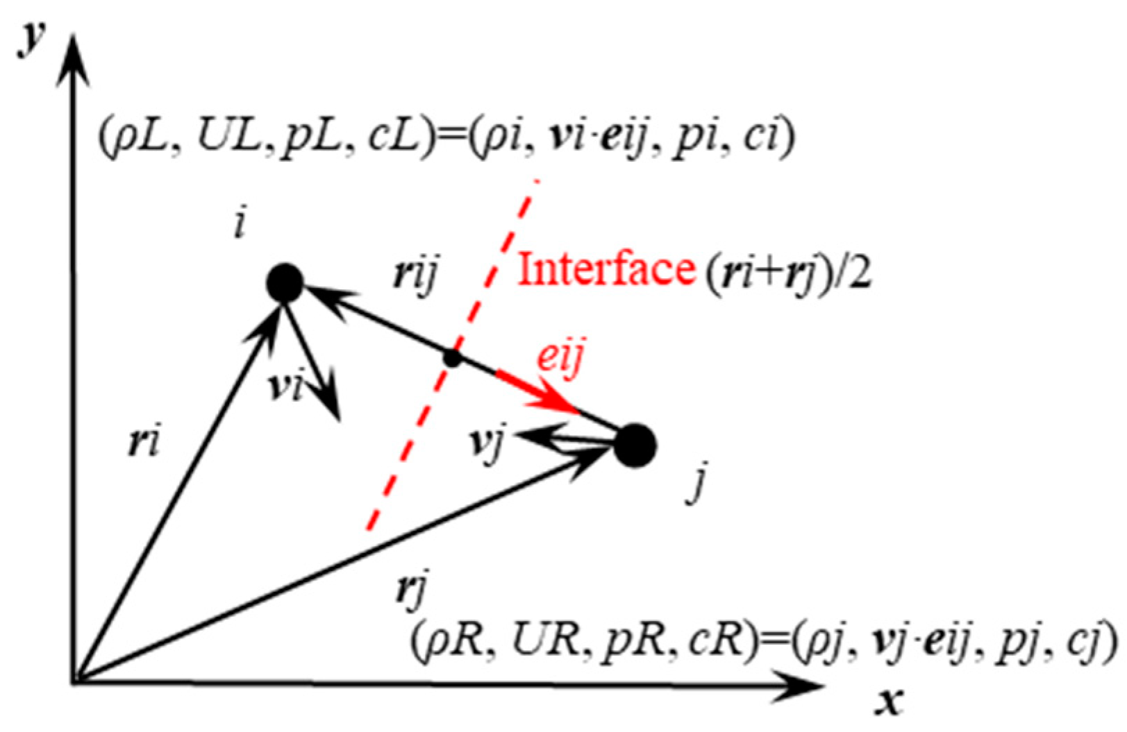
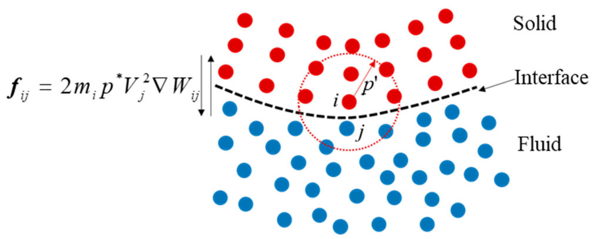
2.3. Riemann-Based Contact Algorithm for Fluids and Solids

This section is divided into subheadings. It should provide a concise and precise description of the experimental results, their interpretation, as well as the experimental conclusions that can be drawn.

When implementing boundary conditions using the virtual particle method in SPH, virtual particles need to be arranged in the initial stage, with their positions either fixed or determined by the fluid particles. This method ensures conservation and facilitates the implementation of slip and non-slip boundary conditions [52]. However, this method is complicated for moving and complex boundaries. Therefore, a modified virtual particle method based on the Riemann model was proposed [53], which can retain the advantages of the virtual particle method and apply to moving and complex boundaries.

This paper implements the contact algorithm based on the following conditions. At a fluid–solid interface, solid particles provide velocity boundary conditions to fluid particles, and fluid particles provide pressure boundary conditions to the solid particles. The solid particles providing velocity boundary conditions to the fluid particles achieve this by including the contribution of the velocities of neighbor solid particles in the discretized continuity equation of the fluid. The fluid particles providing pressure boundary conditions to the solid particles are achieved by defining a virtual pressure, p’, for the solid particles. Equation (12) shows that the virtual pressure is obtained by interpolating the fluid pressure. The first term represents the pressure interpolation of the fluid particles, and the second term is the correction pressure considering hydrostatic pressure [54].

$$p^{\prime }=\frac{{\displaystyle \sum _f{p}_f{W}_{sf}}}{{\displaystyle \sum _f{W}_{sf}}}+\frac{{\displaystyle \sum _f{\rho }_f\left(\mathit{g}-{\mathit{a}}_s\right)\cdot \left({\mathbf{r}}_j-{\mathbf{r}}_f\right)W_{sf}}}{{\displaystyle \sum _f{W}_{sf}}}$$

(12)

where f represents the fluid particles within the supported domain of the solid particle, and a_s is the acceleration of the solid particle.

Then, as shown in Figure 3, the solid particles can be considered pre-arranged virtual particles whose positions are not fixed and are updated based on the solid control equations. The virtual pressure, p′, is assigned to the solid particles. Once the virtual pressure, p′, is obtained, the interaction force between the fluid and solid can be realized through the gradients of fluid pressure and solid virtual pressure.

To improve the stability of the fluid–solid interface, this paper also treats the fluid–solid interface as a discontinuous Riemann model [53]. The contact force between the fluid and solid is modified by solving the intermediate state pressure, p*. Finally, according to the momentum equation, the interaction force between particles i and j can be expressed through Equation (13):

$${\mathit{f}}_{ij}=2m_i{p}^{*}{V}_j^2\nabla W_{ij}$$

(13)

Moreover, to achieve the no-slip boundary condition between the fluid and solid, the velocity, v, of the solid particle can be modified as shown in Equation (14) [54], where j represents the fluid particles within the supported domain of solid particle i, and v_s. is the velocity of the solid itself.

$$\mathit{v}=2{\mathit{v}}_s-{\displaystyle \sum _j\frac{{\mathit{v}}_j{W}_{ij}}{W_{ij}}}$$

(14)

3. Damage Model

Research on metal structures’ deformation and failure response during water entry is necessary. Therefore, this section introduces the damage model in the SPH method. In the TL-SFPM method, the Lagrangian kernel function is based on the initial configuration of the particles. However, when the solid undergoes damage or fracture, losing its continuity, some particles in the supported domain of particle i no longer influence particle i. Therefore, the Lagrangian kernel function is no longer suitable for the current physical model, and an improved algorithm is needed to accurately describe the damage model.

Fortunately, it is known that the Eulerian kernel function in traditional SPH methods describes the interaction between particles based on the current particle configuration. Hence, the following improved algorithm is proposed. When the deformation of solid particle i or its neighbor particles exceeds the damage limitation strain, in the discretized governing equations, the Lagrangian kernel function based on the initial particle configuration is transformed into the Eulerian kernel function based on the current particle configuration. This can capture the distribution of damage around particle i at the present time. The approach fully utilizes the characteristics of the Eulerian kernel function to adaptively adjust the interaction between particles. At this time, the stress term in the governing equations should also be transformed from the first Piola–Kirchhoff stress tensor, P, to the Cauchy stress, σ.

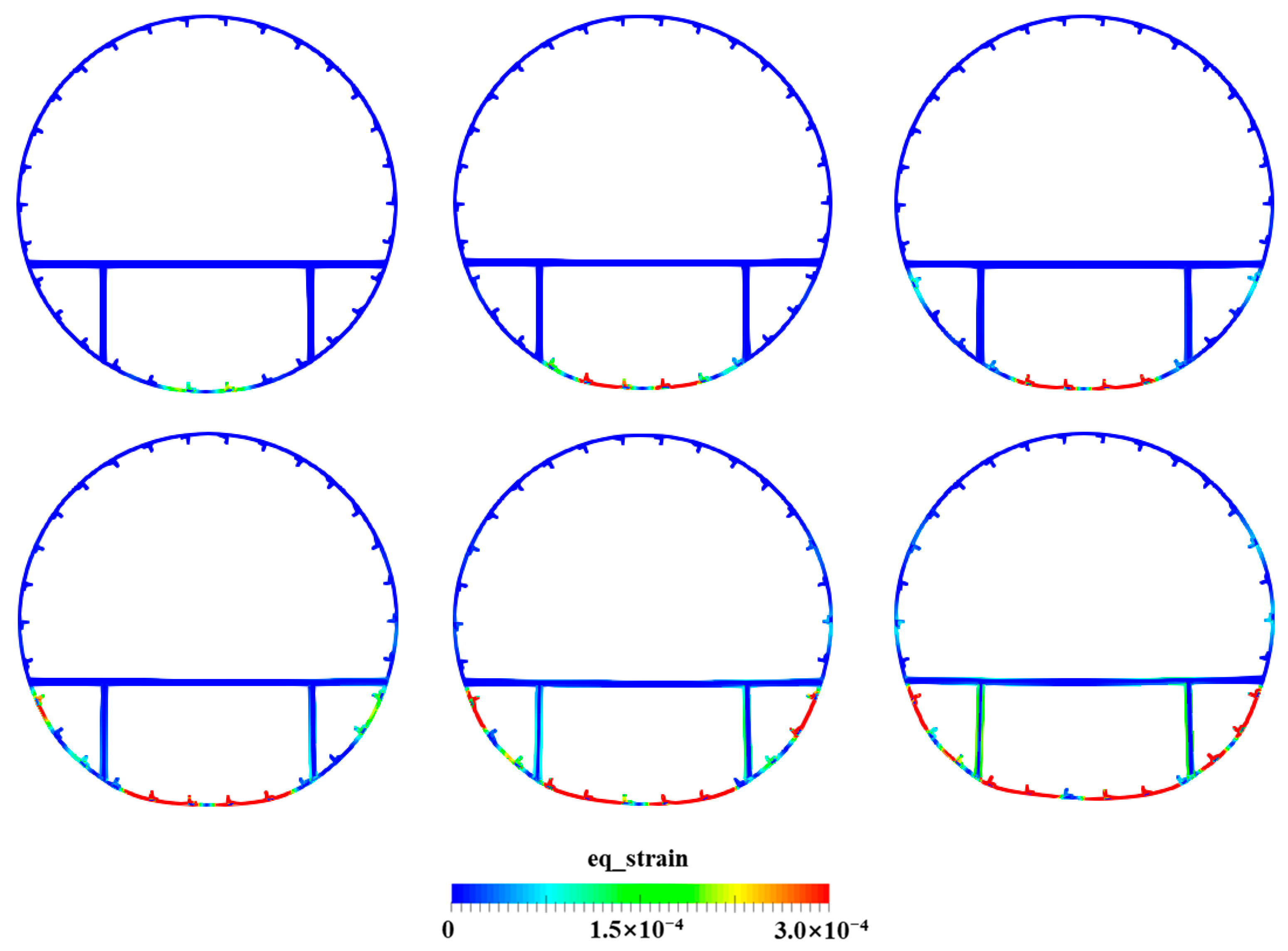
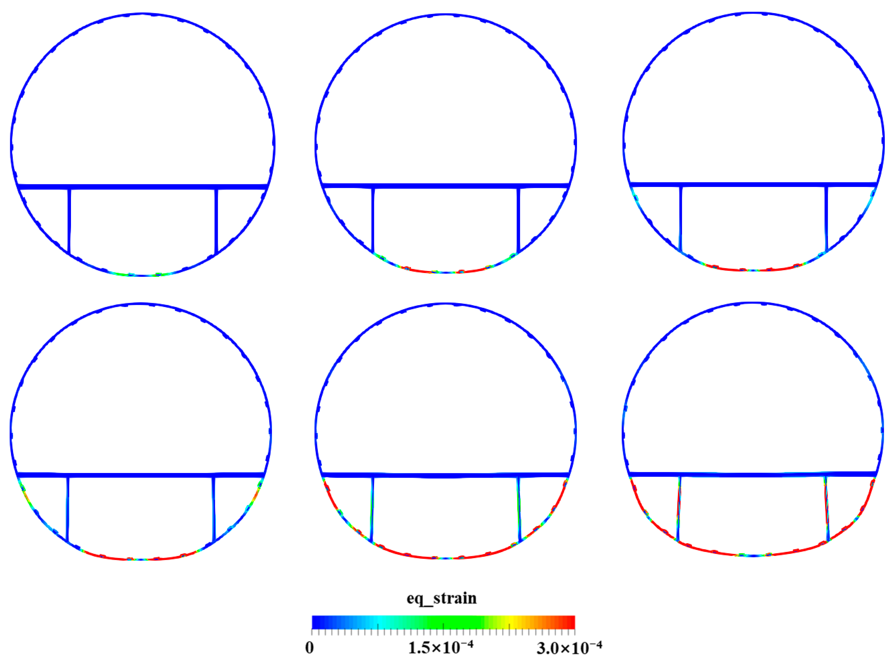
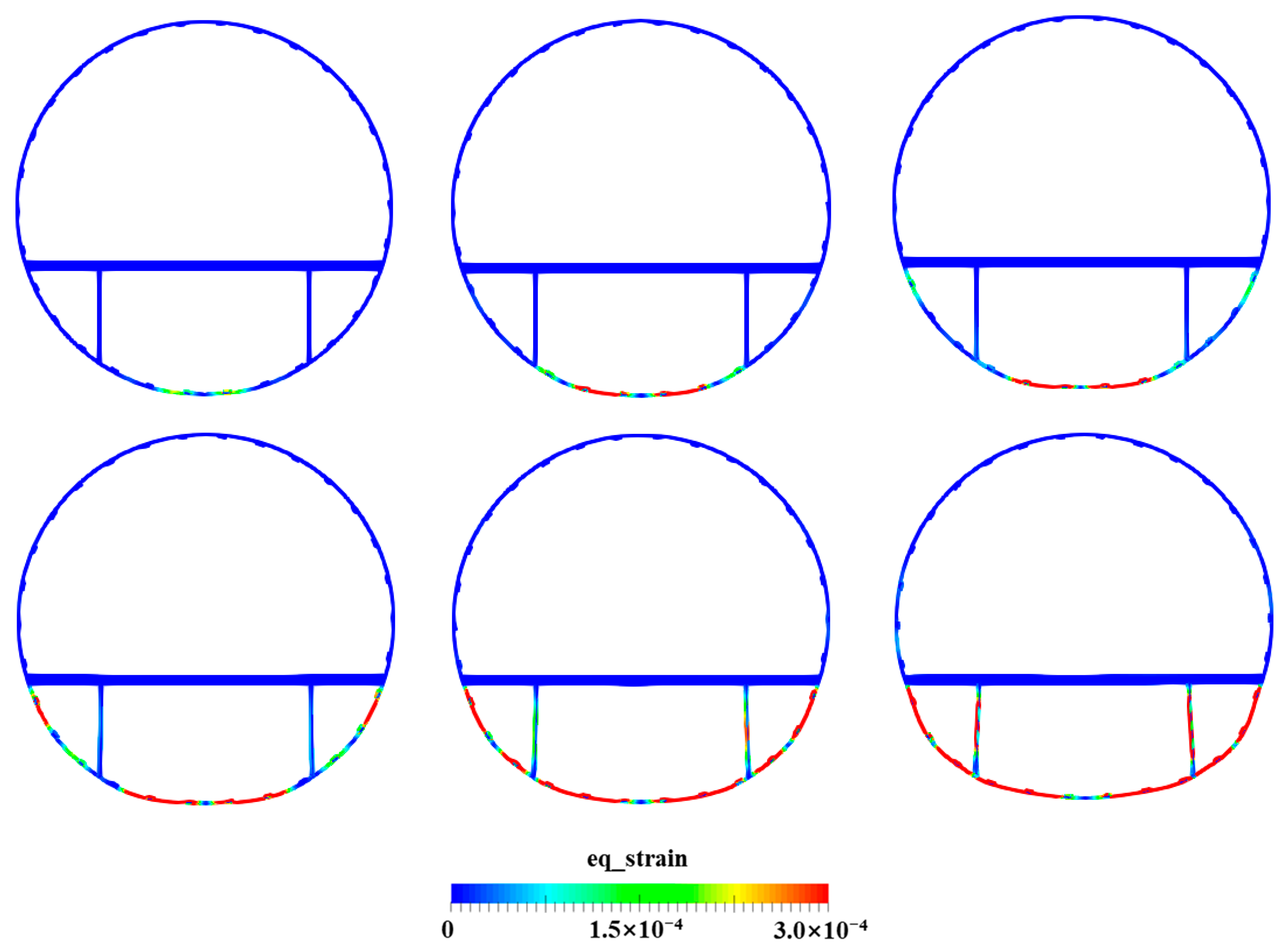
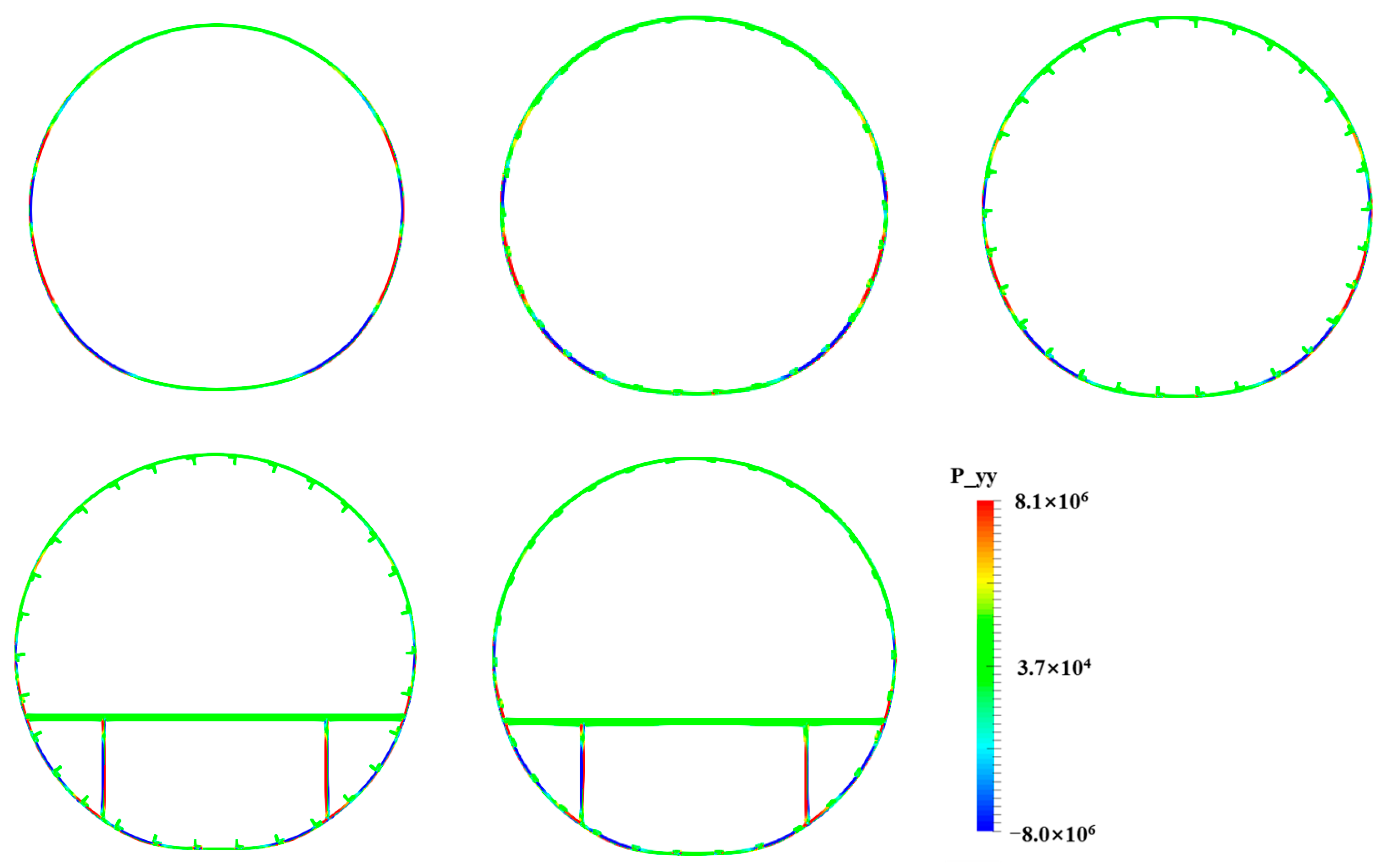
4. Numerical Simulation of Water Entry of a Cylinder Structure

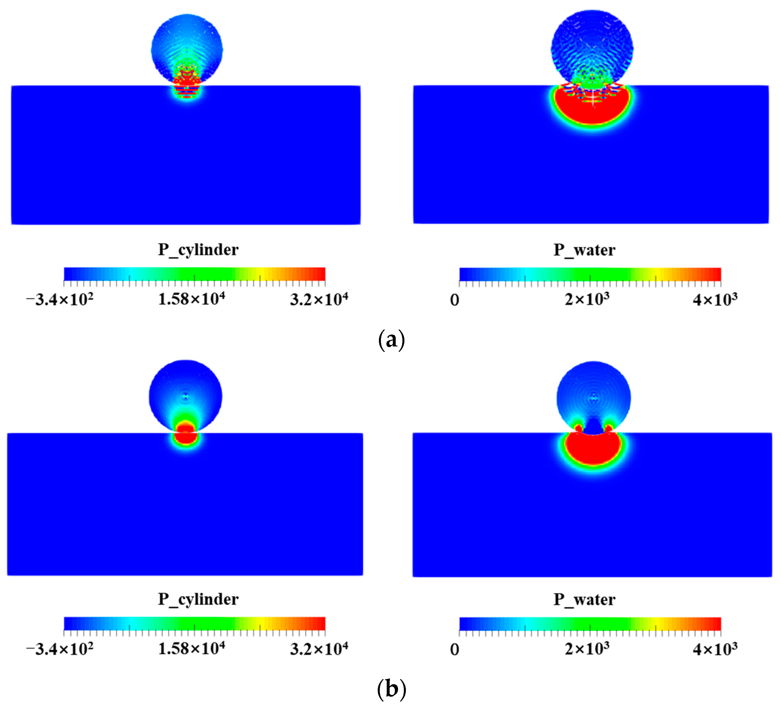
4.1. Validation through Numerical Simulation

To demonstrate the accuracy of the improved SPH model in this paper, this section simulates the water entry of an elastic cylinder structure. The model is consistent with the literature [55]. The water domain has a width of 1 m and a height of 0.4 m, and the radius of the cylinder is 0.1 m. The particle spacing is 0.005 m. The density of the elastic cylinder is 1100 kg/m³, the modulus is 1.2 × 10⁷ N/m², the Poisson’s ratio is 0.4, and the sound speed is 104 m/s. The initial velocity of the cylinder is 2.33 m/s.

Figure 4 displays the isotropic pressure of the elastic cylinder and water obtained via the traditional SPH and improved SPH models. It is observed that the pressure distribution under the traditional SPH is chaotic, while both the pressure of the cylinder and water exhibit a uniform distribution under the improved SPH model. The results show that the improved SPH model can greatly improve tensile instability. From Figure 4b, at the initial water entry stage, the pressure is at its maximum near the interface. As the elastic cylinder continues to enter the water, the isotropic pressure of the elastic cylinder converts into a tensile force, and the pressure of the water propagates downward. Figure 5 provides a comparison of the slamming force experienced by the cylinder obtained from the simulation [55], theory [56], and experiment [57]. The peak value of the slamming force in our simulation is in good agreement with that in the theory and experiment, with an error of 0.024, compared to a peak value error of 0.047 in [55], which validates the computational accuracy of the improved SPH model in this paper. It is also found that, in the theoretical solution and the experiment, the slamming force of the cylinder rises rapidly during water entry, which is faster than that in the simulation. The reason may be that when the slamming force reaches its peak value obtained from the theory and experiment, the depth of the cylinder in the water at this moment is less than the particle spacing of 0.005 m in our simulation, so the simulation cannot be entirely accurate. In [55], it is also indicated that the smaller the spacing is, the faster the slamming force rises.

Next, simulation is performed for the water entry of a skin cylinder. Then, the simulation is conducted for the skin–stringer structure and skin–stringer–floor–column structure. Due to the large physical size of the object and the large number of particles, GPU-accelerated computing is used in this paper. Figure 6 describes the single-GPU parallel flowchart for the SPH method, which shows the main computational part in the GPU, and the CPU only plays the roles of input and output. After initialization, the program transfers the particle information (coordinates, velocity, density, etc.) to the GPU, and the results are transferred back from the device to the host, only reaching the output step.

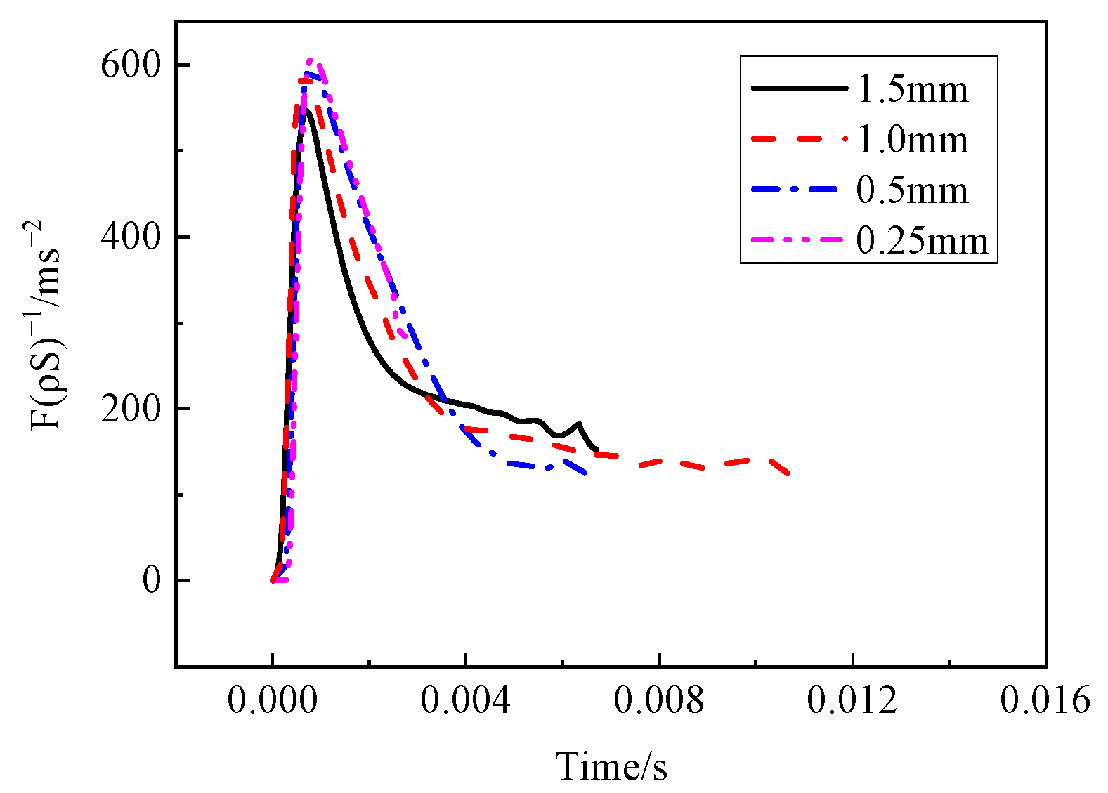
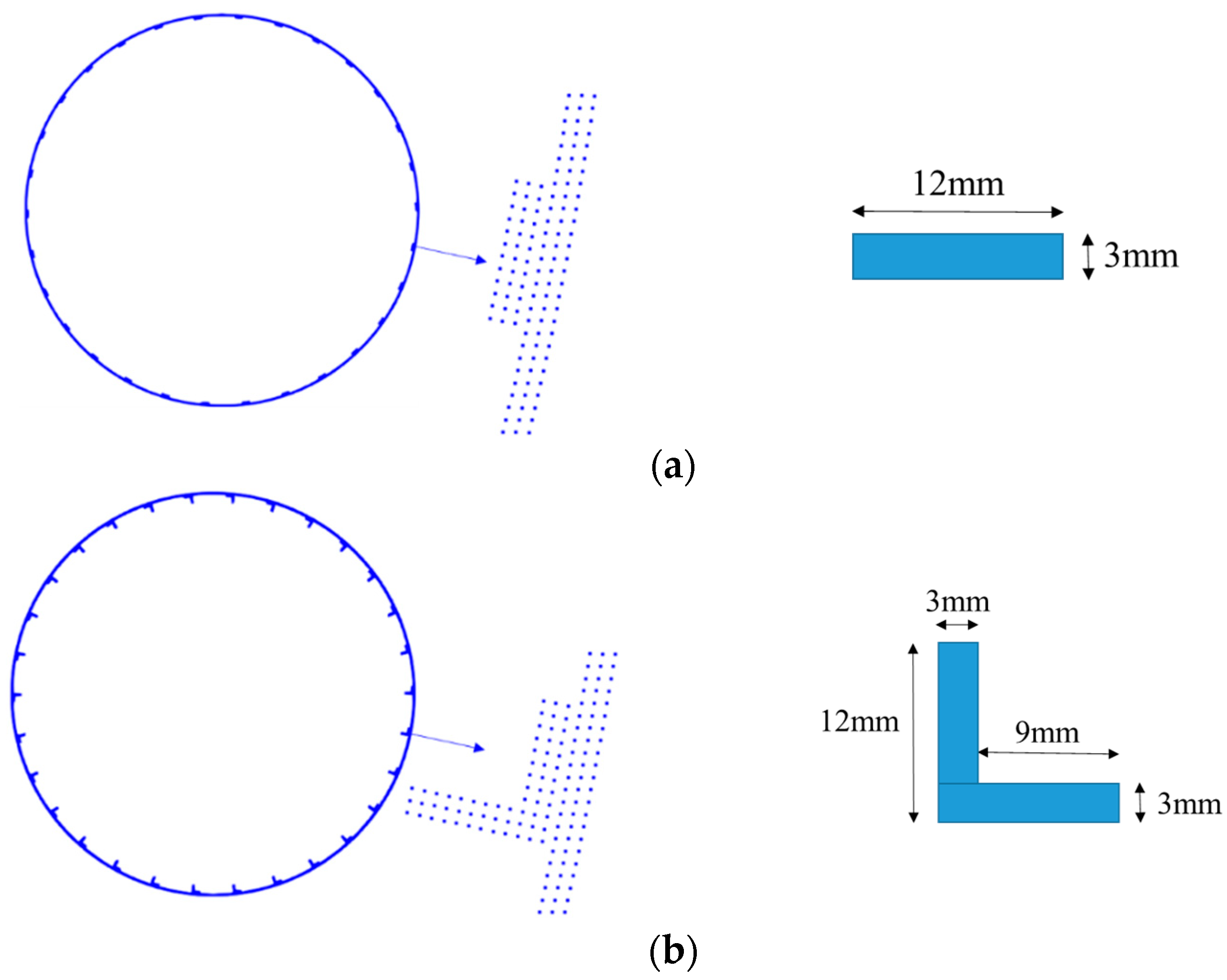
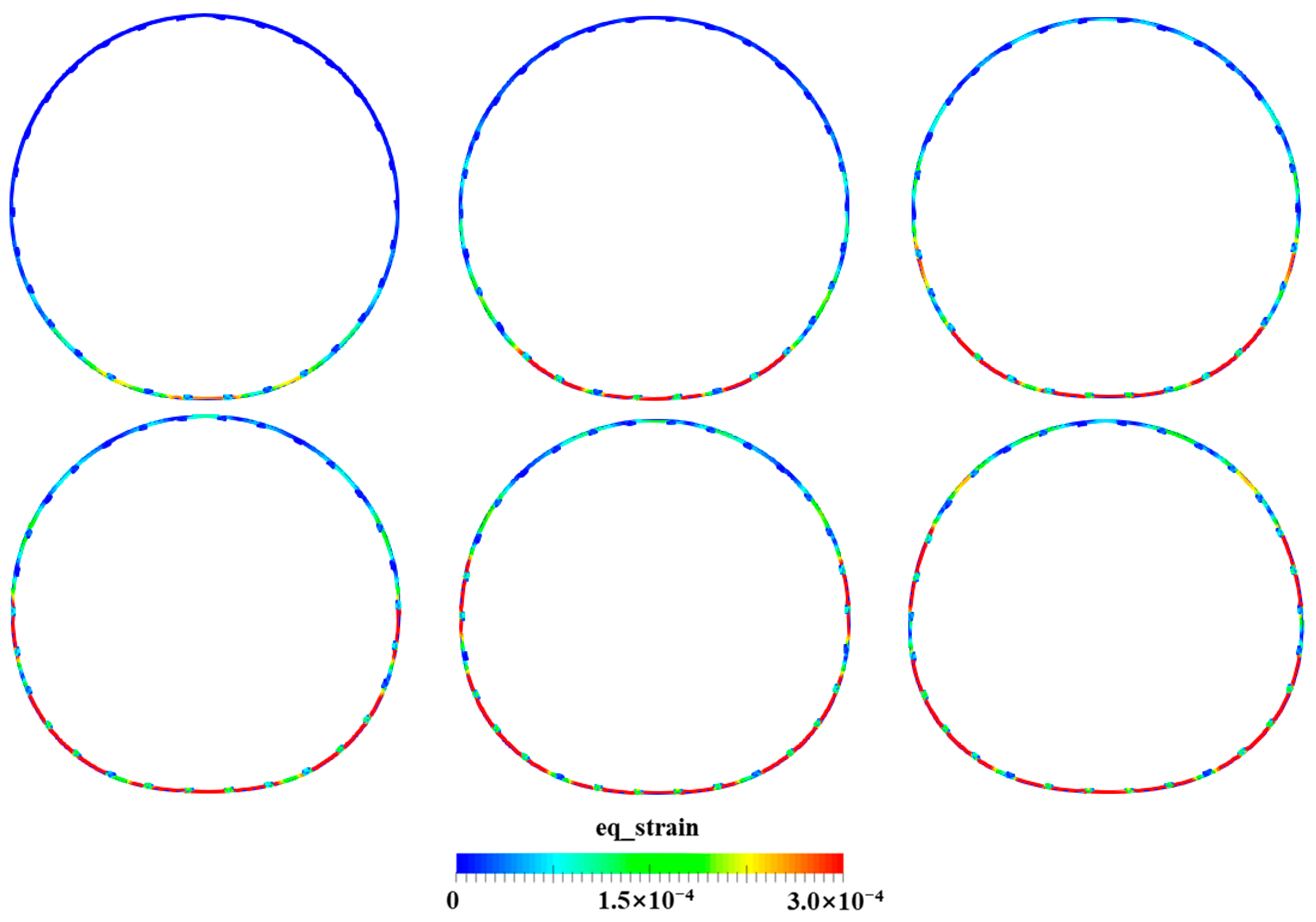
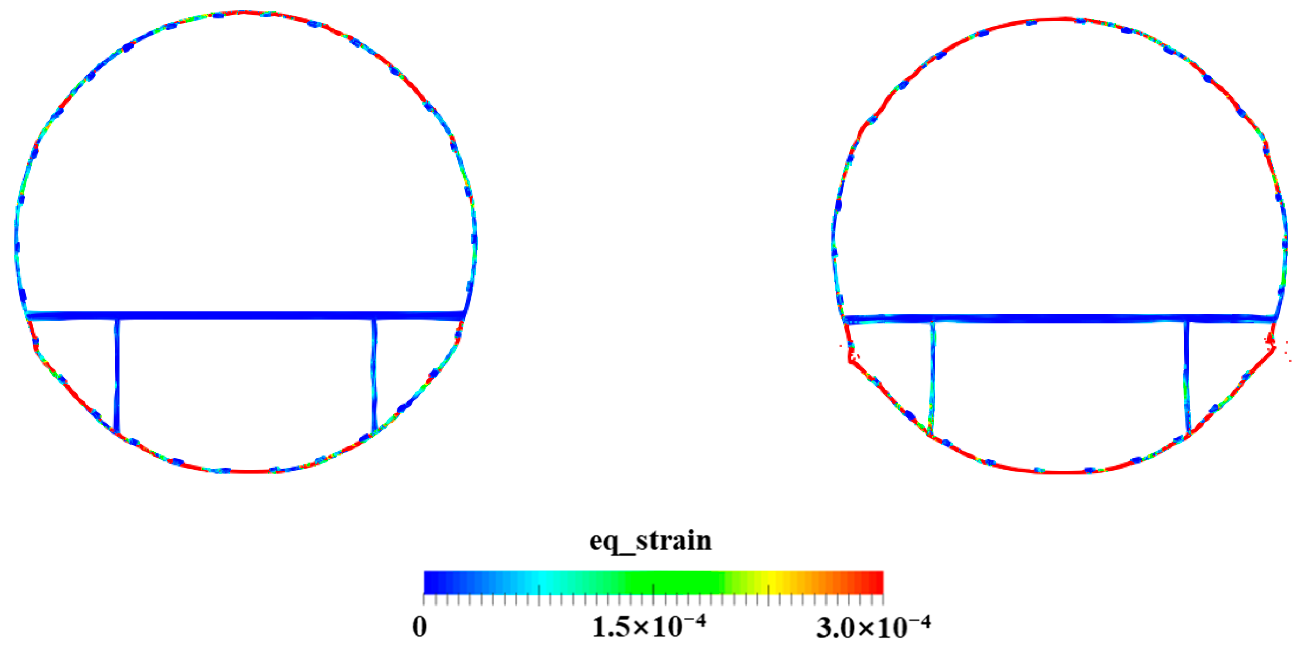
4.2. Water Entry of the Skin Cylinder

The skin cylinder structure has a diameter of 600 mm and a thickness of 3 mm. The material of the cylinder is elastic material with a density of 2700 kg/m³, an elastic modulus of 67.5 GPa, and a Poisson’s ratio of 0.34. The water domain is at a length of 3 m and a height of 2 m. The initial velocity of the cylinder is 5 m/s, representing a free-falling state.

Figure 7 shows the equivalent strain of the cylinder and the pressure of the fluid for the water entry of the cylinder at different times. From the deformation of the cylinder, it can be observed that the bottom of the cylinder undergoes deformation first when it contacts the water’s surface. As the depth of immersion increases, bottom deformation tends to become planar, while the upper part of the cylinder becomes an elliptical shape. It can be seen that the strain originates from the bottom of the cylinder and propagates toward the upper part.

During the deformation of the cylinder, the deformation states of the particles in the innermost and outermost layers are the opposite of each other. The particles in the outermost layer are under compression, the particles in the innermost layer are under tension, and the particles in the middle layer are in a transitional state. The deformation of the particles in the middle layer is minimal.

To further illustrate the convergence of the improved SPH model, Figure 8 provides the variation in the slamming force acting on the cylinder for different particle spacings. The cylinder is arranged with 2, 3, 6, and 12 layers of particles in the thickness direction. As particle spacing decreases, the impact force shows convergent behavior. It is observed that at the moment when the cylinder enters the water, the slamming force rapidly increases to its peak value, followed by a slow decrease. When the slamming force decreases to a value, it exhibits a fluctuating trend. This is due to the continuous downward deformation of the cylinder, resulting in enhanced contact with the water, and the slamming force shows a rising trend.

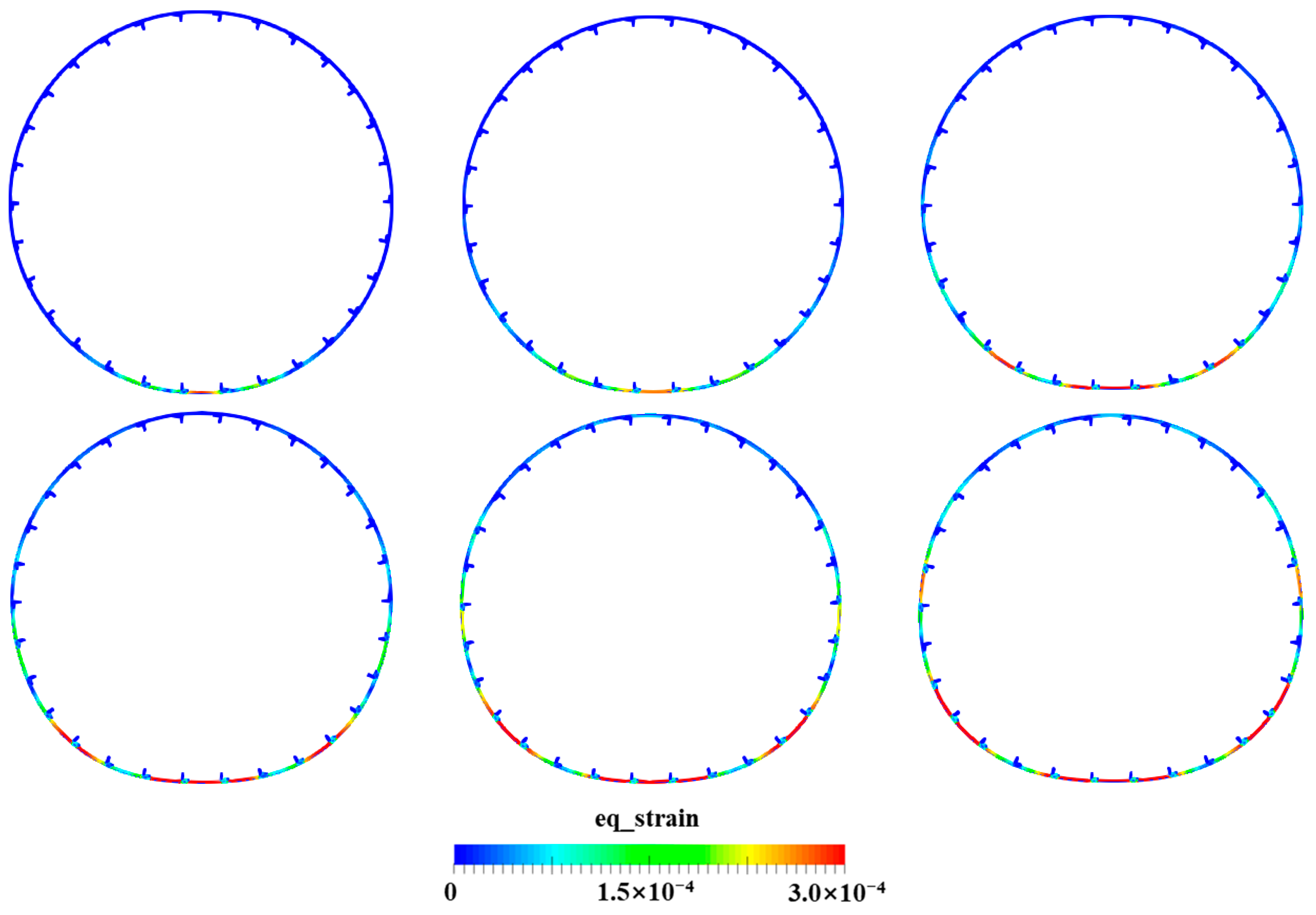
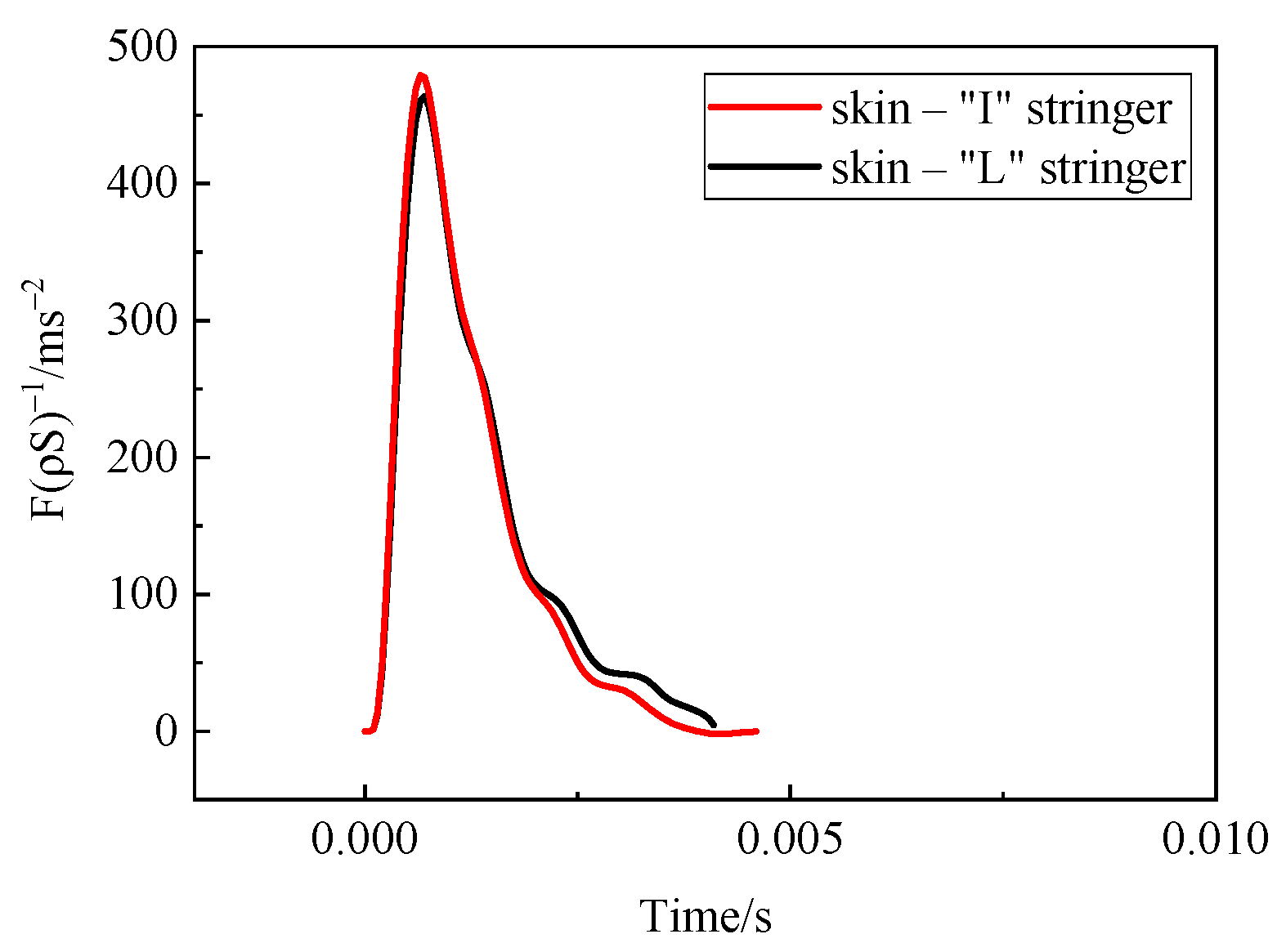
4.3. Water Entry of the Skin–Stringer Cylindrical Structure

Stringers are crucial in resisting damage and transmitting forces within the fuselage. When the skin–stringer cylindrical structure enters water, the deformation of the structure will change. This section discusses the skin–stringer cylindrical structure’s characteristics when it enters water.

Figure 9 shows the shapes of the “I”–type and “L”–type stringers, with 30 stringers uniformly distributed on the cylinder. The dimensions and thickness of the skin remain unchanged, and the material properties and particle spacing are consistent with those in Section 4.2.

Figure 10 shows the equivalent strain at different times for the skin–“I” stringer cylindrical structure. When the structure initially enters the water, deformation primarily occurs at the bottom, becoming increasingly planar in shape, which is similar to the deformation of a pure-skin cylinder. Strain begins to be generated from the bottom of the cylinder and then propagates toward the upper part. The cloud maps show that the strains at the stringer locations are relatively small, indicating that the presence of stringers enhances the structural strength in those locations.

Figure 11 presents the equivalent strain for the skin–“L” stringer cylindrical structure at different times. Similarly, deformation primarily occurs at the bottom in contact with the water and then propagates toward the upper part of the cylinder. Compared to the skin–“I” stringer cylindrical structure, the deformation of the “L” type is smaller, especially toward the top part. Additionally, the strains in the stringer locations are relatively small, indicating that the skin–“L” stringer cylindrical structure provides stronger reinforcement and better maintains the structural shape of the upper skin.

Figure 12 shows the variation in the slamming force over time for the skin–“I” stringer cylindrical structure and skin–“L” stringer cylindrical structure. The slamming force rapidly increases to its peak value. It gradually decreases, but there is a vibration for the slamming force of both “I”-type and “L”-type skin-stringer cylindrical structures during descent. This is because the bottom of the cylinder deforms toward a planar shape, resulting in an increased contact area with the water, leading to an upward trend of the impact force.

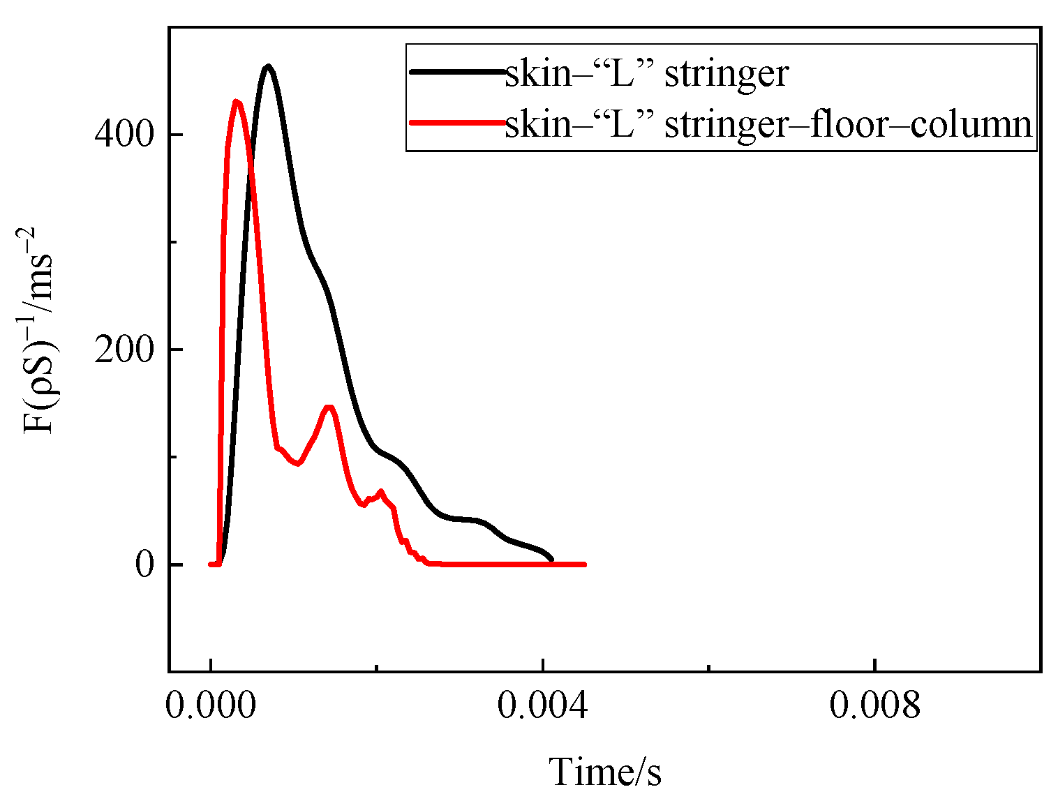
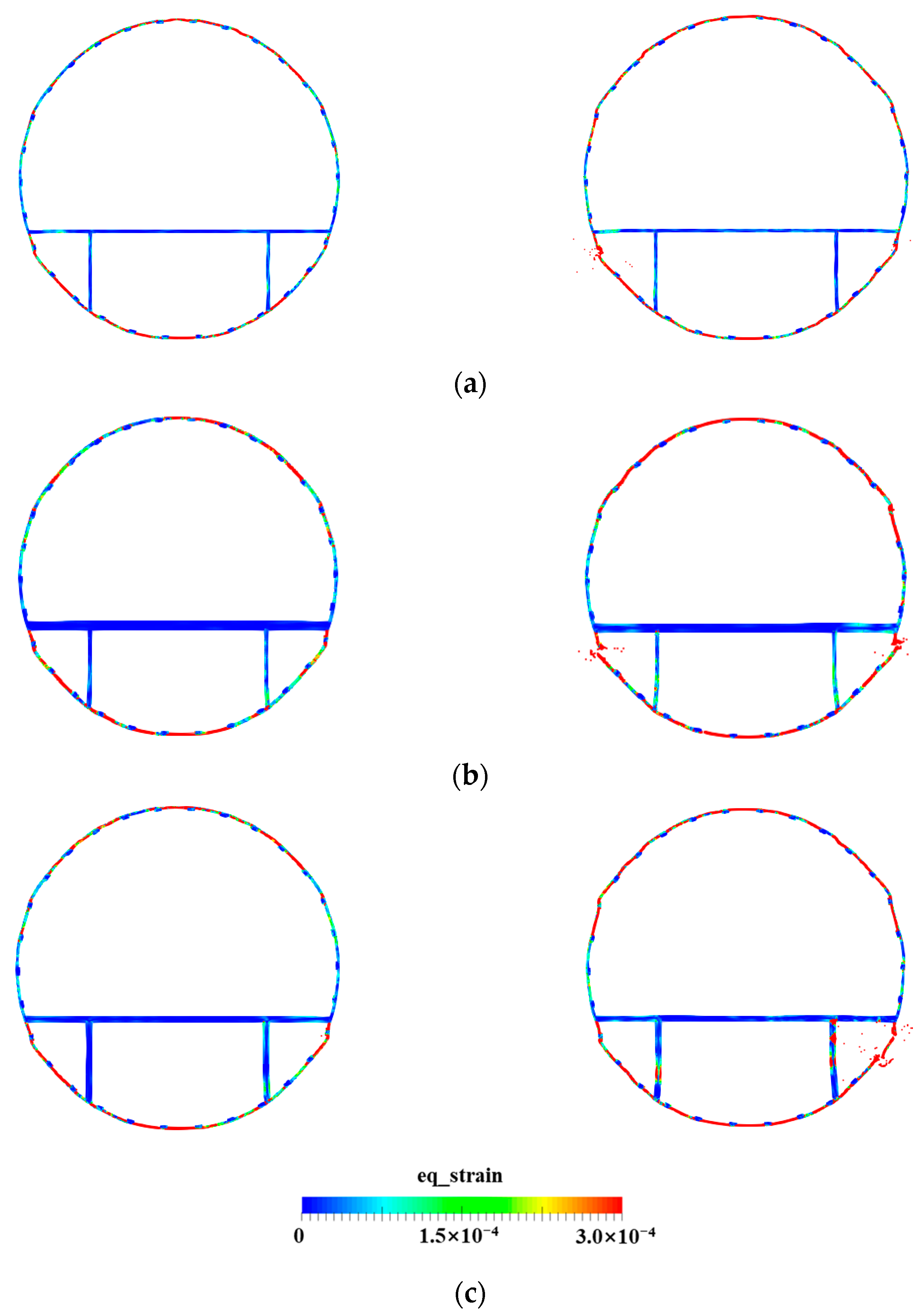
4.4. Water Entry of the Elastic Skin–Stringer–Floor–Column Structure

The floor is an essential component of a commercial aircraft’s fuselage. The floor bears the load of passengers and seats and needs to be connected to the floor’s longitudinal beams, columns, and fuselage frames, making them critical structural elements. Therefore, this section discusses the characteristics of cylindrical structures with floor and columns.

Figure 13 presents the equivalent strain at different times for the skin–“L” stringer–floor–column structure entering the water, with a 10 mm floor thickness. In the initial stage of water entry, the bottom skin starts to deform upwards. As the depth of immersion increases, the deformation of the bottom skin tends toward a planar shape. Due to the support provided by the columns, the column shows a noticeable deformation tendency toward both sides, while the floor exhibits smaller deformation. Throughout the water entry process, the floor and columns support the upper part of the structure, resulting in relatively small deformation and maintaining the shape of the upper space of the structure.

Figure 14 compares the variation in the slamming force over time for the skin–“ L” stringer structures with and without floor and columns. After the structure touches the water, the slamming force rapidly increases to its peak value and gradually decreases. It can be observed that the structure with floor and columns has a higher weight, leading to a faster increase in the slamming force but with a smaller peak value. During descent, the impact force exhibits fluctuations and a trend of increase, which is caused by the deformation of the bottom skin and a larger area of contact with the water.

Next, the influence of floor thickness on structural deformation is explained. Figure 15 and Figure 16 show the equivalent strain at different times for the structure with a floor thickness of 5 mm and 15 mm, respectively. When the floor thickness decreases, the differences in deformation are minimal at the bottom skin and columns. The influence can be observed on the above floor. A decreased floor thickness reduces the energy absorption from the lower part, resulting in more considerable deformation in the upper skin. Conversely, when floor thickness increases, the differences in deformation also are minimal at the bottom skin, and the deformation of the columns decreases, with almost no deformation observed in the upper skin.

It can be concluded that floor thickness has a small influence on the deformation of the bottom skin, but significantly affects the deformation of the columns and upper skin. The floor is an important component for supporting the shape of the upper structure, and selecting an appropriate floor thickness is crucial for a structurally safe design.

Figure 17 compares the variation in the slamming force over time for structures with a floor of thickness 5 mm, 10 mm, and 15 mm. The three curves exhibit almost identical trends. The structure with a 15 mm floor thickness shows the smallest peak value. The fluctuations in the slamming force during the descent phase are consistent.

Figure 18 shows that there is an equivalent strain at different times for the structure if the diameter of the columns is increased. It can be observed that increasing the column diameter effectively reduces the deformation of the columns, floor, and upper skin, providing beneficial protection for the overall structure.

By changing the stringers from the “L” type to the “I” type and further studying the water entry behavior of the skin–“I” stringer–floor–column structure (Figure 19, Figure 20, Figure 21, Figure 22, Figure 23 and Figure 24), it is found that the “I” type stringer structure exhibits similar changes in deformation and slamming force before and after the addition of floor and columns. The influence of floor thickness is also consistent. It can be concluded that floor thickness has a small impact on the deformation of the structure below the floor. Similarly, a thicker floor results in a smaller deformation of the upper skin and columns, better maintaining the shape of the upper space. A larger column diameter leads to smaller deformation in the floor, columns, and upper skin.

Next, the effects of structural geometry on the stress distribution are discussed. Figure 25 compares the first Piola–Kirchhoff stress in the yy direction that is consistent with the direction of water entry at the moment along the skin cylinder, the that in the skin–stringer cylindrical structure, and that in the skin–stringer–floor–column structure. It is found that the stress distribution is similar between the skin cylinder and the skin–stringer cylindrical structure. However, there is a stress concentration phenomenon near the stringer for the skin–stringer cylindrical structure, and the stress at the top of the skin is smaller than that of the skin cylinder. The stress is mainly distributed under the floor for the skin–stringer–floor–column structure. Greater stress appears in the vertical column, reflecting that the floor and column can protect the upper part of the structure. Moreover, the stress concentration phenomenon near the stringer also can be observed.

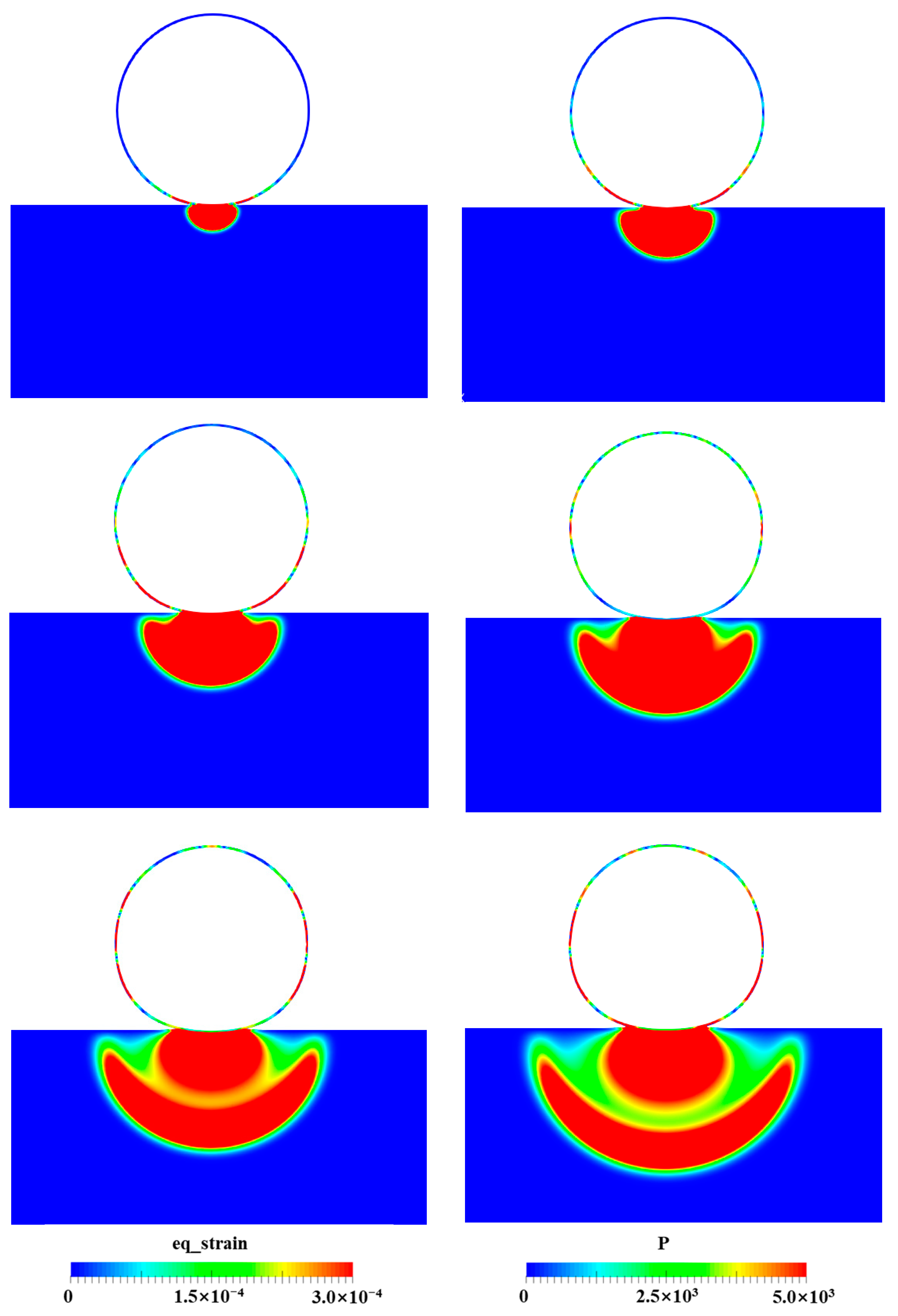
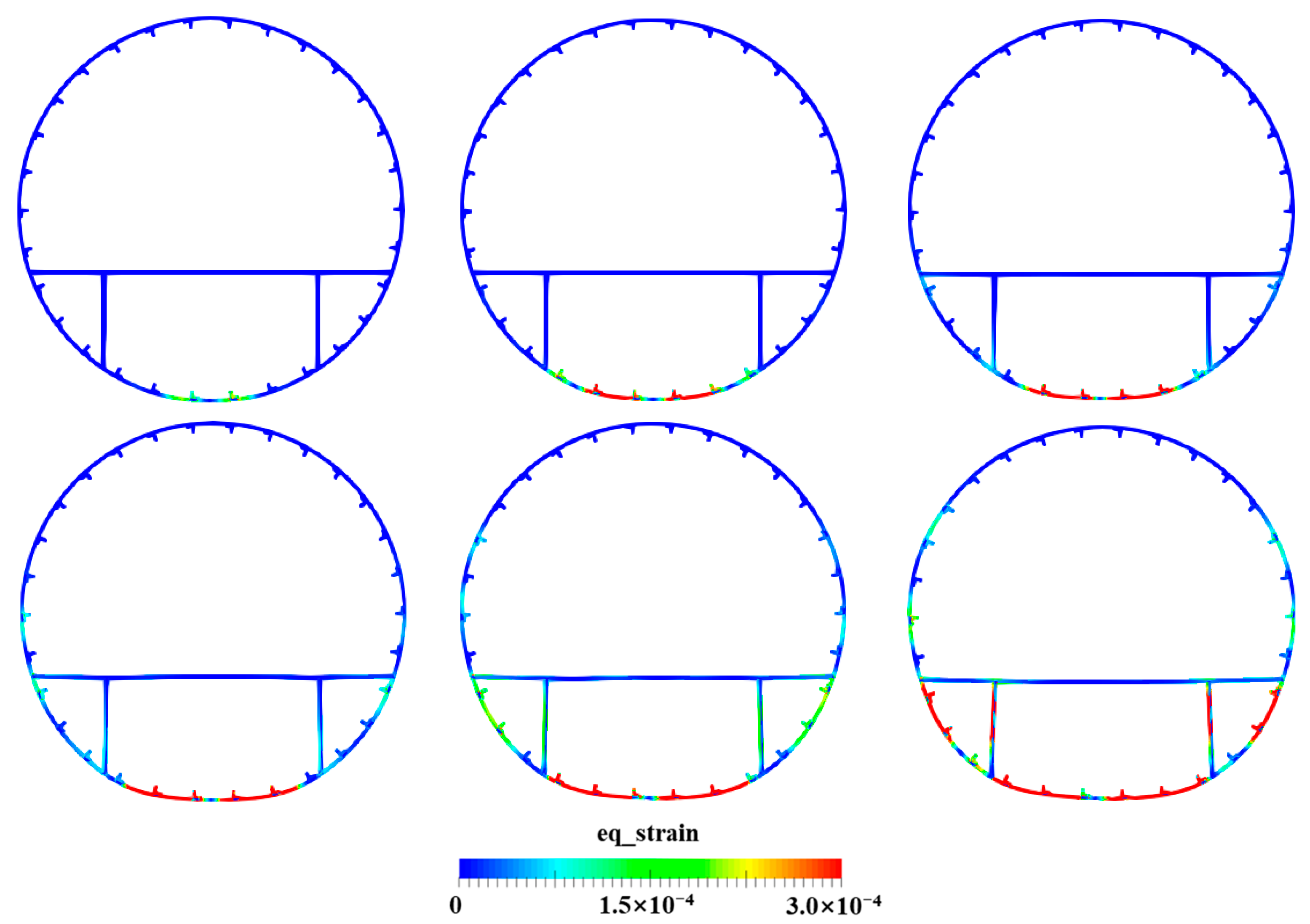
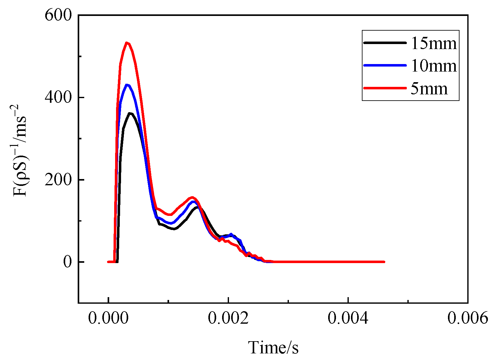
4.5. Water Entry of the Elastic–Plastic Skin–Stringer–Floor–Column Structure

In previous studies, the objective has been to analyze the elastic behavior of the skin–stringer–floor–column structure during water entry. The material of the structure is assumed to be elastic. To further investigate the deformation and failure response of the metal structures, this section extends the structural material to metal elastic–plastic materials.

The constitutive model for the elastic–plastic material is the Johnson–Cook yield model [58];

Table 1. Constitutive parameters for elastic–plastic material.

Physical Quantity	Value	Physical Quantity	Value
Density, ρ, kg/m3	2700	Hardening coefficient, B, MPa	426
Sound speed, Cs, m/s	5000	Strain hardening index, n	0.34
Poisson ratio, ν	0.34	Strain rate coefficient, C	0.015
E, GPa	67.5	Thermal softening coefficient, m	1.0
Static yield strength, A, MPa	265	Specific heat, Cv, J/kgK	875

provides the constitutive parameters for elastic–plastic material, and Figure 26 shows the equivalent strain of the skin–‘‘I’’ stringer–floor–column structure at different times. It can be observed that compared to an elastic structure, an elastic–plastic structure exhibits significant deformation in the upper and lower parts of the skin, and small deformation in the floor and columns. The upper part is still able to maintain its basic shape. The final failure occurs in the lower skin near the floor, where stress concentration is observed.

By changing the floor thickness and the column diameter, it can be observed from Figure 27 that the locations of structural failure are all in the lower skin near the floor, indicating that this area is vulnerable during the water entry process and needs further reinforcement.

5. Conclusions

This paper addresses the fluid–solid coupling problem of the water entry of the fuselage structure and presents an improved smoothed particle hydrodynamics (SPH) model, which includes the low-dissipation GSPH method, the total Lagrangian SFPM method, and the Riemann-based contact algorithm. The rationality of the improved SPH model is demonstrated through the simulation of the water entry of an elastic cylinder via comparison with the theoretical and experimental results.

Furthermore, the dynamic characteristics of the skin cylindrical structure, skin–stringer cylindrical structure, and skin–stringer–floor–column structure during water entry are studied. A comparative analysis of the strain distribution and slamming force reveals that in the case of the skin cylindrical structure, deformation primarily occurs at the bottom initially. With an increasing depth of water entry, the bottom’s deformation causes it to transition toward a planar shape, and the top of the cylinder becomes pointed, ultimately deforming into an elliptical shape. The deformation pattern of the skin–stringer cylindrical structure is similar, but strains in the stringer are smaller. In the case of the skin–stringer–floor–column structure, the columns exhibit notable deformation due to the upper structure’s column support, while the floor undergoes small deformation. Throughout the water entry process, the portion of the structure above the floor remains relatively less deformed, thus better maintaining the upper spatial shape. The trend of the slamming force for the three structures is similar between them. After contacting the water surface, the impact force rapidly rises to a peak and then gradually decreases. In the decreasing phase, the impact force exhibits oscillations, which occur as the bottom of the structure transforms into a plane, resulting in an increased contact area between the structure and water, consequently enhancing the slamming force.

The influence of floor thickness and column diameter is also discussed. It is observed that floor thickness has a small effect on the bottom skin’s deformation but significantly affects the columns and upper skin deformation. The floor serves as a crucial component supporting the shape of the upper structure, making a reasonable choice of floor thickness vital for structurally safe design. Increasing the column diameter effectively reduces the column, floor, and upper skin deformation, thus playing a favorable role in protecting the overall structure.

Based on the damage model, a study is conducted on the water entry of a metallic elastic–plastic skin–stringer–floor–column structure, analyzing the positions of plastic deformation and failure. Compared to elastic structures, greater deformation occurs in the skin’s upper and lower portions in plastic structures, but the upper part still maintains its basic shape. Ultimately, failure occurs in the bottom skin section close to the floor, where stress concentration appears.

In this paper, the material of the fuselage is aluminum, which is a commonly used metal material in aircraft. The most recent airplanes increasingly use carbon fiber composite material. Hence, we need to further study the water entry characteristics of the composite materials, which is our future work.

References

1. Siemann, M.H. Numerical and Experimental Investigation of the Structural Behavior during Aircraft Emergency Landing on Water. Ph.D. Thesis, University of Stuttgart, Stuttgart, Germany, 2016. [Google Scholar]
2. Climent, H.; Benítez, L.; Rosich, F.; Rueda, F.; Pentecôte, N. Aircraft ditching numerical simulation. In Proceedings of the 25th International Congress of the Aeronautical Sciences, Hamburg, Germany, 3–8 September 2006. [Google Scholar]
3. Zheng, Y.; Qu, Q.; Liu, P.; Wen, X.; Zhang, Z. Numerical analysis of the porpoising motion of a blended wing body aircraft during ditching. Aerosp. Sci. Technol. 2021, 119, 107131. [Google Scholar] [CrossRef]
4. Streckwall, H.; Lindenau, O.; Bensch, L. Aircraft ditching: A free surface/free motion problem. Arch. Civ. Mech. Eng. 2007, 7, 177–190. [Google Scholar] [CrossRef]
5. Seddon, C.; Moatamedi, M. Review of water entry with applications to aerospace structures. Int. J. Impact Eng. 2006, 32, 1045–1067. [Google Scholar] [CrossRef]
6. Pentecote, N. Validation of the PAM-CRASH Code for the Simulation of the Impact on Water; DLR–IB 435.2003/3; Institute of Transport Research: New York, NY, USA, 2003. [Google Scholar]
7. Pentecote, N.; Vigliotti, A. Crashworthiness of helicopters on water: Test and simulation of a full-scale WG30 impacting on water. Int. J. Crashworthiness 2003, 8, 559–572. [Google Scholar] [CrossRef]
8. Von Karman, T.H. The Impact on Seaplane Floats During Landing, National Advisory Committee for Aeronautics; NACA-TN-321; 93R10464; National Advisory Committee for Aeronautics: Boston, MA, USA, 1929. [Google Scholar]
9. Wagner, H. Phenomena Associated with Impact and Gliding on a Liquid Surface. NACA Transl. 1932, 93R10464. [Google Scholar]
10. Farhat, G. Analytical method for the ditching analysis of an airborne vehicle. J. Aircr. 1989, 27, 312–319. [Google Scholar]
11. Pentecôte, N.; Kohlgrüber, D. Full-scale simulation of aircraft impacting on water. In Proceedings of the International Crashworthiness Conference, San Francisco, CA, USA, 14–16 July 2004. [Google Scholar]
12. Hua, C.; Fang, C.; Cheng, J. Simulation of fluid–solid interaction on water ditching of an airplane by ALE method. J. Hydrodyn. 2011, 23, 637–642. [Google Scholar] [CrossRef]
13. Ortiz, R.; Portemont, G.; Charles, J.L.; Sobry, J.F. Assessment of Explicit FE Capabilities for Full Scale Coupled Fluid/Structure Aircraft Ditching Simulations. In Proceedings of the 23rd International Congress of the Aeronautical Sciences, Toronto, ON, Canada, 8–13 September 2002; pp. 8–13. [Google Scholar]
14. Qu, Q.; Hu, M.; Guo, H.; Liu, P.; Agarwal, R.K. Study of ditching characteristics of transport aircraft by global moving mesh method. J. Aircr. 2015, 52, 1550–1558. [Google Scholar] [CrossRef]
15. Woodgate, M.A.; Barakos, N.G.; Scrase, N.; Neville, T. Simulation of helicopter ditching using smoothed particle hydrodynamics. Aerosp. Sci. Technol. 2019, 85, 277–292. [Google Scholar] [CrossRef]
16. Barreiro, A.; Crespo, A.J.C.; Dominguez, J.M.; Gomez-Gesteira, M. Smoothed particle hydrodynamics for coastal engineering problems. Comput. Struct. 2013, 120, 96–106. [Google Scholar] [CrossRef]
17. Hu, X.Y.; Adams, N.A. A multi-phase SPH method for macroscopic and mesoscopic flows. J. Comput. Phys. 2006, 213, 844–861. [Google Scholar] [CrossRef]
18. Gray, J.P.; Monaghan, J.J.; Swift, R.P. SPH elastic dynamics. Comput. Methods Appl. Mech. Eng. 2001, 190, 6641–6662. [Google Scholar] [CrossRef]
19. Zhang, X.; Xu, F.; Yang, Y.; Ren, X.; Wang, L.; Yang, Q.; Xu, C. An improved SPH scheme for the 3D FEI (Fluid-Elastomer Interaction) problem of aircraft tire spray. Eng. Anal. Bound. Elem. 2023, 153, 295–304. [Google Scholar]
20. Zhang, T.; Li, Y.; Li, C.; Sun, S. Effect of salinity on oil production: Review on low salinity waterflooding mechanisms and exploratory study on pipeline scaling. Oil Gas Sci. Technol. Rev. IFP Energ. Nouv. 2020, 75, 50. [Google Scholar] [CrossRef]
21. Liu, J.; Zhang, T.; Sun, S. Study of the Imbibition Phenomenon in Porous Media by the Smoothed Particle Hydrodynamic (SPH) Method. Entropy 2022, 24, 1212. [Google Scholar] [CrossRef]
22. Zhu, C.; Huang, Y.; Zhang, L. SPH-based simulation of flow process of a landslide at Hongao landfill in China. Nat. Hazards 2018, 93, 1113–1126. [Google Scholar] [CrossRef]
23. Zheng, H.; Bin, S.; Yange, L. Numerical simulation of debris-flow behavior based on the SPH method incorporating the Herschel-Bulkley-Papanastasiou rheology model. Eng. Geol. 2019, 255, 25–36. [Google Scholar]
24. Monaghan, J.J. SPH without a Tensile Instability. J. Comput. Phys. 2000, 159, 290–311. [Google Scholar] [CrossRef]
25. Swegle, J.W.; Hicks, D.L.; Attaways, S.W. Smoothed Particle Hydrodynamics Stability Analysis. J. Comput. Phys. 1995, 116, 123–134. [Google Scholar] [CrossRef]
26. Zhu, C.; Chen, Z.; Huang, Y. Coupled moving particle simulation–finite-element method analysis of fluid–structure interaction in geodisasters. Int. J. Geomech. 2021, 21, 6. [Google Scholar] [CrossRef]
27. Huang, Y.; Zhu, C. Numerical analysis of tsunami–structure interaction using a modified MPS method. Nat. Hazards 2015, 75, 2847–2862. [Google Scholar] [CrossRef]
28. Huang, Y.; Zhu, C. Simulation of flow slides in municipal solid waste dumps using a modified MPS method. Nat. Hazards 2014, 74, 491–508. [Google Scholar] [CrossRef]
29. Otto, R.; Gilberto, D.; Jaime, K. Local Consistency of Smoothed Particle Hydrodynamics (SPH) in the Context of Measure Theory. Front. Appl. Math. Stat. 2022, 8, 907604. [Google Scholar]
30. Evers, J.H.M.; Zisis, I.A.; van der Linden, B.J.; Duong, M.H. From continuum mechanics to SPH particle systems and back: Systematic derivation and convergence. J. Appl. Math. Mech. 2018, 98, 106–133. [Google Scholar] [CrossRef]
31. Sigalotti, L.D.G.; Rendón, O.; Klapp, J.; Vargas, C.A.; Cruz, F. A new insight into the consistency of the SPH interpolation formula. Appl. Math. Comput. 2019, 356, 50–73. [Google Scholar] [CrossRef]
32. Quinlan, N.; Basa, M.; Lastiwka, M. Truncation error in mesh-free particle methods. Int. J. Numer. Methods Eng. 2006, 66, 2064–2085. [Google Scholar] [CrossRef]
33. Vaughan, G.L.; Healy, T.R.; Bryan, K.R.; Sneyd, A.D.; Gorman, R.M. Completeness, conservation and error in SPH for fluids. Int. J. Numer. Methods Fluids 2008, 56, 37–62. [Google Scholar] [CrossRef]
34. Read, J.I.; Hayfield, T.; Agertz, O. Resolving mixing in smoothed particle hydrodynamics. Mon. Not. R. Astron. Soc. 2010, 405, 1513–1530. [Google Scholar] [CrossRef]
35. Qirong, Z.; Lars, H.; Yuexing, L. Numerical Convergence in Smoothed Particle Hydrodynamics. Cosmol. Nongalactic Astrophys. 2015, 800, 6. [Google Scholar]
36. Leonardo, D.G.S.; Jaime, K.; Moncho, G.G. The mathematics of smoothed particle hydrodynamics (SPH) consistency. Front. Appl. Math. Stat. 2021, 7, 797455. [Google Scholar]
37. Chen, J.K.; Beraun, J.E. A generalized smoothed particle hydrodynamics method for nonlinear dynamic problem. Comput. Methods Appl. Mech. Eng. 2000, 190, 225–239. [Google Scholar] [CrossRef]
38. Liu, M.B.; Liu, G.R. Restoring particle consistency in smoothed particle hydrodynamics. Appl. Numer. Math. 2006, 56, 19–36. [Google Scholar] [CrossRef]
39. Monaghan, J.J.; Gingold, R.A. Shock simulation by the particle method SPH. J. Comput. Phys. 1983, 52, 374–389. [Google Scholar] [CrossRef]
40. Bouscasse, B.; Colagrossi, A.; Marrone, S. Nonlinear water wave interaction with floating bodies in SPH. J. Fluids Struct. 2013, 42, 112–129. [Google Scholar] [CrossRef]
41. Sun, P.N.; Colagrossi, A.; Marrone, S. The δplus-SPH model: Simple procedures for a further improvement of the SPH scheme. Comput. Methods Appl. Mech. Eng. 2017, 315, 25–49. [Google Scholar] [CrossRef]
42. Zhang, C.; Hu, X.Y.; Adams, N.A. A weakly compressible SPH method based on a low-dissipation Riemann solver. J. Comput. Phys. 2017, 335, 605–620. [Google Scholar] [CrossRef]
43. Leonardo, D.G.S.; Hender, L. Adaptive kernel estimation and SPH tensile instability. Comput. Math. Appl. 2008, 55, 23–50. [Google Scholar]
44. Dyka, C.T.; Andles, P.W.; Ingel, R.P. Stress points for tension instability in SPH. Int. J. Numer. Methods Eng. 1997, 40, 2325–2341. [Google Scholar] [CrossRef]
45. Sugiura, K.; Inutsuka, S. An extension of Godunov SPH II: Application to elastic dynamics. J. Comput. Phys. 2017, 333, 78–103. [Google Scholar] [CrossRef]
46. Belytschko, T.; Xiao, S. Stability analysis of particle methods with corrected derivatives. Comput. Math. Appl. 2002, 43, 329–350. [Google Scholar] [CrossRef]
47. Belytschko, T.; Guo, Y.; Liu, W.K. A unified stability analysis of meshless particle methods. Int. J. Numer. Methods Eng. 2000, 48, 1359–1400. [Google Scholar] [CrossRef]
48. Chen, C.; Zhang, A.; Chen, J. SPH simulations of water entry problems using an improved boundary treatment. Ocean Eng. 2021, 238, 109679. [Google Scholar] [CrossRef]
49. Monaghan, J.J. Smoothed Particle Hydrodynamics and Its Diverse Applications. Annu. Rev. Fluid Mech. 2012, 44, 323–346. [Google Scholar] [CrossRef]
50. Wang, L.; Xu, F.; Yang, Y. Improvement of the tensile instability in SPH scheme for the FEI (Fluid-Elastomer Interaction) problem. Eng. Anal. Bound. Elem. 2019, 106, 116–125. [Google Scholar] [CrossRef]
51. Wang, L.; Xu, F.; Yang, Y. An improved total Lagrangian SPH method for modeling solid deformation and damage. Eng. Anal. Bound. Elem. 2021, 133, 286–302. [Google Scholar] [CrossRef]
52. Zhang, C.; Yujie, Z.; Dong, W. Smoothed particle method for fluid-structure interaction. Sci. Sin. Physica Mech. Astron. 2022, 52, 6–26. [Google Scholar] [CrossRef]
53. Wang, L.; Xu, F.; Yang, Y. Research on water entry problems of gas-structure-liquid coupling based on SPH method. Ocean Eng. 2022, 257, 111623. [Google Scholar] [CrossRef]
54. Adami, S.; Hu, X.Y.; Adams, N.A. A generalized wall boundary condition for smoothed particle hydrodynamics. J. Comput. Phys. 2012, 231, 7057–7075. [Google Scholar] [CrossRef]
55. Rui, Y. Research on Some Problems in Structure Impact with Water Using SPH Method. Ph.D. Thesis, Northwestern Polytechnical University, Xi’an, China, 2016. [Google Scholar]
56. Mei, X.; Liu, Y.; Dick, K.P.Y. On the water impact of general two-dimensional sections. Appl. Ocean Res. 1999, 21, 1–15. [Google Scholar] [CrossRef]
57. Sun, H.; Faltinsen, O.M. Water impact of horizontal circular cylinders and cylindrical shells. Appl. Ocean Res. 2006, 28, 299–311. [Google Scholar] [CrossRef]
58. Chi, Z.; Xiangyu, Y.; Nikolaus, H.; Adams, A. A generalized transport-velocity formulation for smoothed particle hydrodynamics. J. Comput. Phys. 2017, 337, 216–232. [Google Scholar]
Figure 1. Riemann model between SPH particles.
Applsci 13 10801 g001
Figure 2. Particles’ selected mode for different regions (the red particles represent the estimated particle, i, the blue particles represent the neighbor particles).
Applsci 13 10801 g002
Figure 3. Contact algorithm for fluids and solids (the red particles represent the solid particle, the blue particles represent the fluid particles).
Applsci 13 10801 g003
Figure 4. Isotropic pressure of the elastic cylinder and water obtained via the traditional SPH and improved SPH methods. (a) Traditional SPH. (b) Improved SPH.
Applsci 13 10801 g004
Figure 5. Slamming force experienced by the cylinder obtained from the simulation, theory, and experiment.
Applsci 13 10801 g005
Figure 6. GPU parallel flow chart for the SPH method.
Applsci 13 10801 g006
Figure 7. Equivalent strain of the cylinder and the pressure of the fluid at different times.
Applsci 13 10801 g007
Figure 8. Variation in the slamming force acting on the cylinder for different particle spacings.
Applsci 13 10801 g008
Figure 9. Shapes of “I”–type and “L”–type stringers. (a) “I”–type stringers. (b) “L”–type stringers.
Applsci 13 10801 g009
Figure 10. Equivalent strain at different times for the skin–“I” stringer cylindrical structure.
Applsci 13 10801 g010
Figure 11. Equivalent strain at different times for the skin–“L” stringer cylindrical structure.
Applsci 13 10801 g011
Figure 12. Variation of the slamming force over time for the skin–“I” stringer cylindrical structure and skin–“L” stringer cylindrical structure.
Applsci 13 10801 g012
Figure 13. Equivalent strain at different times for the skin–“L” stringer–floor–column structure.
Applsci 13 10801 g013
Figure 14. Variation in the slamming force over time for skin–“L” stringer structures with and without a floor and columns.
Applsci 13 10801 g014
Figure 15. Equivalent strain at different times for the skin–“L” stringer–floor–column structure with a floor of thickness 5 mm.
Applsci 13 10801 g015
Figure 16. Equivalent strain at different times for the skin–“L” stringer–floor–column structure with a floor of thickness 15 mm.
Applsci 13 10801 g016
Figure 17. Variation in the slamming force over time for the skin–“L” stringer–floor–column structure with a floor of thickness 5 mm, 10 mm, and 15 mm.
Applsci 13 10801 g017
Figure 18. Equivalent strain at different times for the skin–“L” stringer–floor–column structure after the diameter of the columns is increased.
Applsci 13 10801 g018
Figure 19. Equivalent strain at different times for the skin–“I” stringer–floor–column structure.
Applsci 13 10801 g019
Figure 20. Variation in the slamming force over time for the skin–“I” stringer structure with and without floor and columns.
Applsci 13 10801 g020
Figure 21. Equivalent strain at different times for the skin–“I” stringer-floor-column structure with a floor of thickness 5 mm.
Applsci 13 10801 g021
Figure 22. Equivalent strain at different times for the skin–“I” stringer-floor-column structure with a floor of thickness 15 mm.
Applsci 13 10801 g022
Figure 23. Variation in the slamming force over time for the skin–“I” stringer–floor–column structure with a floor of thickness 5 mm, 10 mm, and 15 mm.
Applsci 13 10801 g023
Figure 24. Equivalent strain at different times for the skin–“I” stringer–floor–column structure after the diameter of the columns is increased.
Applsci 13 10801 g024
Figure 25. First Piola–Kirchhoff stress in the yy direction of the skin cylinder, the skin–stringer cylindrical structure, and the skin–stringer–floor–column structure.
Applsci 13 10801 g025
Figure 26. Equivalent strain at different times for the elastic–plastic skin–“I” stringer–floor–column structure.
Applsci 13 10801 g026
Figure 27. Equivalent strain at different times for the elastic–plastic skin–“I” stringer–floor–column structure with different floor thicknesses and column diameters. (a) Equivalent strain at different times for the elastic–plastic skin–“I” stringer–floor–column structure with a floor thickness of 5 mm. (b) Equivalent strain at different times for the elastic–plastic skin–“I” stringer-floor-column structure with a floor thickness of 15 mm. (c) Equivalent strain at different times for the elastic–plastic skin–“I” stringer–floor–column structure after the diameter of the columns is increased.
Applsci 13 10801 g027