RCA-PixelCNN: Residual Causal Attention PixelCNN for Pulsar Candidate Image Lossless Compression

Abstract

This study focuses on the crucial aspect of lossless compression for FAST pulsar search data. The deep generative model PixelCNN, stacking multiple masked convolutional layers, achieves neural network autoregressive modeling, making it one of the most excellent image density estimators. However, the local nature of convolutional networks causes PixelCNN to concentrate only on nearby information, neglecting important information at greater distances. Although deepening the network can broaden the receptive field, excessive depth can compromise model stability, leading to issues like gradient degradation. To address these challenges, this study combines causal attention modules with residual connections, proposing a residual causal attention module to enhance the PixelCNN model. This innovation not only resolves convergence problems arising from network deepening but also expands the receptive field. It facilitates the extraction of crucial image details while capturing the global structural information of the image, significantly enhancing the modeling capabilities for pulsar data. In the experiments, the model is trained and validated using the HTRU1 dataset. This study compares the average negative log-likelihood score with baseline models like the GMM, STM, and PixelCNN. The results demonstrate the superior performance of our model over other models. Finally, this study introduces the practical compression encoding process by combining the proposed model with arithmetic coding.

1. Introduction

The compression of astronomical big data has always been a significant research area, particularly with the activation of FAST (five-hundred-meter aperture spherical radio telescope), which employs 19 beams for observations. (Di Li, 2018) [1] pointed out that the volume of data generated by pulsar observations is one of the significant technical challenges in the FAST radio astronomical survey. For 8-bit sampling of the FAST backends, 100 μs time sampling, 4 K channels, 3 polarizations, and 19 beams, the data rate will amount to 1.6 GB/s, 5.8 TB/h, and 144 TB/day. The annual data volume will depend upon the operational conditions and the time allocation between surveys and PI-led programs. If we only consider 200 observation days per year, the data volume for FAST would still amount to 28PB. The frequent data interactions and the massive volume of data in storage make compression work exceptionally important.

Astronomical data are typically stored in the Fits (Flexible Image Transport System) file format [2] and the HDF5 (Hierarchical Data Format) format [3]. These standard file formats allow for traditional compression methods. For example, Fits files can be compressed using industrial standard algorithms such as Gzip, Rice, and HCOMPRESS. HDF5 offers compression algorithms like LZF, SZIP, and Shuffle. While these compression methods may not achieve high compression ratios, they do provide fast compression speeds.

The prerequisite for data compression is the presence of redundancy and correlation among the data. Data compression involves using fewer bits to represent frequently occurring information and more bits to represent less frequent information. In theory, any data distribution model can be subjected to lossless encoding, but the effectiveness of data compression depends on the quality of data distribution modeling. To gauge the quality of a model, it is necessary to assess its ability to capture data correlations and minimize information entropy, which is reflected in negative log-likelihood scores.

Traditional density models like the GMM (Gaussian mixture model) [4] and STM (Student’s T mixture model) [5] are capable of modeling prior distributions for low-dimensional and small-batch data but struggle with complex and high-dimensional data. With the advent of artificial intelligence methods, the use of generative models for modeling joint density distributions in complex and high-dimensional data density estimation has seen rapid development. Autoregressive models [6,7,8,9], variational autoencoders [10,11], flow models [12,13], and diffusion models [14,15] have all successfully modeled high-dimensional data. Entropy coding methods, such as arithmetic coders [16] and BB-ANS (bits back with asymmetric numeral systems) systems [17,18,19,20], effectively combine density models for information encoding.

Research indicates that autoregressive models possess reliable density estimation capabilities. We consider using the autoregressive model PixelCNN (pixel convolutional neural network) [9] in conjunction with an arithmetic coder to compress pulsar candidate image data. PixelCNN employs masked convolutional operations, which define network connectivity patterns and achieve localized autoregressive dependency modeling. By stacking multiple convolutional layers, PixelCNN extends the receptive field, extracting distant characteristic information to enhance its modeling capacity, showcasing strong modeling capabilities. However, the PixelCNN model has limitations. The local nature of convolutional operations constrains the receptive field. While stacking convolutional layers can expand the receptive field, these layers tend to focus on nearby information and neglect distant information. Research indicates that as network layers deepen, issues like gradient vanishing and model degradation can occur. There is a significant spatial correlation within the pixel structure of pulsar candidate images. Especially in the time–phase subfigures and frequency–phase subfigures, we can visually observe this vertical correlation. This is because the pulse signals from the same point source radiation share the same phase, resulting in a prominent stripe in these two subfigures. The subfigures of pulsar candidate bodies have a size of 32 × 32, and traditional convolution operations may easily overlook distant information. To effectively model pixel density, our model structure must fully leverage the spatial structural correlation of these images, capturing both local feature dependencies and distant correlated feature information.

We propose a causal residual attention module that employs self-attention to overcome local limitations. The causal constraint of the self-attention module ensures autoregression, and the use of residual connections guarantees that deeper network layers do not degrade performance. The overall model architecture is similar to the PixelCNN model and is referred to as the RCA-PixelCNN model. The model is trained and validated on the HTRU1 dataset and fine-tuned on FAST’s pulsar candidate image data for practical compression tasks. The Guizhou Normal University FAST Early Data Center participated in all pulsar search work for CRAFITS observations with FAST, including the first pulsar discovered by FAST, PSR J1900-0134 [21], and the first millisecond pulsar, PSR J0318+0253 [22]. Our methods were employed in the data processing stages of these significant scientific discoveries.

The main innovations are as follows:

(1)

Introducing the causal residual self-attention module to address the shortcomings of PixelCNN.

(2)

In experiments, the proposed model is trained and validated using the HTRU1 dataset. The average negative log-likelihood values are compared with baseline models such as the GMM, STM, and PixelCNN. The results indicate that the proposed model outperforms the others.

(3)

Describing the practical compression encoding process by combining the proposed model with arithmetic coding.

2. Background

The FAST telescope’s search for pulsar signals generates a vast quantity of pulsar candidate images. Considering storage and network transmission requirements, it is highly necessary to explore the compression of these pulsar candidate images using AI technology. Current AI methods in image compression are advancing rapidly. The typical approach involves utilizing generative models to model data distributions, followed by entropy coding.

The PixelCNN model, as an autoregressive model, maximizes the use of pixel dependencies. By leveraging contextual information from neighboring pixels to predict the current pixel’s probability density distribution, it demonstrates outstanding performance in data modeling. This makes it an excellent choice for lossless compression. Given its capacity to capture intricate pixel relationships, PixelCNN presents an ideal option for compressing pulsar candidate images, particularly due to their substantial volume, from both storage and network transmission perspectives.

The assumption for data compression is that there is redundancy in the data and correlation between the data. The density model for compression should be able to model the data distribution and capture correlation and obtain better log-likelihood results.

2.1. Pulsar Candidate Image

Pulsar signal search is a crucial scientific task in the sky survey observations conducted by the FAST telescope. Upon receiving pulsar signals, FAST employs search software (such as PRESTO) to undergo a series of data processing steps. For instance, pulse clipping is employed to reduce pulse interference, while dispersion removal mitigates dispersive delays. Subsequently, Fourier transformation is utilized to analyze the data in the frequency domain, thereby determining the signal period. Based on the established signal period, multiple received signals of the same period are combined to enhance the signal-to-noise ratio. The processed data are then transformed into image format, serving as samples of pulsar candidates [23]. 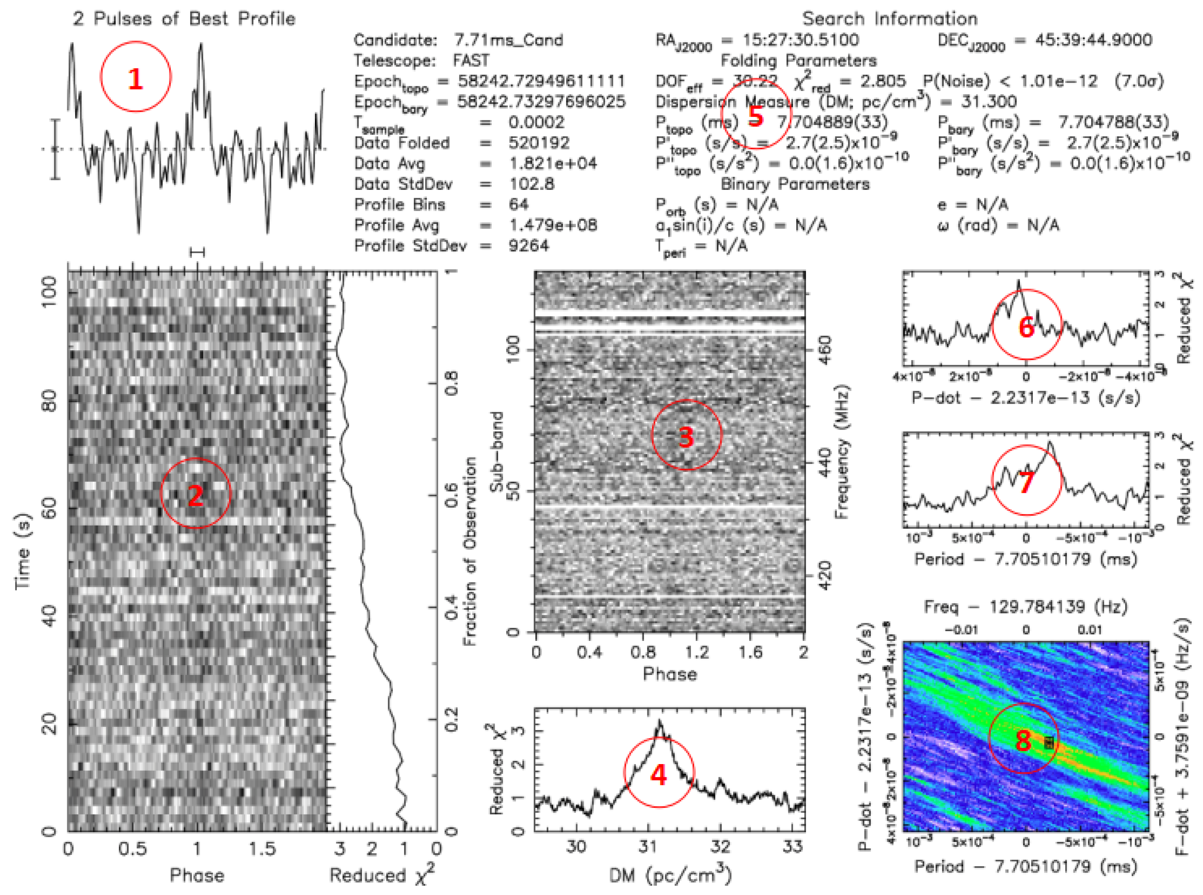Figure 1 illustrates pulsar candidate images processed by PRESTO.

Pulsar candidate diagnostic images are a fundamental basis for scientists to assess the significance of pulsars, and they also serve as a data source for machine learning methods used in pulsar selection. The labeled subfigures in Figure 1 include (1) the pulsar profile curve subfigure, (2) time–phase subfigure, (3) frequency–phase subfigure, and (4) period–dispersion subfigure. These subfigures provide essential reference features for astronomers when evaluating candidate samples. Here, our work focuses on the compression processing of subfigures (2), (3), and (4), while for the other subfigures, we will convert them into binary images using WBS (skip-white-block) encoding [24]. In the time–phase subfigure and frequency–phase subfigure of positive samples in the pulsar candidate set, we can intuitively observe a prominent stripe. This is because the phase of the pulsar signal from the same point source radiation is the same, resulting in a significant vertical correlation in the images. The center of the period–dispersion subfigure is a bright point that radiates outward in all directions. These image pixels exhibit structural correlations, which can be a key factor in image modeling.

With the activation of 19-beam observations and the utilization of parallel acceleration tools, FAST has significantly bolstered its search capabilities, resulting in the generation of a massive volume of pulsar candidate images. According to early statistics from the FAST data center, approximately 60,000 images are generated daily, accumulating to 60 GB per month and 800 GB per year. The exponential growth in the scale of astronomical scientific data stored in the form of image-based pulsar candidate images poses challenges in scientific data management.

Researching data compression techniques for compressing candidate images holds paramount importance. This research facilitates efficient data storage, accelerates network transmission and sharing, and contributes significantly to advancing astronomical scientific exploration and research.

2.2. PixelCNN

The autoregressive model decomposes the joint density distribution into a product of conditional distributions for multiple elements. Its formula is described as follows:

$$\mathrm{p}(x)={\displaystyle \prod _{i=0}^N\mathrm{p}(x_i|x_{<i})}$$

(1)

The autoregressive model demands a strict context structure, where for each element, only the preceding pixel information can be used to predict the current pixel’s density distribution. Models like MADE (masked autoregressive model estimator) [6], NADE (neural autoregressive model estimator) [7], and RANDE (real autoregressive model estimator) [7] implement this probability prediction function using neural networks. Image data contain spatial structural information, and simply flattening images into 1D sequences can lead to a significant loss of spatial information.

Hence, to address this, (Oord et al., 2016) [8] introduced the deep generative model PixelCNN. It employs convolutional neural networks to capture structural information and models the pixel probability distribution of natural images in a z-scan order. To achieve autoregressive dependencies, Oord defined two types of masked convolutional layers, as illustrated in Figure 2. The convolution kernel of a 2D convolutional layer is multiplied by a mask matrix, which constrains network connectivity relationships, ensuring compliance with autoregressive requirements. In Figure 2a, Type A convolution masks the lower-right part of the convolutional kernel information. By using Type B convolution multiple times, as shown in Figure 2b, we can expand the receptive field and extract information from the left and upper positions of the current location.

PixelCNN leverages the advantages of convolutional neural network operations. Convolutional layers are efficient at extracting spatially correlated information and can be parallelized for processing. This ensures both model training and data processing speed. However, PixelCNN also has some issues and limitations. The inherent characteristics of convolutional networks determine that PixelCNN can model local correlated information effectively, yet it struggles to efficiently utilize dependencies over longer distances. Research indicates that enlarging the receptive field is crucial for enhancing model performance. To achieve this, PixelCNN stacks multiple masked convolutional layers. However, this approach also presents the following problems:

(1)

Stacking multiple network layers increases the model’s parameters. As the network depth increases, the convergence speed of the model slows down, and it can even lead to a decrease in model performance or instability.

(2)

Despite enlarging the receptive field, the local nature of CNNs makes the model focus more on neighboring information, often neglecting crucial information from distant areas.

3. The Proposed Methods

To expand the receptive field and effectively utilize global image information, we introduce a self-attention module and residual connections to the PixelCNN framework, creating a novel network building block known as the causal residual self-attention module. This new model is referred to as the RCA-PixelCNN. In this section, we provide a comprehensive overview of the proposed model’s architecture, with a primary focus on a detailed analysis of the introduced causal residual self-attention module. We discuss the selected data distribution entropy model and present the integration of the proposed model with arithmetic coding, outlining a practical compression encoding process.

3.1. Network Architecture

As depicted in Figure 3, the proposed model primarily comprises four stages: feature extraction, residual learning, causal residual attention learning, and adjustment of output feature channels using 1 × 1 causal convolution. The blue block represents the big kernel causal convolution layer, which includes type A convolutional layers for extracting relevant features. The green block represents the small kernel causal layer, which includes type B convolutional layers to expand the receptive field. The orange block represents the residual-causal-attention block, which is our innovation and can be used to capture global feature information; detailed descriptions can be found in Section 3.2. The gray module represents the residual causal block, which can extract fine-grained features. Finally, there is a 1 × 1 causal convolution layer that can reshape the resulting features to the desired size.

3.2. Residual-Causal-Attention Block

To address the issues present in PixelCNN, we consider two approaches: residual neural networks and self-attention networks. To tackle the problem of gradient vanishing and gradient explosion caused by deep network layers, (Kaiming et al., 2016) [25] introduced residual neural networks. These networks incorporate residual learning branches into the main network using skip connections. The main network approximates the target, while the residual branch learns the difference between the main network and the target. This ensures stable performance even with increased network depth. Residual connections expand the receptive field, but convolutional networks still tend to emphasize nearby information over distant information. On the other hand, self-attention models [26] utilize a square matrix of the same length as the input data sequence to store the importance of correlations between input elements. This breaks away from the convolutional bias, allowing access to long-range information indiscriminately. However, self-attention modules access all elements of the input, rather than just the pixels preceding the current pixel in the spatial position. This limitation prevents direct utilization of self-attention modules for autoregressive modeling.

(Xi Chen, 2018) [27] analyzed the implementation process of self-attention and introduced causal attention modules by setting specific mask matrices. This allows networks containing self-attention modules to satisfy the autoregressive property. According to a certain autoregressive order, a series of 2D feature map vectors are named as $y_1,y_2,\cdots ,y_N$. The autoregressive mapping relationship is as follows:

$$z_i={\displaystyle \sum _{i<j}{p}_{ij}{f}_{value}(y_j)}$$

(2)

$$p_i=soft\max ([f_{key}{(y_1)}^T{f}_{query}(y_i),\cdots ,f_{key}{(y_{i-1})}^T{f}_{query}(y_i)])$$

(3)

The attention distribution $p_i$ corresponds to the dependency level of all features of feature ${\mathrm{y}}_{\mathrm{i}}$. Each conditional probability is established based on accessing all pixels within the attention-constrained context ${\displaystyle {\sum }_{\mathrm{j}<i}^{}{p}_{ij}=1}$. As evident from Equation (2), to achieve autoregressive conditions, it is sufficient to constrain the summation terms during the summation process.

As shown in Figure 4, this is our proposed residual-causal-attention block. The dashed box represents the causal attention module [12], which carries essential information in the main path of the network. Below it, there are three stacked masked convolutional layers, with ReLU layers and BatchNorm layers in between. The first convolutional layer has a kernel size of $1\times 1$, and the number of channels decreases by a factor as indicated by the downward-pointing arrow in Figure 4. The second convolutional layer has a kernel size of $3\times 3$ and maintains the same number of channels. The third convolutional layer has a kernel size of $1\times 1$ and restores the input’s original number of channels. During the process of information transmission within the network, the feature map dimensions remain unchanged. The attention module captures the importance of positional information, while the residual connection preserves detailed information in the features. Both the causal attention module and the residual branch impose connectivity constraints, ensuring the extracted information maintains autoregressive properties. The attention module can also employ a multi-head mechanism to enhance the weighting of importance. The residual causal attention module is an independent network module that can be used as a plugin within any part of an existing autoregressive network.

3.3. Entropy Model

Compression encoding requires the encodable information to be discrete, corresponding to a discrete density model. Most neural networks utilize continuous models for image modeling, wherein data are first quantized inversely to learn a continuous model. Encoding with such a model involves quantizing the variables first and discretizing the learned model, which is a complex process. However, we directly model discrete pixel values; each pixel is an 8-bit integer $x\in \{0, ...,255\}$, and the pixel density model becomes a 256-way categorical distribution. For example, when we input $N\times N$ image data into the model and process it through a series of network layers, we obtain the parameters of pixel density distribution with a final size of $N\times N\times 1\times 256$. The last dimension indicates the probability of the 256 possible values for each pixel. Therefore, a softmax operation is applied to the prediction features.

$$soft\max (z_i)=\frac{\exp (z_i)}{{\displaystyle \sum _{j=0}^N\exp (z_j)}}$$

(4)

Normalizing the last dimension of the model’s output ensures that the sum of the probability distribution is equal to 1, ${\displaystyle {\sum }_{\mathrm{i}=0}^{255}p(z_i)=1}$, guaranteeing that the model’s output in this dimension represents a valid probability distribution.

The model used for data compression is denoted as $q$, while the actual distribution of the data is represented by $p$. The training objective is to minimize the distance between the model $q$ and the data distribution $p$, which can be expressed as

$$\begin{array}{cc}{D}_{KL}(q(x)& \left|\right|p(x))=p(x)(\log q(x)-\log p(x))\\ & =p(x)\log q(x)-p\log p(x)\\ & =H(q,p)-H(p)\end{array}$$

(5)

So, the cross-entropy is given by

$$H(q,p)=H(p)+D_{KL}(\mathrm{q}||p)$$

(6)

where $H(p)$ represents the entropy of the data, and when the data are given, it remains constant. Therefore, minimizing the KL divergence is equivalent to minimizing the cross-entropy. Cross-entropy $H(q,p)$ represents the amount of information required to encode data using the model and is equal to the codelength. Thus, we use cross-entropy as the training objective for the compression model. In the encoding process, the autoregressive model estimates data density, and this estimation can be computed in parallel all at once. In the decoding process, on the other hand, pixel probabilities are estimated step by step during decoding. As a result, autoregressive algorithms compress data quickly, and while decompression is slower, they offer good compression performance.

3.4. Arithmetic Coding

The most commonly used entropy coding algorithm employed in this paper is the arithmetic coding. When encoding each pixel in the image, it is necessary to know the probability distribution of the pixels. The image’s pixel sequence is then transformed into a binary sequence. Based on the size of the probabilities, pixels are assigned different numbers of coding bits. The arithmetic coder assigns fewer bits to pixels with higher probabilities and more bits to pixels with lower probabilities. Another reason for choosing arithmetic coder is its progressive coding approach, which aligns well with our progressive probability model. Based on the pixels that have already been encoded, the model predicts the probabilities of pixels to be encoded next, resulting in higher compression efficiency. The decoding process follows a similar pattern. Initially, pixels that were encoded earlier are decoded, and then subsequent pixels are decoded conditionally one by one.

4. Experiments

In this section, we first introduce the dataset of pulsar candidate diagnostic images. We also present the baseline models used for comparison against the RCA-PixelCNN model, including the Gaussian mixture model (GMM), Student’s t mixture model (STM), and the PixelCNN Base Model. Subsequently, we conduct two sets of experiments. In the first set of experiments, we compare the modeling performance of the RCA-PixelCNN model against the GMM, STM, and PixelCNN Base Model. We evaluate the average negative log-likelihood values. In the second set of experiments, we analyze the proposed causal residual self-attention module through various erosion experiments, investigating different settings.

4.1. Datasets

(1)

The HTRU1 (High Time Resolution Universe Survey) dataset originates from observations conducted by the Parkes Telescope in Australia using multiple beams (13 beams). The central observing frequency is 1352 MHz, and each beam records a bandwidth of 400 MHz, with the actual data usage being in the middle 340 MHz bandwidth. This dataset comprises 1196 known pulsars (positive samples) from 512 distinct sources and 89,996 non-pulsar candidates (negative samples). Within the HTRU1 dataset’s HTRUS subset, there are 60,000 binary classification images sized 32 × 32. These images include both known pulsars and non-pulsar candidates. Each image consists of two channels, analogous to the RGB channels in natural images, although the content of each channel differs from that of natural images. Channel 1 represents the period–dispersion subgraph, channel 2 corresponds to the frequency–phase subgraph, and channel 3 represents the time–phase subgraph. The left four columns in Figure 7 depict the positive samples from the HTRU1 dataset, where the first row shows the period–dispersion graph, the second row displays the frequency–phase graph, and the third row depicts the time–phase graph. In this study, the HTRU1 dataset is utilized for training, testing, and validating the models. The baseline models, including the GMM and STM, require the data to be in the form of 1D tensors. Therefore, the 2D images need to be reshaped into 1D sequences before being used with these models. On the other hand, both the PixelCNN baseline model and the RCA-PixelCNN model are capable of directly processing structured image data without the need for reshaping.

(2)

FAST Pulse Candidate Data: The FAST pulse candidate images are obtained from 19-beam observations using the PRESTO software processing. These image-formatted pulse candidate data files are sourced from the early data center of FAST and are intended for internal use. In practical applications, the model is initially trained using the HTRU1 dataset. Subsequently, transfer learning is applied to fine-tune the model parameters on the FAST data, ensuring the model’s better suitability for the specific application scenarios of FAST.

4.2. Baseline Models

(1)

GMM: The Gaussian mixture model consists of multiple Gaussian distributions as its components. Each image is associated with a Gaussian distribution, making it suitable for data spaces with multiple central distributions. As long as the model has a sufficient number of components, it can approximate any complex distribution.

(2)

STM: The Student’s t mixture model, similar to the GMM, employs Student’s t-distribution as its components. It is particularly well suited for modeling data distributions with heavy tails, as seen in natural images.

(3)

PixelCNN Base Model: This is a typical autoregressive model that works well for data with spatial structure. By stacking multiple masked convolutional layers, the receptive field can be expanded. In this context, the baseline model includes one type A masked convolutional layer with a kernel size of 7 × 7, two type B masked convolutional layers with kernel sizes of 3 × 3, and one type B masked convolutional layer with a kernel size of 1 × 1.

4.3. Evaluation Metric

In theory, the negative log likelihood corresponds to the codelength in lossless compression, so a smaller negative log-likelihood score for the compression model indicates a higher compression ratio. The calculation of the negative log-likelihood score is as follows:

$$NLL(\theta )=E_{x~p(x)}-\log q_{\theta }(x)$$

(7)

where $p(x)$ is the image data distribution, $q_{\theta }(x)$ is the model distribution, and $\theta$ is the model parameters, which manifest as neural network weights. For image data, the unit of log-likelihood value can be denoted as “bpp” (bits per pixel).

4.4. Results and Analysis

4.4.1. Experiment Setting and Results

The model in this paper was implemented using the PyTorch framework on an NVIDIA GeForce GTX 1080 GPU. The implementation details of the model structure are as follows: At the front end of the network, a large-sized convolutional layer with a 7 × 7 kernel of type A is used, with 3 input channels and 128 output channels, followed by a BatchNorm layer and a ReLU activation function layer. Immediately following is a small-sized 3 × 3 convolutional layer with a kernel of type B, also having 128 input and output channels, and including a BatchNorm layer and a ReLU activation function layer. There are seven Residual Causal layers, where the residual branch structure is Conv B_1 × 1 → BatchNorm → ReLU → Conv B_3 × 3 → BatchNorm → ReLU → Conv B_1 × 1. The first convolutional layer has 128 input channels and 64 output channels, the second convolutional layer has 64 input and output channels, and the last convolutional layer has 64 input channels and 128 output channels. The main path is connected to the residual branch by adding their information. The residual-causal-attention block was injected as a plugin into the main network, and its implementation details were introduced in Section 3.2. Finally, there is a 1 × 1 Causal Convolution layer with a 1 × 1 kernel of type B, having 128 input channels and 256 output channels. As can be seen, we do not stack Conv B layers to expand the receptive field; instead, we use Residual Causal Attention and Residual Casual Layers. The optimizer used is Adam, with an initial learning rate of 0.01 and beta parameters of 0.9 and 0.99.

In order to make a fair comparison of the density modeling abilities between RCA- PixelCNN and the GMM (Gaussian mixture model) as well as STM (Student’s t mixture model), the evaluation metric used is the average negative log likelihood. Both training and testing data are sourced from the HTRU1 dataset. Our RCA-PixelCNN model directly models 2D image matrices and 3D data volumes, whereas the GMM and STM can only model 1D data sequences. Since the HTRU1 images are of size 64 × 64, they are flattened to 1D, resulting in a dimensionality of 4096. Due to the high dimensionality, convergence of models like the GMM and STM becomes challenging. To address this issue, for the training set, we randomly extract 800,000 8 × 8 image patches from the training data. Through model selection experiments, we determine the optimal number of mixture components for the GMM and STM to be 8. To avoid overfitting or underfitting, the models are trained on the training set, and their performance in terms of average negative log likelihood is evaluated using the test set.

As shown in

Table 1. Comparison of RCA-PixelCNN with other models in terms of negative log likelihood (NLL).

Methods	NLL (bpp)
GMM	3.54
STM	4.11
PixelCNN Base Model	3.11
RCA-PixelCNN	2.82

, we compare the experimental results of RCA-PixelCNN with other models on the HTRU1 test dataset. The average negative log-likelihood score for the mixtures of the Gaussian model is 3.51 bits per pixel (bpp), which performs well in fitting natural images. However, the mixtures of the Student T model, which is typically better suited for long-tailed distributions, perform worse than the GMM, suggesting that the candidate pulse images do not follow a long-tailed distribution. The PixelCNN model achieves an average negative log-likelihood score of 3.11 bpp, indicating the best performance among the compared models. This highlights the superior modeling capability of neural-network-based methods compared to traditional approaches. Within the PixelCNN framework, the RCA-PixelCNN model with the added Res-Causal-Attention module exhibits the best performance, outperforming the standard PixelCNN by 0.33 bpp. This demonstrates that deep-learning-based modeling methods outperform traditional data distribution modeling approaches, and the inclusion of the Res-Causal-Attention module further enhances the performance of PixelCNN.

In Figure 5, we present the training curves for the PixelCNN Base Model and the RCA-PixelCNN. It is evident that the training speed of our model is slower compared to the baseline PixelCNN model. The training time per batch is approximately 10 times that of the baseline model. Additionally, our model requires higher memory resources, and due to memory limitations, the batch size for training is smaller than that of the baseline model. This can lead to greater fluctuations in the convergence during training. After adjusting the learning rate and performing subsequent training epochs, the convergence gradually stabilizes. The experimental results demonstrate that the stability and performance of our RCA-PixelCNN model significantly outperform the baseline PixelCNN model.

4.4.2. Practical Coding Algorithm

In the actual data compression process, we combine the proposed RCA-PixelCNN model with arithmetic coding to achieve efficient data compression. The specific process is as follows:

Model Training: Firstly, we train the RCA-PixelCNN model using the HTRU1 dataset to obtain a model that accurately models the data distribution.

Density estimation: Using the trained RCA-PixelCNN model, we input the data to be compressed into the model. The model predicts the probability distribution of each pixel based on its density distribution model.

Encoding: We use the arithmetic coding algorithm for actual compression encoding. This algorithm maps the pixel sequence to a compact binary encoding based on the predicted probability distribution from the model. High-probability pixels are assigned fewer bits, while low-probability pixels are assigned more bits.

Decoding: We predict the probability distribution of each pixel using the trained model and previous decoded pixels. Then, we use the arithmetic coding algorithm to reverse the encoding process, recovering the original pixel sequence from the binary encoding.

We provide detailed pseudocode descriptions of the arithmetic encoding and decoding processes based on the RCA-PixelCNN in Algorithm 1.

Algorithm 1: Arithmetic coding with RCA-PixelCNN. [AC] stands for arithmetic coding

Encoder:     use our model to compute: $a_i=p(x_i|x_1,\cdots ,x_{i-1})$,$i\in \{1,2,\cdots ,D\}$ for each $x_i$, $i=1,2,\cdots ,D$ do [AC] enode symbol $x_i$ with probability $a_i$     end for Decoder: for each $x_i$, $i=1,2,\cdots ,D$ do with decoded pixels $x_1,\cdots ,x_{i-1}$, use our model to compute: $a_i=p(x_i|x_1,\cdots ,x_{i-1})$ [AC] decode symbol $x_i$ with probability $a_i$     end for

4.4.3. Ablation Experiments

In order to test the impact of specific module modifications on the overall model, we conducted a series of erosion experiments and analyses. Firstly, we compared the performance difference between the causally connected attention module without residual connections and the existing combination method. Secondly, we examined the effect of stacking different numbers of Res-Causal-Attention modules in the network on the overall model. Through these experiments, our aim was to gain a deeper understanding of how these specific module modifications affect the model’s performance.

(1)

Skip connection

To validate the impact of residual connections on the model, without the loss of generality, we retained the Causal-Attention part of a module and removed the Resnet Connection within the module. All connection layers were placed in the main network, maintaining the same depth and parameter count as the existing model. The comparison of training curves between the model with severed residual connections and the existing model is shown in Figure 6a. Our model achieved a negative log-likelihood score of 2.82 bpp, while the model without residual connections achieved a score of 2.99 bpp. The performance difference is 0.17 bpp. This indicates that residual connections have a significant impact on model performance. The sub-images of pulsar candidates contain a substantial amount of random noise, and the pulsar signal features exhibit subtle differences from noise, highlighting the importance of preserving details through learning.

(2)

Causal Attention

In Section 3.2, it was mentioned that the attention module can break the limit of the receptive field size in convolutional networks. It extracts information from different positions with varying degrees of attention and computes a weighted sum of contextual information as the predicted probability distribution for the current pixel. To evaluate the role of the self-attention module in the entire network model and understand its effect on improving model performance, we conducted experiments by removing the attention module and comparing it with the existing model.

The results are shown in Figure 6b. The model without the attention module achieved a log-likelihood value that is 0.4 bits per pixel lower than our model. The convergence speed of the network is slower, but the memory consumption is slightly reduced. This is because the test dataset, HTRU1 images, has a size of 32 × 32 pixels, which is of medium size. The effect of the attention module is more pronounced on larger images, and overall performance improvement is moderate. However, in practical scenarios, the images of FAST pulsar candidates that need to be compressed are larger, indicating that the impact of the attention module could be more substantial in those cases.

(3)

Numbers of Res-Causal-Attention

The Res-Causal-Attention module was added as a plugin module to the neural network, and different numbers of Res-Causal-Attention modules were set. The comparison of negative log-likelihood scores is shown in

Table 2. Comparison of model with different numbers of Res-Cause-Attention blocks.

Methods	NLL (bpp)
PixelCNN	3.11
RCA-PixelCNN-1	2.82
RCA-PixelCNN-2	2.78

. In the PixelCNN network, adding one Res-Causal-Attention module improved the performance by 0.29 bpp, and adding two Res-Causal-Attention modules improved the performance by 0.33 bpp. Due to the memory-intensive nature of the attention mechanism in the Res-Causal-Attention module, and considering the limitations of the experimental environment, we stacked up to two Res-Causal-Attention blocks.

The experiments demonstrate that the Res-Causal-Attention module significantly improves model performance, and as the number of modules increases, the model performance continues to improve. In the experiments, we attempted to replace self-attention with multi-head self-attention and found that the multi-head mechanism also effectively enhances the model. The multi-head mechanism essentially increases the number of attention channels, achieving a similar effect as deep stacking. The significant impact of the Attention module can also be explained by the characteristics of the pulsar sub-images. For instance, the sub-integration phase image, which is a folded representation of pulsar data, exhibits clear overlapping and similarity regions in positive samples. The expanded receptive field of the convolution operation makes effective use of the vertical pixel correlations in this scenario.

4.5. Generated Positive Pulsar Candidate Samples

Pulsar observation data suffer from severe class imbalance in classification tasks. As of now, there are over 3000 confirmed pulsars, while the number of daily pulsar candidate observations reaches hundreds of thousands. Candidate selection is a crucial aspect of pulsar search efforts. Taking the HTRU1 dataset as an example, the positive–negative sample ratio is 1194:58,806, with positive samples accounting for only 2% of the total. Machine learning is employed to sift through pulsar candidates, and addressing class imbalance is a primary concern [28].

Using a class-label conditioned PixelCNN model can generate the required positive samples. We encode the class information using one-hot encoding and linearly map it to features of the same shape as the images. The label features are input to each layer. The three sub-images of each synthetic HTRU1 sample describe the same candidate’s information, and the three-channel sub-images are interdependent. As shown in the rightmost four columns of Figure 7, the positive samples generated by the class-conditioned PixelCNN model are displayed. The three rows of sub-image correspond to period–dispersion, time–phase, and frequency–phase representations. It is evident that the generated positive samples exhibit distinct pulsar characteristics.

5. Conclusions and Discussion

We analyzed the distinctive features of various subfigures in the pulsar candidate diagnostic images and identified the limitations of the baseline models. In the time–phase subfigure and frequency–phase subfigure of positive samples in the pulsar candidate set, we can intuitively observe a prominent stripe. The center of the period–dispersion subfigure is a bright point that radiates outward in all directions. These image pixels exhibit structural correlations, which can be a key factor in image modeling. However, the GMM and STM can only model 1D sequences, and flattening the image disrupts its structural information. PixelCNN uses convolutional layers to extract features, effectively preserving spatial structural characteristics. However, the local nature of convolutional layers makes the PixelCNN model more likely to focus on nearby information and ignore important information at greater distances. To expand the receptive field, PixelCNN must stack multiple convolutional layers. Unfortunately, deepening the network can affect information propagation and lead to issues such as gradient vanishing.

We proposed an RCA-PixelCNN model for pulsar candidate image compression. The core module proposed in this model, the residual-causal-attention block, defines a masked weight matrix to assess the importance of each pixel’s position in the image. This block not only breaks the local constraints of convolution operations but also preserves positional dependencies in autoregressive networks. Additionally, the residual connection captures crucial image details, preventing feature information from being overwhelmed by noise. RCA-PxieCNN utilizes multiple Residual Causal Attention layers and Residual Casual Layers to expand the information receptive field, effectively capturing the global structural information of the image. We conducted experiments using the HTRU1 dataset to evaluate the RCA-PixelCNN model, calculating its average negative log-likelihood score. The results demonstrate that the negative log-likelihood score of RCA-PixelCNN surpasses that of existing prominent density models such as the GMM, STM, and PixelCNN.

Furthermore, we addressed the issue of class imbalance. For pulsar candidate images, we employed a class-conditioned PixelCNN model to generate positive samples. By learning class information, we successfully generated images with distinct pulsar features. This work may be meaningful for machine learning methods in pulsar candidate sifting.

References

- Li, D.; Wang, P.; Qian, L.; Krco, M.; Dunning, A.; Jiang, P.; Yue, Y.L.; Jin, C.J.; Zhu, Y.; Pan, Z.C.; et al. FAST in Space: Considerations for a Multibeam, Multipurpose Survey Using China’s 500-m Aperture Spherical Radio Telescope (FAST). IEEE Microw. Mag. 2018, 3, 112–119. [Google Scholar] [CrossRef]
- Pence, W. CFITSIO, v2.0: A new full-featured data interface. Astron. Data Anal. Softw. Syst. VIII 1999, 172, 487. [Google Scholar]
- Cosemans, A.; Batelaan, O.; Louwyck, A.; Lermytte, J. Hierarchical data format (HDF5) for Modflow, Modpath and ZoneBudget. In Proceedings of the EGU General Assembly, Vienna, Austria, 22–27 April 2012; EGU General Assembly: Munich, Germany, 2012. [Google Scholar]
- Zoran, D.; Weiss, Y. Natural images, Gaussian mixtures and dead leaves. In Proceedings of the 25th Conference on Neural Information Processing Systems, Lake Tahoe, NV, USA, 3–6 December 2012. [Google Scholar]
- Oord, A.V.D.; Schrauwen, B. The student-t mixture as a natural image patch prior with application to image compression. J. Mach. Learn. Res. 2014, 15, 2061–2086. [Google Scholar]
- Gregor, M.; Murray, K.; Murray, I.; Larochelle, H. Made: Masked autoencoder for distribution estimation. In Proceedings of the 32nd International Conference on Machine Learning, Lille, France, 6–11 July 2015. [Google Scholar]
- Uria, B.; Côté, M.A.; Gregor, K.; Murray, I.; Larochelle, H. Neural autoregressive distribution estimation. J. Mach. Learn. Res. 2016, 17, 7184–7220. [Google Scholar]
- Oord, A.V.D.; Kalchbrenner, N.; Kavukcuoglu, K. Pixel recurrent neural networks. In Proceedings of the 33rd International Conference on Machine Learning, New York, NY, USA, 19–24 June 2016. [Google Scholar]
- Oord, A.V.D.; Kalchbrenner, N.; Espeholt, L.; Vinyals, O.; Graves, A. Conditional image generation with pixelcnn decoders. In Proceedings of the 30th International Conference on Neural Information Processing Systems, Banrcelona, Spain, 5–10 December 2016. [Google Scholar]
- Sønderby, C.K.; Raiko, T.; Maaløe, L.; Sønderby, S.K.; Winther, O. Ladder variational autoencoders. In Proceedings of the 30th International Conference on Neural Information Processing Systems, Banrcelona, Spain, 10 December 2016. [Google Scholar]
- Zhang, Z.Y.; Sun, L.; Zheng, Z.; Li, Q. Disentangling the spatial structure and style in conditional vae. In Proceedings of the 2020 IEEE International Conference on Image Processing (ICIP), Abu Dhabi, United Arab Emirates, 25–28 October 2020. [Google Scholar]
- Levy, S.; Laloy, E.; Linde, N. Variational Bayesian inference with complex geostatistical priors using inverse autoregressive flows. Comput. Geosci. 2023, 171, 105263. [Google Scholar] [CrossRef]
- Papamakarios, G.; Nalisnick, E.; Rezende, D.J.; Mohamed, S.; Lakshminarayanan, B. Normalizing flows for probabilistic modeling and inference. J. Mach. Learn. Res. 2021, 22, 2617–2680. [Google Scholar]
- Kingma, D.; Salimans, T.; Poole, B.; Ho, J. Variational diffusion models. In Proceedings of the 35th Conference on Neural Information Processing Systems (NIPS), Virtual, 6–14 December 2021; Volume 34, pp. 21696–21707. [Google Scholar]
- Huang, C.W.; Lim, J.H.; Courville, A.C. A variational perspective on diffusion-based generative models and score matching. In Proceedings of the 35th Conference on Neural Information Processing Systems (NIPS), Virtual, 6–14 December 2021; Volume 34, pp. 22863–22876. [Google Scholar]
- Witten, I.H.; Neal, R.M.; Cleary, J.G. Arithmetic Coding for data compression. Commun. ACM 1987, 30, 520–540. [Google Scholar] [CrossRef]
- Townsend, J.; Bird, T.; Barber, D. Practical lossless compression with latent variables using bits back coding. In Proceedings of the 35th International Conference on Learning Representations (ICML), Long Beach, CA, USA, 9–15 June 2019. [Google Scholar]
- Kingma, F.; Abbeel, P.; Ho, J. Bit-swap: Recursive bits-back coding for lossless compression with hierarchical latent variables. In Proceedings of the 36th International Conference on Machine Learning (ICML), Long Beach, CA, USA, 9–15 June 2019; pp. 3408–3417. [Google Scholar]
- Townsend, J.; Bird, T.; Kunze, J.; Barber, D. Hilloc: Lossless image compression with hierarchical latent variable models. In Proceedings of the International Conference on Learning Representations (ICLR), Addis Ababa, Ethiopia, 26–30 April 2020. [Google Scholar]
- Ho, J.; Lohn, E.; Abbeel, P. Compression with flows via local bits-back coding. In Proceedings of the 33rd International Conference on Neural Information Processing Systems (NIPS19), Vancouver, Canada, 8–14 December 2019; pp. 3879–3888. [Google Scholar]
- Qian, L.; Pan, Z.C.; Li, D.; Hobbs, G.; Zhu, W.W.; Wang, P.; Liu, Z.J.; Yue, Y.L.; Zhu, Y.; Liu, H.F.; et al. The first pulsar discovered by FAST. Sci. China Phys. Mech. Astron. 2019, 62, 1–4. [Google Scholar] [CrossRef]
- Pan, Z.; Ransom, S.M.; Lorimer, D.R.; Fiore, W.C.; Qian, L.; Wang, L.; Stappers, B.W.; Hobbs, G.; Zhu, W.; Yue, Y. The FAST Discovery of an Eclipsing Binary Millisecond Pulsar in the Globular Cluster M92 (NGC 6341). Astrophys. J. Lett. 2020, 892, 5. [Google Scholar] [CrossRef]
- Wang, Y.C.; Li, M.T.; Pan, Z.C.; Zheng, J.H. Pulsar candidate classification with deep convolutional neural networks. Res. Astron. Astrophys. 2019, 19, 133. [Google Scholar] [CrossRef]
- Jiang, J.T.; Xie, X.Y.; Yu, X.H. Research on Compression of Pulsar Candidate Diagnostic Image Based on WBS and Deep Neural Network. Astron. Res. Technol. 2022, 19, 470–478. [Google Scholar]
- He, K.; Zhang, X.; Ren, S.; Sun, J. Deep residual learning for image recognition. In Proceedings of the IEEE Conference on Computer Vision and Pattern Recognition (CVPR), Las Vegas, NV, USA, 26 June–1 July 2016; pp. 770–778. [Google Scholar]
- Vaswani, A.; Shazeer, N.; Parmar, N.; Uszkoreit, J.; Jones, L.; Gomez, A.N.; Polosukhin, I. Attention is all you need. In Proceedings of the 31st International Conference on Neural Information processing systems (NIPS17), Long Beach, CA, USA, 4–9 December 2017; pp. 6000–6010. [Google Scholar]
- Chen, X.; Mishra, N.; Rohaninejad, M.; Abbeel, P. Pixelsnail: An improved autoregressive generative model. In Proceedings of the 35th International Conference on Machine Learning (PMLR), Stockholm, Sweden, 10–15 July 2018; Volume 80, pp. 864–872. [Google Scholar]
- Morello, V.; Barr, E.D.; Bailes, M.; Flynn, C.M.; Keane, E.F.; Straten, W.V. SPINN: A straightforward machine learning solution to the pulsar candidate selection problem. Mon. Not. R. Astron. Soc. 2014, 443, 1651–1662. [Google Scholar] [CrossRef]