Gait Recognition Based on Gait Optical Flow Network with Inherent Feature Pyramid

Abstract

Gait is a kind of biological behavioral characteristic which can be recognized from a distance and has gained an increased interest nowadays. Many existing silhouette-based methods ignore the instantaneous motion of gait, which is an important factor in distinguishing people with similar shapes. To further emphasize the instantaneous motion factor in human gait, the Gait Optical Flow Image (GOFI) is proposed to add the instantaneous motion direction and intensity to original gait silhouettes. The GOFI also helps to leverage both the temporal and spatial condition noises. Then, the gait features are extracted by the Gait Optical Flow Network (GOFN), which contains a Set Transition (ST) architecture to aggregate the image-level features to the set-level features and an Inherent Feature Pyramid (IFP) to exploit the multi-scaled partial features. The combined loss function is used to evaluate the similarity between different gaits. Experiments are conducted on two widely used gait datasets, the CASIA-B and the CASIA-C. The experiments show that the GOFN performs better on both datasets, which shows the effectiveness of the GOFN.

1. Introduction

Gait recognition has attracted much attention because it can identify an individual from a distance without subject cooperation. Compared with other biometrics such as face, fingerprint, and iris recognition, gait recognition identifies a person from their walking style, which is hard to disguise. However, gait recognition suffers from many variations, such as clothing, carrying conditions, and camera viewpoint [1]. A key challenge for gait recognition is effectively leveraging the condition noises and extracting the invariant gait features.

Many approaches have been proposed to extract gait features. A gait energy image (GEI) [2] aggregates the silhouette sequence into one image to represent gait. However, it is sensitive to some variations, such as camera viewpoint and carrying conditions. Moreover, more representation methods are proposed based on GEIs to improve the accuracy, such as the gait history image (GHI) [3], the frame difference energy image (FDEI) [4], and the active energy image (AEI) [5]. They can represent not only the moving part but also the non-moving part of the subject, but they all transform the silhouette sequence into one image or gait template and cannot effectively represent the temporal feature. Differently, some methods treat the gait sequence as a video. For example, 3D-CNN is used to obtain the spatial and temporal features in [6,7], but it requires more effort to train and works inefficiently. Inspired by [8], some approaches based on unordered sets have been recently proposed. For example, ref. [9] regards the gait sequence as an unordered set and makes progress, although the method remains to be improved.

However, most of the above works focus on the silhouettes and rely on a data- driven network to learn long-term motion features from the silhouette sequences. These methods ignore the short-term motion features, i.e., the instantaneous motion features. To overcome this issue, the Gait Optical Flow Image (GOFI) is presented in this paper to add the instantaneous motion direction and intensity to original gait silhouettes. The GOFI also helps to leverage both the temporal and spatial condition noises. Spatial condition noises, such as clothes, will change the shape of the body, but the instantaneous motion of clothes will be the same as the body. The temporal condition noises such as the walking speed will change the cycle and phase of the gait but will maintain the same instantaneous motion direction. The GOFIs are obtained by cropping the original silhouette sequence and combining the optical flow images with the outline of the corresponding silhouettes in a particular proportion. The GOFIs can avoid the influence of silhouette distortion, which happens frequently in gait sequences. Then, a Gait Optical Flow Network (GOFN) is proposed, which contains the Set Transition (ST) architecture to fuse the image-level and the set-level features and the Inherent Feature Pyramid (IFP) to exploit the multi-scaled partial features from the GOFIs.

In summary, the main contributions of this work include the following: (1) The GOFI representation is proposed to describe the instantaneous motion direction and intensity feature, which is robust to the temporal and spatial condition noises. (2) A GOFN is proposed, which contains the Set Transition (ST) architecture to aggregate the image-level features to the set-level features and the Inherent Feature Pyramid (IFP) to exploit the multi-scaled partial features from the GOFIs. (3) The experiments and comparisons on the CASIA-B and the CASIA-C gait datasets show that the GOFN achieves better performances than previous methods under both the cross-view condition and the identical-view condition, which proves the effectiveness of the GOFN.

The rest of the paper is organized as follows: Section 2 elaborates on the related works and the ideas that inspire our work. Section 3 introduces the GOFI and the ST component and IFP component of the GOFN. Section 4 presents the dataset, the settings details, and the experimental analyses. Section 5 draws the conclusions.

2. Related Work

2.1. Gait Representation

Most prior works can be divided into appearance-based methods and model-based methods. Appearance-based approaches include GEI [2], GHI [3], gait entropy image (GEnI) [10,11,12,13], and so on. These approaches directly extract the feature from the silhouette sequences without modeling the skeleton structure. For example, GEI represents the whole gait sequence with the averaged silhouette image. This type of method can be severely influenced by variations such as clothing, bagging, and camera view. Some appearance-based approaches also take the image sequence as input, which concerns more temporal information, such as the GaitSet [9], GaitPart [14], GaitGL [15], GaitNet [16], and GaitBase approaches [17]. On the other hand, model-based approaches [18,19,20] extract the skeleton or body structure and then obtain features from a graph model, such as GaitGraph [21]. However, these approaches are usually inefficient and only work when the resolution of the gait videos is high. By comparing the neighbor joint, the short-term motion of the joint is described. Inspired by joint motion, the short-term motion of the silhouette is considered in this paper to describe more temporal features.

2.2. Unordered Set

The conception of the unordered set is proposed in [8]. The unordered set is used in point cloud research, and it was introduced into gait recognition in [9,22,23]. The experiments in these methods show that gait sequences can be regarded as unordered sets, which obtain a higher gait recognition accuracy, especially in cross-view cases. To avoid the influence of multiple views and obtain the set-level features, the unordered set of GOFI is applied by using the permutation invariant function. Moreover, the experiments prove that this method is effective and robust. Moreover, the design of the permutation invariant function is better than traditional functions.

2.3. Instantaneous Motion Description

Optical flow is a method that uses the change in the pixels of an image sequence in the temporal domain and the correlation between adjacent frames to find the correspondence between the previous and current frames to calculate the object’s motion information between adjacent frames. The authors of [24,25] introduced two kinds of methods to calculate optical flow. Since then, optical flow has been commonly used in action recognition and action detection, such as in [26,27]. Moreover, optical flow has yet to be used widely in gait recognition. It was applied in gait recognition in [28]. Nevertheless, the method simply sends the optical flow extracted from the gait sequences into a convolutional neural network, and the experiments remain to be improved.

3. Proposed Approach

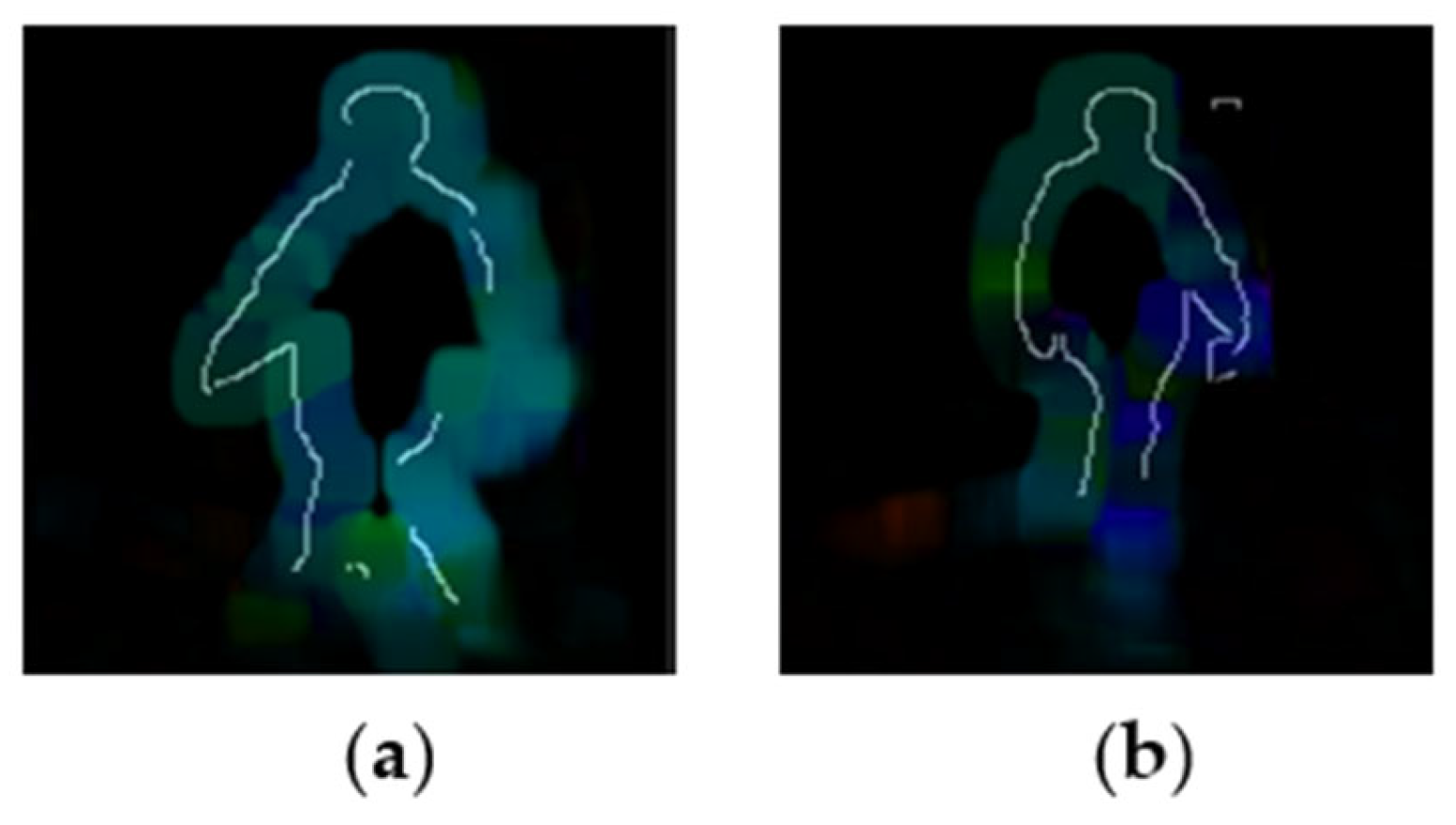
3.1. Gait Optical Flow Image Extraction

To distinguish people based on their gait sequences, the GOFI representation describes the instantaneous motion using the optical flow descriptor. The GOFI retains both temporal and spatial condition features while preserving the invariant gait features.

For a three-channel RGB gait image model, first the image is subtracted from the background image and transformed into a binary image. Then, the outlier points and the holes caused by the subtraction are eliminated using morphological operations. The center of the subject is detected using the intensity distribution. For some samples, the person is too close to the camera, and the image is filled with foreground, so these samples, in which the sum of pixel intensities is large, are eliminated. Then, the method introduced by [26] is used to calculate the two-channel optical flow matrix [u, v]. The optical flow of each pixel draws the direction and the intensity of body movement at the next step. Assuming the brightness is constant and the movement is tiny, the optical flow matrix is calculated as follows:

$$I_{x}u+I_{y}v+I_t=0$$

(1)

where I_x and I_y are, respectively, image gradients in the vertical and horizontal direction, which can be obtained using the Sobel filter, and I_t represents the temporal gradient, which can be obtained using the frame differential method. Then, the optical flow is transformed into an HSV image formulated as

$$H_{i,j}={\tan }^{-1}\frac{u_{i,j}}{v_{i,j}}$$

(2)

where, for a location (i, j), $H_{i,j}$ is the hue of the pixel and $u_{i,j}$ and $v_{i,j}$ are the optical flow component in the vertical and horizontal directions of the pixel, respectively.

$$S_{i,j}=\sqrt{{u_{i,j}}^2+{v_{i,j}}^2}$$

(3)

where $S=\left\{S_{i,j}\right\}$ means the magnitude map and $S_{i,j}$ is the magnitude at the pixel.

$$V_{i,j}=\frac{S_{i,j}}{\mathit{max}\left(S\right)-\mathit{min}\left(S\right)}$$

(4)

where $V_{i,j}$ means the value of the pixel.

As shown in Figure 1, the HSV image $I_1$ is merged with the silhouette edge image $I_2$. To obtain $I_2$, the origin image is transformed into a grayscale image and then the Canny operator is applied to detect the border of the character image. Only the edge is used instead of the whole silhouette because we are more concerned about the instantaneous motion, which is more obvious at the edges but is confusing inside the silhouette. The gait optical flow image model $I_3$ is formulated as

$$I_3=\sigma I_1+\left(1-\sigma \right)I_2$$

(5)

where $\sigma$ represents the intensity factor. Finally, the original silhouette is cropped into subject-centered images whose size is 64 × 64 to obtain the GOFI.

3.2. Set-Level Feature from Unordered Set

Assume a gait dataset contains N objects, and the corresponding gait sequence is $X=\left\{X_i\right\}$, where i ∈ 1, 2, 3, …, N. The process to transform the origin gait sequences into the GOFI representation can be formulated as follows:

$$G_i=P\left(X_i\right)$$

(6)

where P represents the process of fusing the optical flow and the silhouette edge, and $G=\left\{G_i\right\}$, where i ∈ 1, 2, 3, …, N represents the GOFI output. Then, the gait model, named GOFN, is used to extract both the image-level $f_{IL}$ and set-level feature $f_{SL}$ for higher recognition accuracy. The set-level feature can be formulated as follows:

$$f_{SL}=ST\left(f_{IL}\right), where f_{IL}=L\left(G\right)$$

(7)

where $L$ represents a group of CNN layers used to extract image-level features $f_{IL}\in {\mathbb{R}}^{d_n\times {d_c\times d}_l}$, $d_n$ is the batch size, $d_c$ is the number of channels, and $d_l$ is the length of the image-level feature. The Set Transition (ST) blocks are used to aggregate the image-level features to the set-level features.

To aggregate the temporal information and obtain set-level features from unordered gait sequences, a permutation invariant function is need to process the image-level features extracted by the CNN. Regardless of the order of objects in the set, the value of a permutation invariant function remains the same. As shown in Figure 2, the ST block can be represented as follows, where ꞷ denotes the parameters in ST block:

$$ST\left(f\right)=LN\left(f+rFL\left(f\right)\right),$$

(8)

where $f=LN\left(f_{IL}+Multihead\left(f_{IL},f_{IL},f_{IL};\mathrm{ꞷ}\right)\right)$.

LN is the layer normalization, FL is the row-wise feedforward layer, and r is the weight factor. $Multihead$() is the multi-head attention, which collects the global information to refine image-level features. First, $f_{IL}$ is copied and input into multiple linear layers to extract the multi-head subspace features. The length of subspace features is $d_{sub}$. For example, in head 0, the multi-head subspace features are denoted as ($f_q^0, f_k^0, f_v^0$). The attention $z^0$ is calculated by $z^0=softmax(f_q^0{f}_k^{0T}/\sqrt{d_{sub}})\times f_v^0$. The attentions of each head are then concatenated. The output is resized to the original shape by multiplying it with a linear layer. The output is then fed into the FL module. Each feature is multiplied with a share-weight linear layer, and the outputs are aggregated. ST takes the unordered gait sequences and applies self-attention between the image-level features, resulting in set-level features of the same size. The image-level feature is transformed to the set-level feature through ST. The structure will stabilize the network and is beneficial for recognition accuracy.

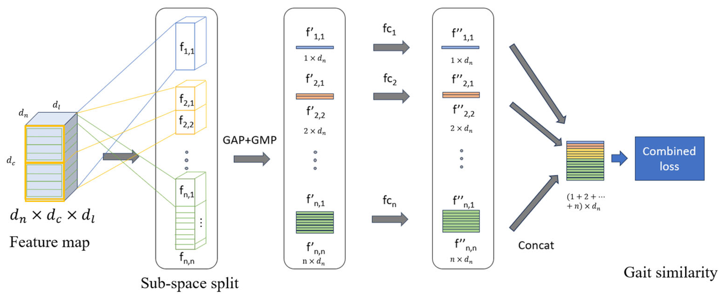
3.3. Inherent Feature Pyramid

Handled by a group of CNN layers and the ST blocks, both the temporal and the spatial information of the GOFI are extracted and transformed into a feature map with size $d_n\times {d_c\times d}_l$. $d_n$ is the batch size, $d_c$ is the number of channel, and $d_l$ is the length of the features. To capture the discrimination of the feature map from the global to local levels, from coarse to fine at various scales, the feature map is sliced into multiple-scale sub-spaces horizontally. The sub-spaces are pooled via global average pooling (GAP) and global max pooling (GMP) to obtain the feature vectors. GAP calculates the average of all pixels, and GMP calculates the maximum of all pixels for each feature map. As shown in Figure 3, the feature map is equally divided into several spatial bins as $f_{i,j}$ in a horizontal manner according to different scales. $i\in \{\mathrm{1,2},\dots ,n\}$ indicates the index of sub-space, and $j\in \{\mathrm{1,2},\dots ,n\}$ stands for the index of the bin in the sub-space. Then, each bin $f_{i,j}$ is pooled and obtains feature vector $f_{i,j}^{\prime }$, formulated as follows:

$$f_{i,j}^{\prime }=GAP\left(f_{i,j}\right)+GMP\left(f_{i,j}\right)$$

(9)

The fully connected (fc) layers are then applied for every feature vector $f_{i,j}^{\prime }$ to learn the discrimination, and the outputs $f_{i,j}^{″}$ are concatenated. To limit the length of the concatenated feature, the feature map is divided into {1, 2, 4, 8, $16, 32, 64$} sub-spaces. So, the size of the concatenated gait feature is $d_n\times$ 127. The IFP is used for mapping the feature to the discriminative spaces, while taking account of both global and local details. Both the local and global information is emphasized. Finally, the combined loss function is used to evaluate the similarity of IFP gait features, which contains the triplet loss and the cross-entropy loss to train the network.

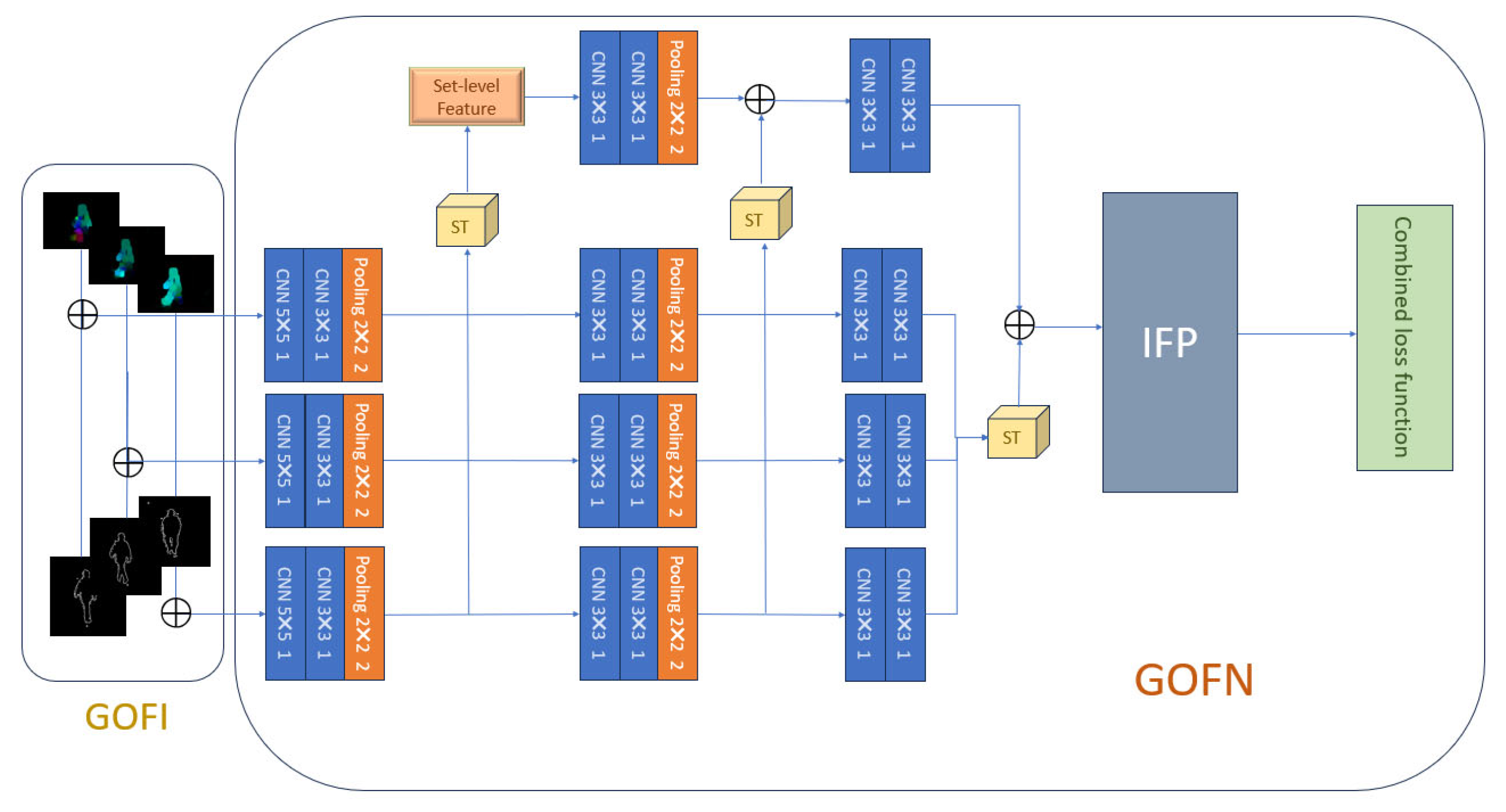
3.4. Framework of GOFN

The framework of the GOFN is shown in Figure 4. The GOFI combines the optical flow and the silhouette edge, which describes both the instantaneous motion and the shape. Then, each GOFI is input to a CNN block to obtain the image-level feature, which contains a $5\times 5$ layer, a $3\times 3$ layer, and a $2\times 2$ pooling layer. Then, the ST block aggregates the image-level features into the set-level features. The set-level features are spitted and concatenated in the IFP block to balance the global and local features. The output features of the IFP are used to compute the similarity between different gaits. The gait features with annotated IDs are used to train the GOFN, and the combined loss function is used for supervision.

4. Experiments

In this section, the performance of the GOFN is evaluated on two public datasets: the CASIA-B dataset [29] and the CASIA-C dataset [30]. First, the details of the datasets are described, including an overview, training set, and test set containing a gallery and a probe. Then, the results of the GOFN are compared with other methods. Finally, the results of the ablation study are used to verify the effectiveness of each component in the GOFN.

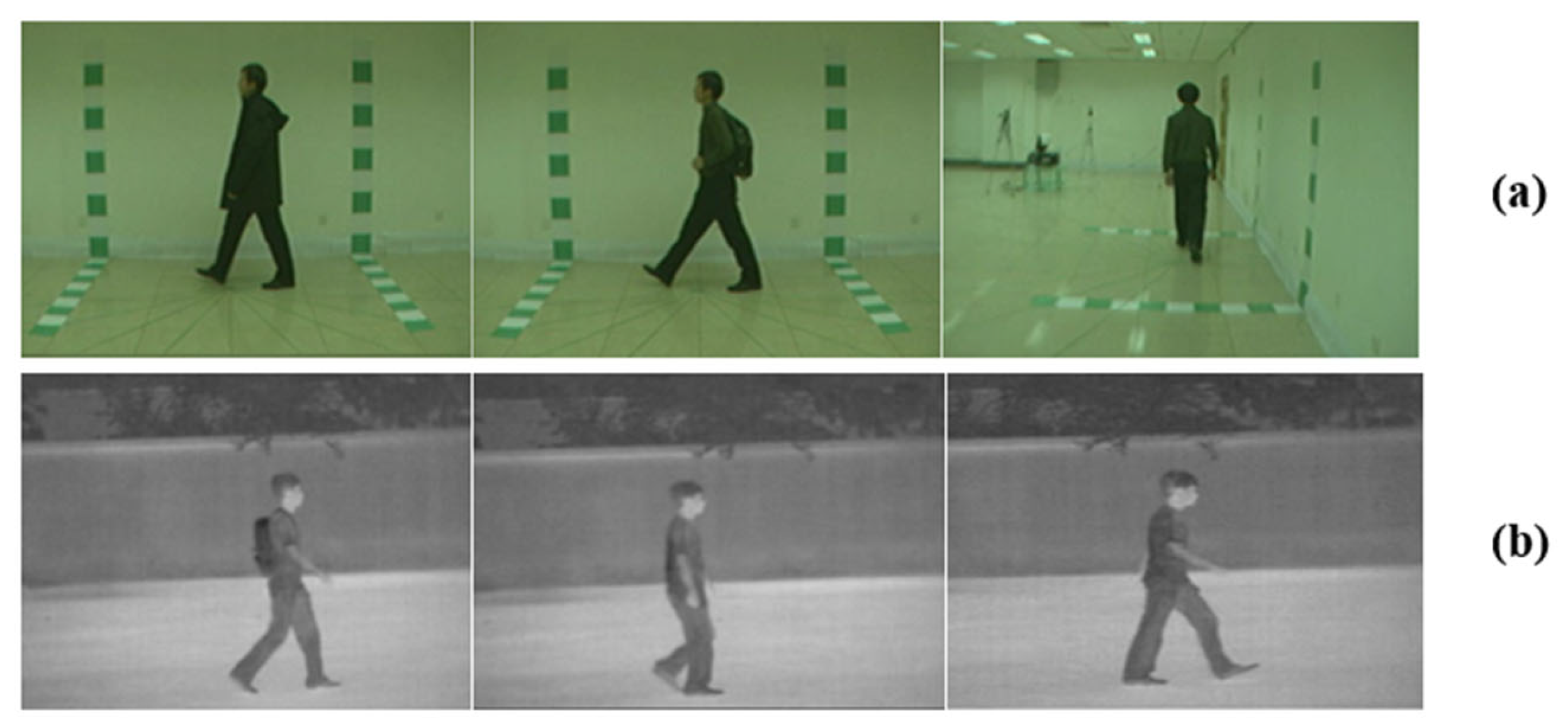
4.1. Datasets

As shown in Figure 5, the CASIA-B dataset includes 124 objects that are in three different walking conditions, including normal (NM), bag (BG), and wearing a coat (CL), containing 11 views from 0° to 180°. The first 62 subjects are used as the training set, and the remaining 62 subjects are used for testing. Specifically, each subject’s first 4 normal walking sequences are used as the gallery set, and the others as the probe set.

CASIA-C is a dataset that contains 153 subjects in different conditions, including normal walking (NW), slow walking (SW), fast walking (FW), and walking with a bag (BW), as shown in Figure 5. Every subject has four NW sequences, two SW sequences, two FW sequences, and two BW sequences. We use the first 24, 62, and 100 subjects as the training set and the last 53 subjects as the testing set. For every subject, NW sequences are used as the gallery set, and the remaining sequences are used as the probe set.

4.2. Comparisons with Other Methods

The performance of the GOFN is compared with other methods on CASIA-B and CASIA-C. As shown in

Table 1. Comparison with previous methods in various views on CASIA-B by accuracies (%), excluding identical-view cases. GOFN obtains the best average results under NM.

Model	NM#5-6	BG#1-2	CL#1-2	Average
SPAE [31]	59.3	37.2	24.2	40.2
MGAN [32]	68.1	54.7	31.5	51.4
Gaitset [9]	92.0	84.3	62.5	79.6
Gait-D [33]	91.6	79.0	72.0	80.9
GaitPart [14]	96.2	92.4	78.7	89.1
GaitGL [15]	95.9	92.1	78.2	88.7
GaitNet [16]	91.5	85.7	58.9	78.7
GaitGraph [21]	87.7	74.8	66.3	76.3
GOFN	96.4	85.5	66.1	82.7

, the experiments show the effectiveness of the GOFN on CASIA-B under cross-view conditions. Our approach achieves an average rank-1 accuracy of 96.4% under normal walking conditions (NM), an accuracy of 85.5% under bag-carrying (BG), and an accuracy of 66.1% under coat-wearing walking (CL) conditions on CASIA-B, excluding identical-view cases. It shows that the accuracy of the GOFN is highest at 144°, and this may be because the spatial and motion features are most abundant in this view. It also indicates that the accuracy under the BG condition is lower than under the NM condition, and the accuracy is the lowest under the CL condition. This may be because the appearances are changed under the BG condition while motion information remains the same, and both spatial and motion features are partly concealed under the CL condition, which brings significant challenges to gait recognition. Compared with the SPAE method proposed by [31] and the MGAN proposed by [32], the GOFN is much more accurate. Compared with Gaitset [9], the accuracy is 4.4% higher on average under NM conditions. Gaitset uses only the silhouette while the GOFI uses both the instantaneous motion information as well as the silhouette edge. The edge of the silhouette in the GOFI retains useful spatial information and is beneficial for accuracy under NM conditions. Moreover, the accuracy is 3.6% higher on average under CL conditions. This may be because the GOFI leverages the motion information, which excludes the influence of the outline of silhouette, and the Set Transition works well. Compared with Gait-D [33] and GaitGraph [21], the methods based on skeleton features, the GOFN performs better under NM and BG conditions, although Gait-D obtains a better result under CL conditions. This may be because skeleton features are free from the errors caused by the coat. Compared with methods using local patterns such as GaitPart [14] and GaitGL [15], the GOFN achieves better results in NM conditions but still encounters issues in BG and CL conditions. However, GaitPart [14] and GaitGL [15] split the original sequence into partitions. In the datasets with aligned subject heights, the methods perform well. But in situations where the heights of subjects change heavily, the methods may encode the misplacement of partitions. However, in our method, the features are extracted from the global silhouettes and the global instantaneous motion, which is more robust when applying the model to subjects with different heights.

As shown in

Table 2. Comparison with previous methods in various views on CASIA-B by accuracy (%) under identical-view conditions. GOFN obtains the best results under BG and CL conditions and remains to be improved under NM conditions.

Probe	Model	0	18	36	54	72	90	108	126	144	162	180	Average
NM#5-6	SPAE [31]	98.4	99.2	97.6	96.0	96.0	96.0	96.8	98.4	97.6	96.8	100.0	97.5
	PoseGait [34]	96.0	96.8	96.0	96.8	96.0	97.6	97.6	94.4	96.8	97.6	97.6	96.6
	LGSD + PSN [35]	99.2	99.2	98.4	99.2	97.6	98.4	97.6	96.8	97.6	97.6	99.2	98.1
	GOFN	98.4	99.2	99.2	97.6	97.6	96.8	96.8	99.2	99.2	98.4	97.6	98.2
BG#1-2	SPAE [31]	79.8	81.5	70.2	66.9	74.2	65.3	62.1	75.8	72.6	68.6	74.2	71.9
	PoseGait [34]	74.2	75.8	77.4	76.6	69.4	70.2	71.0	69.4	74.2	65.3	60.5	71.3
	LGSD + PSN [35]	86.3	84.7	83.1	88.7	90.3	86.3	90.3	83.9	84.7	76.6	80.7	85.0
	GOFN	84.7	88.7	92.7	91.1	85.5	80.7	87.1	88.7	91.9	91.1	79.9	87.5
CL#1-2	SPAE [31]	44.4	49.2	46.8	46.8	49.2	42.5	46.8	43.6	40.3	41.4	42.7	44.9
	PoseGait [34]	46.8	48.4	57.3	61.3	58.1	56.5	59.7	54.8	55.7	58.1	39.5	54.2
	LGSD + PSN [35]	64.5	68.6	70.2	71.0	68.6	64.5	62.9	56.5	59.7	59.7	60.5	64.2
	GOFN	67.7	72.8	77.6	73.4	67.0	67.7	66.1	68.5	69.3	68.5	64.5	69.4

, the experiments show the effectiveness of the GOFN on CASIA-B under the identical-view condition. The performance of the GOFN is compared with other approaches on CASIA-B under identical-view conditions. Under the identical view, the GOFN performs better than other methods. It achieves an accuracy of 98.2% under the NM conditions, 87.5% under the BG conditions, and 69.4% under the CL conditions. Compared with the SPAE method proposed by [28], PoseGait proposed by [34], and LGSD + PSN proposed by [35], the GOFN obtains better performance because the instantaneous motion is less affected under identical-view conditions. Moreover, the GOFN shows its superiority under different conditions, and it exceeds the previous method by at least 2.5% under BG conditions and by at least 5.2% under CL conditions. This shows that the GOFI captured more instantaneous motion using the optical flow, which improves the performance of gait representation. The GOFN used ST and IFP to aggregate the image-level features to set-level features, which helps to exploit the multi-scaled partial features from the GOFIs.

The performance of the GOFN is also evaluated on the CASIA-C dataset with different training sets. As shown in

Table 3. Recognition accuracy (%) under different conditions on CASIA-C with different training sets. Compared with the PSN model, GOFN has better performance under FW and BW conditions.

Training Set	Model	FW	SW	BW	Average
24	LGSD + PSN [35]	58.6	56.0	38.1	50.9
	GOFN	64.2	54.3	39.5	52.7
62	LGSD + PSN [35]	63.6	60.0	42.3	55.3
	GOFN	69.3	58.2	43.5	57.0
100	LGSD + PSN [35]	71.7	71.0	50.5	64.4
	GOFN	76.1	70.5	51.2	67.9

, the GOFN achieves an average accuracy of 51.7% using 24 subjects as the training set, and it achieves accuracies of 56.0% and 64.9% with 62-subject and 100-subject training sets, respectively. This shows that the recognition accuracy increases when the training set is larger. It is because a larger training set has more boundary features, which is beneficial to training the set-level boundaries and reduces overfitting. Moreover, the overall results are lower than those obtained on CASIA-B because the quality of gait sequences in CASIA-C is poorer, introducing outlier data in the process of extracting optical flow. Compared with the PSN proposed by [35], the GOFN increases the accuracy by about 5% under FW conditions and by about 1.8% on average. This may be because the edge of the silhouette in the GOFI, which is helpful spatial information for improving recognition accuracy as motion information may contain outliers under FW conditions, and results under FW conditions are better.

4.3. Ablation Study

The ablation experiments are conducted on the CASIA-B dataset using different components of the GOFN to verify their effectiveness, as shown in

Table 4. Ablation experiments for each structure of GOFN conducted on CASIA-B. Specifically, GEI and GOFI represent different inputs for the network. ST, Max, Mean, Median, and Attention represent different permutation invariant functions to extract set-level features.

Representation		Permutation Invariant Function					IFP	Result
GEI	GOFI	ST	Max	Mean	Median	Attention		NM	BG	CL
√								76.4	64.1	31.8
√		√					√	93.6	85.0	62.2
	√	√					√	96.4	85.5	66.1
	√	√						94.1	82.3	64.7
	√		√				√	92.1	83.8	62.0
	√			√			√	86.5	75.2	48.3
	√				√		√	86.1	74.8	41.1
	√					√	√	91.8	83.3	63.0

. The first row shows the baseline using the GEI directly for classification. The second row shows the results using ST and IFP with the GEI as input, where the result increases by about 20% in NM and BG conditions and about 35% in CL conditions. The third row shows the effectiveness of the GOFI, compared with the GEI; using the GOFI increased the accuracy by 2.8% under NM, 0.5% under BG, and 3.9% under CL conditions. Rows 4–8 show the impact of different components of the GOFN, which demonstrates the effectiveness of ST and IFP.

For the permutation invariant function, it is proven that using ST achieves the highest accuracy compared with other common permutation invariant functions such as max, mean, median, and attention. The ablation experiments show that IFP helps for accuracy as well. With IFP, the result increases by about 2–3% in each condition. Meanwhile, the ablation experiments for the loss function on CASIA-B are shown in

Table 5. Ablation experiments for different loss functions on CASIA-B. The combined loss function performs better than any function alone.

Loss Function	NM	BG	CL
Softmax	31.9	27.9	11.8
Triplet loss	94.2	83.1	62.5
Combined loss	96.4	85.5	66.1

. The outcomes indicate that the combined loss function performs better than any function alone.

5. Conclusions

In this paper, since many methods concern the long-term motion of gait but ignore the short-term motion of gait, a novel GOFI gait representation is proposed to extract the instantaneous motion as well as the silhouette’s edge. Then, the gait features are extracted by the GOFN, which contains an ST architecture to aggregate the image-level features to the set-level features and an IFP to exploit the multi-scaled partial features. The experiments and comparisons conducted on the CASIA-B and the CASIA-C gait datasets show that the GOFN achieves better performances than previous methods under both the cross-view condition and the identical-view condition, which proves the advantages of the GOFN. Moreover, the ablation experiments prove that the GOFI is more effective than the GEI and that the ST and IFP components are also have important impacts on the accuracy of gait recognition. In the future, it will be a very interesting research area to explore the use of walking habits for recognition, since walking habits can be used to theoretically explain the connection between identity and gait.

References

- Lee, T.K.; Belkhatir, M.; Sanei, S. A Comprehensive Review of Past and Present Vision-Based Techniques for Gait Recognition. Multimed. Tools Appl. 2014, 72, 2833–2869. [Google Scholar] [CrossRef]
- Han, J.; Bhanu, B. Individual Recognition Using Gait Energy Image. IEEE Trans. Pattern Anal. Mach. Intell. 2006, 28, 316–322. [Google Scholar] [CrossRef] [PubMed]
- Liu, J.; Zheng, N. Gait History Image: A Novel Temporal Template for Gait Recognition. In Proceedings of the 2007 IEEE International Conference on Multimedia and Expo, Beijing, China, 2–5 July 2007; pp. 663–666. [Google Scholar]
- Chen, C.; Liang, J.; Zhao, H.; Hu, H.; Tian, J. Frame Difference Energy Image for Gait Recognition with Incomplete Silhouettes. Pattern Recognit. Lett. 2009, 30, 977–984. [Google Scholar] [CrossRef]
- Zhang, E.; Zhao, Y.; Xiong, W. Active Energy Image plus 2DLPP for Gait Recognition. Signal Process. 2010, 90, 2295–2302. [Google Scholar] [CrossRef]
- Ji, S.; Xu, W.; Yang, M.; Yu, K. 3D Convolutional Neural Networks for Human Action Recognition. IEEE Trans. Pattern Anal. Mach. Intell. 2013, 35, 221–231. [Google Scholar] [CrossRef] [PubMed]
- Wolf, T.; Babaee, M.; Rigoll, G. Multi-View Gait Recognition Using 3D Convolutional Neural Networks. In Proceedings of the 2016 IEEE International Conference on Image Processing (ICIP), Phoenix, AZ, USA, 25–28 September 2016; pp. 4165–4169. [Google Scholar]
- Qi, C.R.; Su, H.; Mo, K.; Guibas, L.J. Pointnet: Deep learning on point sets for 3d classification and segmentation. In Proceedings of the IEEE Conference on Computer Vision and Pattern Recognition (CVPR), Honolulu, HI, USA, 21–26 July 2017; pp. 77–85. [Google Scholar]
- Chao, H.; He, Y.; Zhang, J.; Feng, J. GaitSet: Regarding Gait as a Set for Cross-View Gait Recognition. In Proceedings of the AAAI Conference on Artificial Intelligence, Honolulu, HI, USA, 27 January–1 February 2019; Volume 33, pp. 8126–8133. [Google Scholar]
- Bashir, K.; Xiang, T.; Gong, S. Gait Recognition Using Gait Entropy Image. In Proceedings of the 3rd International Conference on Imaging for Crime Detection and Prevention (ICDP 2009), London, UK, 3 December 2009; p. P2. [Google Scholar]
- Kusakunniran, W.; Wu, Q.; Zhang, J.; Ma, Y.; Li, H. A New View-Invariant Feature for Cross-View Gait Recognition. IEEE Trans. Inf. Forensics Secur. 2013, 8, 1642–1653. [Google Scholar] [CrossRef]
- Makihara, Y.; Sagawa, R.; Mukaigawa, Y.; Echigo, T.; Yagi, Y. Gait Recognition Using a View Transformation Model in the Frequency Domain. In Proceedings of the 9th European Conference on Computer Vision, Graz, Austria, 7–13 May 2006; Volume 3953, pp. 151–163. [Google Scholar]
- Wang, C.; Zhang, J.; Wang, L.; Pu, J.; Yuan, X. Human Identification Using Temporal Information Preserving Gait Template. IEEE Trans. Pattern Anal. Mach. Intell. 2012, 34, 2164–2176. [Google Scholar] [CrossRef] [PubMed]
- Fan, C.; Peng, Y.; Cao, C.; Liu, X.; Hou, S.; Chi, J.; Huang, Y.; Li, Q.; He, Z. GaitPart: Temporal Part-based Model for Gait Recognition. In Proceedings of the IEEE/CVF Conference on Computer Vision and Pattern Recognition, Seattle, WA, USA, 13–19 June 2020; pp. 14213–14221. [Google Scholar]
- Lin, B.; Zhang, S.; Yu, X. Gait recognition via effective global-local feature representation and local temporal aggregation. In Proceedings of the IEEE/CVF International Conference on Computer Vision 2021, Montreal, BC, Canada, 11–17 October 2021; pp. 14648–14656. [Google Scholar]
- Li, X.; Makihara, Y.; Xu, C.; Yagi, Y.; Ren, M. Gait Recognition via Semi-supervised Disentangled Representation Learning to Identity and Covariate Features. In Proceedings of the IEEE/CVF Conference on Computer Vision and Pattern Recognition, Seattle, WA, USA, 13–19 June 2020; pp. 13306–13316. [Google Scholar]
- Fan, C.; Liang, J.; Shen, C.; Hou, S.; Huang, Y.; Yu, S. OpenGait: Revisiting Gait Recognition Toward Better Practicality. In Proceedings of the IEEE/CVF Conference on Computer Vision and Pattern Recognition, Vancouver, BC, Canada, 18–22 June 2023. [Google Scholar]
- Ariyanto, G.; Nixon, M.S. Model-Based 3D Gait Biometrics. In Proceedings of the 2011 International Joint Conference on Biometrics (IJCB), Washington, DC, USA, 11–13 October 2011; pp. 1–7. [Google Scholar]
- Bodor, R.; Drenner, A.; Fehr, D.; Masoud, O.; Papanikolopoulos, N. View-Independent Human Motion Classification Using Image-Based Reconstruction. Image Vis. Comput. 2009, 27, 1194–1206. [Google Scholar] [CrossRef]
- Kusakunniran, W.; Wu, Q.; Li, H.; Zhang, J. Multiple Views Gait Recognition Using View Transformation Model Based on Optimized Gait Energy Image. In Proceedings of the 2009 IEEE 12th International Conference on Computer Vision Workshops, ICCV Workshops, Kyoto, Japan, 27 September–4 October 2009; pp. 1058–1064. [Google Scholar]
- Teepe, T.; Khan, A.; Gilg, J.; Herzog, F.; Hörmann, S.; Rigoll, G. Gaitgraph: Graph Convolutional Network for Skeleton-Based Gait Recognition. In Proceedings of the 2021 IEEE International Conference on Image Processing (ICIP), Anchorage, AK, USA, 19–22 September 2021; pp. 2314–2318. [Google Scholar]
- Hou, S.; Cao, C.; Liu, X.; Huang, Y. Gait Lateral Network: Learning Discriminative and Compact Representations for Gait Recognition. In Proceedings of the 16th European Conference, Glasgow, UK, 23–28 August 2020; Lecture Notes in Computer Science. Volume 12354, pp. 382–398. [Google Scholar]
- Sepas-Moghaddam, A.; Etemad, A. View-Invariant Gait Recognition With Attentive Recurrent Learning of Partial Representations. IEEE Trans. Biom. Behav. Identity Sci. 2021, 3, 124–137. [Google Scholar] [CrossRef]
- Lucas, B.D.; Kanade, T. An iterative image registration technique with an application to stereo vision. In Proceedings of the IJCAI’81: 7th International Joint Conference on Artificial Intelligence, Vancouver, BC, Canada, 24–28 August 1981; Volume 2, pp. 674–679. [Google Scholar]
- Farnebäck, G. Two-Frame Motion Estimation Based on Polynomial Expansion. In Image Analysis: Proceedings of the 13th Scandinavian Conference, SCIA 2003, Halmstad, Sweden, 29 June–2 July 2003; Lecture Notes in Computer Science; Springer: Berlin/Heidelberg, Germany, 2003; Volume 2749, pp. 363–370. [Google Scholar]
- Simonyan, K.; Zisserman, A. Two-stream convolutional networks for action recognition in videos. Adv. Neural Inf. Process. Syst. 2014, 27, 568–576. [Google Scholar]
- Feichtenhofer, C.; Pinz, A.; Zisserman, A. Convolutional Two-Stream Network Fusion for Video Action Recognition. In Proceedings of the 2016 IEEE Conference on Computer Vision and Pattern Recognition (CVPR), Las Vegas, NV, USA, 27–30 June 2016; pp. 1933–1941. [Google Scholar]
- Luo, Z.; Yang, T.; Liu, Y. Gait Optical Flow Image Decomposition for Human Recognition. In Proceedings of the 2016 IEEE Information Technology, Networking, Electronic and Automation Control Conference, Chongqing, China, 20–22 May 2016; pp. 581–586. [Google Scholar]
- Yu, S.; Tan, D.; Tan, T. A Framework for Evaluating the Effect of View Angle, Clothing and Carrying Condition on Gait Recognition. In Proceedings of the 18th International Conference on Pattern Recognition (ICPR’06), Hong Kong, China, 20–24 August 2006; Volume 4, pp. 441–444. [Google Scholar]
- Tan, D.; Huang, K.; Yu, S.; Tan, T. Efficient Night Gait Recognition Based on Template Matching. In Proceedings of the 18th International Conference on Pattern Recognition (ICPR’06), Hong Kong, China, 20–24 August 2006; Volume 3, pp. 1000–1003. [Google Scholar]
- Yu, S.; Chen, H.; Wang, Q.; Shen, L.; Huang, Y. Invariant Feature Extraction for Gait Recognition Using Only One Uniform Model. Neurocomputing 2017, 239, 81–93. [Google Scholar] [CrossRef]
- He, Y.; Zhang, J.; Shan, H.; Wang, L. Multi-Task GANs for View-Specific Feature Learning in Gait Recognition. IEEE Trans. Inf. Forensics Secur. 2019, 14, 102–113. [Google Scholar] [CrossRef]
- Gao, S.; Yun, J.; Zhao, Y.; Liu, L. Gait-D: Skeleton-Based Gait Feature Decomposition for Gait Recognition. IET Comput. Vis. 2022, 16, 111–125. [Google Scholar] [CrossRef]
- Liao, R.; Yu, S.; An, W.; Huang, Y. A Model-Based Gait Recognition Method with Body Pose and Human Prior Knowledge. Pattern Recognit. 2020, 98, 107069. [Google Scholar] [CrossRef]
- Xu, K.; Jiang, X.; Sun, T. Gait Recognition Based on Local Graphical Skeleton Descriptor With Pairwise Similarity Network. IEEE Trans. Multimed. 2022, 24, 3265–3275. [Google Scholar] [CrossRef]