Robust Full-Screen Wavelength Calibration Algorithm

Abstract

In spectrometer measurement, it is very important to accurately calibrate the wavelength of all target characteristic spectra. Although wavelength calibration methods have long been investigated, no techniques have been designed for the scanning, double-layer, secondary diffraction, linear-array CCD spectrometer, to the best of our knowledge. Based on the grating diffraction equation and experimental results, a mathematical model of wavelength calibration was established for the scanning, double-layer, secondary diffraction, linear-array CCD spectrometer. In this study, a robust, full-screen, wavelength calibration algorithm is proposed, based on the related working principle and the requirements of both accuracy and robustness. The detailed steps are as follows. First, we established a wavelength calibration model at central pixels, following the grating diffraction equation. Then, according to the relationship between the difference in pixels and the feedback values of the grating ruler, a model was established to show the association between these factors. Finally, we combined the two models and built a full-screen wavelength calibration model. We theoretically and experimentally demonstrate that the proposed calibration algorithm is an excellent calibration tool, which can conveniently and accurately calibrate the wavelengths of central and non-central pixels at the same time.

1. Introduction

The spectroscopy applications of spectral analysis methods have been widely used in physics, chemistry, metallurgy, agriculture, environmental protection, building materials, and medicine and health departments. The grating spectrometer is an instrument that uses a beam-splitting element grating to decompose incident composite light into monochromatic light with a narrow spectra [1]. If matched with the corresponding light source and receiving system, the corresponding spectrometer can be formed, which can carry out a spectral analysis of the composite light source. In the meantime, a qualitative and quantitative analysis of transparent substances and solutions can be conducted [2]. The wavelength accuracy refers to the degree of conformity between the wavelength displayed by the instrument and the wavelength of monochromatic light output by the splitting system. The wavelength accuracy is an important metric by which to evaluate the performance of spectrometers. Considering the wavelength accuracy and wavelength repeated-measurement accuracy of the existing near-infrared (NIR) spectrometers, we set the wavelength accuracy of our spectrometer to ±0.05 nm, and the wavelength repeated-measurement accuracy to 0.005 nm. Due to the influence of many factors, such as inherent instrument error and operation mistakes, the wavelength accuracy often cannot meet the applications’ requirements. Therefore, the calibration of grating spectrometers is an indispensable process [3].

Many calibration methods have been developed for the calibration of NIR spectrometers. The polynomial is often used as the fitting curve in the wavelength calibration of central pixels, which can ensure accuracy near the fitting points, but there may be a large gap in the accuracy of the other points [4]. Zhang et al. [5] proposed a simple, laser, wavelength calibration technique based on the second harmonic signals to improve the performance of a quartz-enhanced photoacoustic spectroscopy (QEPAS) gas-sensing system. Sun et al. [6] employed the peak method and gravity method to calibrate the wavelength of the prism-grating imaging spectrometer. This work shows that the difference between the two calibration results is within 0.3 nm. The gravity method was found to be insensitive to spot energy mutations, and can effectively improve the efficiency and accuracy of wavelength calibration. Moreover, some researchers also proposed wavelength calibration algorithms for laser spectral measurements based on cubic spline interpolation and the kernel regression method [7].

Research on robust calibration has also attracted much attention. Mark and Workman [8] proposed a method to calibrate wavelength offset using multiple regression equations, which can make the calibration robust. Swierenga et al. [9] used robust wavelength selection to make the calibration robust to more general forms of between-instrument variation.

At present, wavelength calibration methods are mainly used for the following two kinds of spectrometer.

1.

At present, calibration methods are mostly used for spectrometers with a fixed grating. This type of spectrometer is commonly characterized by the small line-pairs grating and linear-array CCD. Spectrometers with this structure tend to have a lower wavelength calibration accuracy and a lower spectral resolution.

2.

For the grating rotational spectrometer, a single-element detector and large line-pairs grating are usually used.

However, there is no suitable wavelength calibration method for spectrometers using linear-array CCD and rotational grating with large line pairs. To solve the problems with the existing technology, a wavelength calibration method for the scanning, double-layer, secondary-diffraction, linear-array CCD spectrometer is proposed in this study.

In this study, we propose a novel wavelength calibration method for this type of spectrometer. The main contributions of our work are summarized as follows.

1.

At the central pixels, we use the Levenberg–Marquardt algorithm to correct the function relationship between wavelength and feedback value and obtain a sinusoidal function.

2.

We creatively propose converting the feedback values of the non-central pixels into its corresponding feedback values at the central pixels, and then calculate the wavelength using the formula in the previous step. Based on the linear relationship between wavelengths and feedback values, the Huber regression is employed to fit a robust model to better overcome the inherent instrument errors and operation mistakes.

3.

By integrating the formulas obtained in step 1 and step 2, we obtain a wavelength calibration formula that can accurately calibrate all pixels. Experiments show that the novel calibration method has good continuity and high wavelength calibration accuracy.

The rest of this study is organized as follows. Section 2 mainly describes the structure and related principle of the scanning, double-layer, secondary diffraction, linear-array CCD spectrometer. Section 3 describes the detailed calibration algorithm. The performance of the algorithm is verified by some experiments in Section 4. Finally, Section 5 contains the conclusions of the study.

2. Spectrometer Construction and Related Principles

To facilitate later discussions, this section will introduce the optical construction and some basic principles of the scanning, double-layer, secondary diffraction, linear-array CCD spectrometer.

2.1. Construction of the Scanning, Double-Layer, Secondary Diffraction, Linear-Array CCD Spectrometer

The wavelength calibration method of the scanning, double-layer, secondary diffraction, linear-array CCD spectrometer is suitable for the high-precision spectrometer with a double-layer grating, linear grating ruler, collimating lens (spherical lens), converging lens (aspheric lens), bending mirror, continuous current dynamo, linear-array CCD, raster scanning mechanism, etc. The spectrometer usually includes an optical path module, an integrated control module, a signal acquisition and processing module, and a portable industrial computer.

In the optical path module, as demonstrated in Figure 1, the components numbered from 1 to 10 represent the filter, incident slit, shutter, spherical lens, grating group 1, plane mirror 1, plane mirror 2, grating group 2, aspheric lens, and linear CCD, respectively. Figure 1 clearly shows how an incident light propagates inside the spectrometer. Here, the red and blue lines indicate the upper and lower layers of the optical path, respectively.

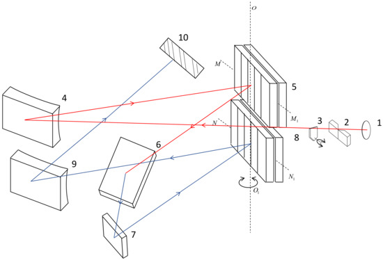
Figure 1. The optical layout of the discussed spectrometer.

The integrated control module mainly includes a power supply, slit control module, filter control module, grating group control module, and rotating mirror control module. The signal acquisition and processing module is a high-speed acquisition and processing circuit of a linear-array CCD. The portable industrial computer is the sender of the received instruction, and the receiver of the feedback signal of the integrated control module, as well as the the signal-receiver of the signal acquisition and processing module.

The double-layer grating comprises four gratings, and each group of two gratings has the same number of lines. Grating group 1 and grating group 2 were placed with a 1200-line grating and 2400-line grating, respectively, back-to-back and in parallel. Grating group 1 and grating group 2 were rotated in a common axis. Both 1200-line grating group 1 and 1200-line grating group 2, and 2400-line grating group 1 and 2400-line grating group 2, were simultaneously used for optimal path diffraction. The two groups of gratings were placed at the top and bottom of a plane. The upper and lower gratings with the same number of lines formed a group of dispersion units, and each group of dispersion units was installed on the same scanning rotation axis. The spectrometer has a sine mechanism. The linear grating ruler was installed on the linear guide rail, and the reading head was installed on the sinusoidal rod. The purpose was to feedback the rotation position of the grating and monitor the accuracy of the raster scanning positioning. The detector was a linear-array, charge-coupled device (CCD), with a pixel number of $2048\times 1$. By processing of signal acquisition and the processing module, we obtained the wavelength map spread with 2048 pixels in the upper computer. The 1024$th$ pixel is called the central pixel and the rest are called non-central pixels.

Typical light sources include mercury lamps and lasers. When the shutter is opened during measurement, the light emitted by the light source passes through the filter to filter out the secondary spectrum, and the slit width is adjusted so that there is a good match between the useful signal received by the spectrometer and the spectral resolution. After that, the light passes through a spherical lens and the diverging light is collimated to parallel light. Parallel rays are split through grating group 1, and the rays of different wavelengths are reflected in plane mirror 1 at a certain angle. After being processed by plane mirror 1 and plane mirror 2, the upper optical path is transferred to the lower optical path. The light reflected by the plane mirror groups passes through grating group 2, and is split twice by grating group 2. Light rays of different wavelengths are reflected in the aspheric lens at twice the angle of the corresponding wavelength of grating 1. This grating group 2 operation improves the spectral resolution of the spectrometer. Through the aspheric lens, the parallel light of different angles of incidence is imaged into the linear-array CCD.

The characteristic peaks in the mercury lamp are 253.65 nm, 312.57 nm, 365.02 nm, 404.66 nm, 435.84 nm, 546.07 nm, 576.96 nm, and 570.07 nm. According to these wavelengths, the wavelengths of 2048 pixels can be calibrated using the wavelength calibration algorithm proposed in this paper. In addition to achieving better calibration accuracy at the provided fitting points, it can also calibrate the wavelengths at other points. In this paper, the spectral range of the spectrometer is 200–1000 nm, and the spectral range of the 2400-line grating is 200–650 nm.

2.2. Theoretical Background

Based on the optical theory, we set out to establish the wavelength calibration model for the central pixels in the linear-array CCD [10]. Theoretically, the grating diffraction equation is

$$m\lambda =d(\sin {\omega }_1-\sin {\omega }_2),$$

(1)

where d is the grating line spacing, ${\omega }_1$, and ${\omega }_2$ are the incidence angle and diffraction angle of the relative grating normal, respectively. m is the order of the diffraction spectrum, and $\lambda$ is the wavelength of the diffraction light. In addition, the diffraction order is set as level 1.

In order to simplify the calibration process, we designed a grating sine mechanism for the spectrometer. By applying the differential product transformation of trigonometric functions to Equation (1), and setting $({\omega }_1+{\omega }_2)/2={\tau }_1$ and $({\omega }_1-{\omega }_2)/2={\tau }_2$, the dispersion equation can be expressed as

$$\lambda =2d\cos {\tau }_1\sin {\tau }_2.$$

(2)

In the test instrument, ${\tau }_1$ is a fixed value. ${\tau }_2$ represents the rotation angle of the grating; that is, the rotation angle when the grating scans to a certain diffraction light wavelength, starting from the alignment of zero-order light.

Assuming that the length of the sinusoidal bar is L, the translation distance of the slider is x, i.e., the feedback value, and the angle of the sinusoidal bar is ${\tau }_2$, then the relationship [11] should be

$$x=L\sin {\tau }_2.$$

(3)

As the installation position of the slider is variable, the wavelength and the feedback value of the sine mechanism are related through the formula

$$\lambda =2d\cos {\tau }_1\frac{x}{L}+a.$$

(4)

Equation (4) shows that the linear displacement distance of the sinusoidal machine has a linear relationship with the diffraction wavelength of the grating. This configuration can greatly simplify the central wavelength calibration. However, in the experiment (Section 4.1), we found that linear fitting is not as effective as sinusoidal fitting.

3. The Proposed Calibration Method

As there are high requirements regarding spectrometer accuracy, we have to solve the calibration problem of the scanning, double-layer, secondary diffraction, linear-array CCD spectrometer. The main difficulties that were encounted are as follows. First the spectral wavelength at the central pixels must be accurately determined using the wavelengths obtained from the limited standard light source, and good calibration accuracy must simultaneously be achieved at other wavelengths. Secondly, the wavelength we must be accurately calculated at the non-central pixels, while simultaneously making the algorithm robust. Finally, a continuous algorithm that can simultaneously calibrate all pixels should be generated.

After analyzing the working principles of a spectrometer and the causes of the above-mentioned difficulties, we propose the following calibration algorithm. First, the wavelengths of the center pixels are calibrated. According to Equation (4), we conducted a rough calibration, obtained the data pairs needed for the subsequent accurate calibration, and then corrected them using our algorithm’s sinusoidal function. Then, when the feature peak of the wavelength reached the non-central pixel, the feedback value of the grating ruler (feedback value) of the central pixel was recorded. To convert the feedback value recorded at the central pixel when the wavelength reaches the non-central pixel into the feedback value of the wavelength at the central pixel, the functional relationship between the pixel’s difference and the feedback value is established. Finally, the spectral wavelength calibration algorithm of full-screen pixels was presented by integrating the previous two steps.

It should be noted that the 1200-line grating of this spectrometer has a spectral range from 200 nm to 1000 nm, and the 2400-line grating has a spectral range from 200 nm to 650 nm. Without loss of generality, we use the 2400-line grating as an example in our discussion. The calibration method can be directly applied to the 1200-line grating.

3.1. Spectral Wavelength Calibration Algorithm at Central Pixels

We used the wavelengths of standard light sources (i.e., mercury lamps and lasers) to calibrate the spectrometer. The linear model obtained in Equation (4) was used for the rough calibration of wavelength (please refer to Appendix A.1 for a detailed introduction). We can obtain data pairs for the central pixels that we need using rough calibration. Through experiments, we designed a sinusoidal model, using the Levenberg–Marquardt algorithm (LMA) to correct the wavelength calibration. The new model is better than the model constructed in Equation (4). Through this model, a sinusoidal curve is obtained to predict the relationship between wavelengths other than standard wavelengths, and the corresponding feedback values.

The Levenberg–Marquardt Algorithm to Fit the Sinusoidal Function

To implement accurate calibration, we require more feedback value and wavelength data pairs. With the method described in Appendix A.1, we can obtain data pairs ($x_c^1,{\lambda }_c^1$), ⋯, ($x_c^n,{\lambda }_c^n$) at central pixels.

According to the results of the experiment, the sinusoidal model is more realistic than the linear model. Assume that the relationship can be represented as

$${\lambda }_c=a\sin (b{x}_c+c)+d,$$

(5)

where $x_c\left({[x_c^1,x_c^2,\cdots ,x_c^n]}^{\top }\right)$ and ${\lambda }_c\left({[{\lambda }_c^1,{\lambda }_c^2,\cdots ,{\lambda }_c^n]}^{\top }\right)$ are the feedback value and wavelength at the central pixel, respectively. $a,b,c,d$ are unknown parameters. To simplify discussions, we denote $\theta =[a,b,c,d]$.

Suppose the fitting non-linear function to be $f(X\mid \theta ),$ and the initial value of $\theta$ is ${\theta }_0=[a_0,b_0,c_0,d_0]$. Therefore, we can find the optimal values for $\theta$ by minimizing

$$F\left(\theta \right)=\sum _{i=1}^n{(f(x_c^i\mid \theta )-{\lambda }_c^i)}^2=f{\left(\theta \right)}^{\top }f\left(\theta \right),f(x_c^i\mid \theta )=a\sin (b{x}_c^i+c)+d,$$

(6)

where $f\left(\theta \right)=f(x_c\mid \theta )-{\lambda }_c$. As this is a non-linear, least-square problem, the LMA is used to provide a solution.

The LMA is based on the trust region theory because the Taylor expansion in the Gauss–Newton method can only have a good effect near the expansion points. Therefore, to ensure approximation accuracy, we need to set a region with a certain radius as the trust region. In LMA, the size of the trust region is determined by the gain ratio, which is defined as

$$\rho =\frac{f(\theta +\Delta \theta )-f\left(\theta \right)}{J{\left(\theta \right)}^{\top }\Delta \theta },$$

(7)

where $J\left(\theta \right)$ is $f{\left(\theta \right)}^{\prime }$.

3.2. Functional Relation at Non-Central Pixels

After obtaining the optimal $\theta$ by Algorithm 1, Equation (5) can be established and the wavelengths at central pixels can be considered accurately calibrated. However, for the non-central pixels, further processing is required. Notice that, in the actual operation of the spectrometer, outliers often occur due to inherent instrument error or operation mistakes, which inevitably affect the performance of the calibration algorithm. As a result, it is necessary to make the algorithm robust to outliers while maintaining a high wavelength accuracy. As the Huber regression and Turkey regression are robust to outliers (the detailed argument is presented in Section 3.2.1 and Section 3.2.2), we compare the performance of Huber regression, Tukey regression, and least squares regression methods with the collected experimental data, so that a more suitable approach can be found. We also tried some other robust regression methods, such as RANSAC regression and Theil Sen regression. However, we found that they performed a little worse than Huber regression (the detailed argument is presented in Section 4.1). To simplify this paper, other robust regression algorithms are not listed.

In this part, the data were collected as described in Appendix A.2.1 of the Appendix A. We divide the data into two cases: central pixels ($x_c$, $p_c$) and non-central pixels ($x_n$, $p_n$). For the standard wavelength ${\lambda }_c$, we first performed a preliminary analysis with $\Delta x=x_n-x_c$, $\Delta p=p_n-p_c$. The $p_n$ value ranges from 1 to 2048. By exploring the scatter plot of $\Delta x$ and $\Delta p$, as shown in Figure 2, a linear relationship between them is demonstrated. According to this fact, we will fit a linear regression model.

Algorithm 1 The Levenberg–Marquardt method used to fit the sinusoidal function at central pixels

Input:n datapoints ($x_c^1,{\lambda }_c^1$), ⋯, ($x_c^n,{\lambda }_c^n$), the initial weight ${\theta }_0$, and the initial optimization radius $u_0$. Output: The optimal $\theta$.   1: Let $k=1$.   2: while$k<\mathrm{50,000}$ and $F\left({\theta }_k\right)>1.5\times {10}^{-8}$ and $\parallel {\theta }_k-{\theta }_{k-1}{\parallel }_1>1.5\times {10}^{-8}$ do   3:    Use the Gaussian–Newton method and the trust region to solve     $mi{n}_{\Delta {\theta }_k}\frac{1}{2}\Vert f\left({\theta }_k\right)+J{\left({\theta }_k\right)}^{\top }\Delta {\theta }_k{\Vert }^2,s.t.{\Vert \Delta {\theta }_k\Vert }^2\le u_k$    where $u_k$ is the radius of the trust region, $J\left({\theta }_k\right)$ is the Jacobian matrix of the function.   4:    Based on the obtained $\Delta {\theta }_k$, calculate $\rho$ according to Equation (7).    If $\rho \ge \frac{3}{4}$, let $u_{k+1}=2u_k$.    If $\rho \le \frac{1}{4}$, let $u_{k+1}=0.5u_k$.    If $\frac{1}{4}<\rho <\frac{3}{4}$, $u_{k+1}=u_k$.    If $\rho <0$, ${\theta }_{k+1}={\theta }_k,u_{k+1}=0.5u_k$. However, the    ${\theta }_{k+1}={\theta }_k+\Delta {\theta }_k$.   5:    $k=k+1$.   6: end while   7: return  $\theta$

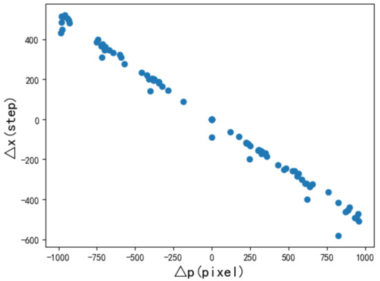
Figure 2. The scatter plot of $\Delta x$ and $\Delta p$.

Suppose that the model between $\Delta x$ and $\Delta p$ is

$$\Delta x=e\Delta p+f+\epsilon ,$$

(8)

where $\Delta x$ and $\Delta p$ indicate the response and independent variables, respectively. The symbols e and f are unknown regression parameters, and $\epsilon$ is the random noise term. We denote $\beta =[e,f]$, $f_{\beta }(\Delta p)=\beta {[\Delta p,1]}^{\top }$.

The core idea of our proposed non-central pixel algorithm is to estimate the feedback value $x_c$ when the feature peak ${\lambda }_c$ is at the non-central pixel $p_n$ according to the established Equation (8), given the known values of $p_c$, $p_n$ and $x_n$. In other words, $x_n$ at $p_n$ can be converted to $x_c$ at $p_c$ by Equation (8). Since the wavelength of the central pixel $p_c$ was accurately calibrated by Equation (5), the wavelength of the non-central pixel can be calibrated by the feedback value $x_c$ estimated using the above procedure. By this means, we calibrated the wavelengths of the non-central pixels.

3.2.1. Huber Regression

As previous analysis has shown that a linear relationship exists between $\Delta x$ and $\Delta p$, we studied the least-square method (LS) method and robust regression methods, including Huber and Turkey regression models.

Some observed data $(\Delta x_i,\Delta p_i)(i=1,2,\cdots ,N)$ can be used to denote the residuals by $r_i=f_{\beta }(\Delta p_i)-\Delta x_i$, in which $f_{\beta }(\Delta p_i)$ denotes the value fitted by a linear regression model with $\beta$.

As the wavelength calibration requires both robustness and accuracy, the Huber regression [12,13] was adopted to fit the model. By defining

$$\rho \left(r_i\right)=\left\{\begin{array}{cc}{r}_i^2/2,\hfill & |r_i|\le \eta \hfill \\ \eta |r_i|-{\eta }^2/2,\hfill & |r_i|>\eta \hfill \end{array}\right.$$

(9)

where $\eta$ is a pre-specified threshold value. The objective is to minimize

$$\widehat{\beta }=\underset{\beta }{\mathrm{argmin}}L\left(\beta \right),L\left(\beta \right)=\sum _{i=1}^n\rho \left(r_i\right).$$

(10)

By defining $\varphi \left(r_i\right)={\rho }^{\prime }\left(r_i\right)$, Huber’s influence function is

$$\varphi \left(r_i\right)=\left\{\begin{array}{cc}{r}_i,\hfill & |r_i|\le \eta \hfill \\ \mathrm{sgn}\left(r_i\right)\eta ,\hfill & |r_i|>\eta \hfill \end{array}\right.$$

(11)

According to the definition, the influence function reflects the influence of $\Delta p_i$ on the gradient. By setting $\psi \left(r_i\right)=\varphi \left(r_i\right)/r_i$, Huber’s weight function can be expressed as

$$\psi \left(r_i\right)=\frac{\varphi \left(r_i\right)}{r_i}=\left\{\begin{array}{cc}1,\hfill & |r_i|\le \eta \hfill \\ \eta /|r_i|,\hfill & |r_i|>\eta \hfill \end{array}\right.$$

(12)

In other words, when $|r_i|$ is larger than the hyperparameter $\eta$, the corresponding $\Delta p_i$ is judged to be an outlier, and its effect is specified as $sgn\left(r_i\right)\eta$. When $|r_i|$ is less than $\eta$, the influence of $\Delta p_i$ is set as $r_i$. We also note that Huber regression has advantages compared to other methods in Appendix A.2.2 of the Appendix A. In comparison with the mean squared error (MSE), Huber’s loss is less sensitive to outliers because their weights are reduced. In comparison with the mean absolute error(MAE), this can converge faster.

The main steps of using Huber regression to calibrate the wavelengths at non-central pixels are listed in Algorithm 2.

Algorithm 2 Spectral wavelength calibration algorithm at noncentral pixels

Input: The step size $l{r}_0$, the initial weight vector ${\beta }_0$, the hyperparameter $\eta$, the number of iterations E, the initial value of the first-order differential $D_0$, the data pairs $(\Delta x_i,\Delta p_i)(i=1,2,\cdots ,N)$ Output: The final estimated parametric vector $\beta$ 1: for  $j=1,2,\cdots ,E$  do 2:    for $k=1,2,\cdots ,N$ do 3:      $\Delta x_k^{pred}={\beta }_k{[\Delta p_k,1]}^{\top }$ 4:      if $\mid \Delta x_k-\Delta x_k^{pred}\mid \le \eta$ then 5:         ${\psi }_k=1$ 6:      else 7:         ${\psi }_k=\frac{\eta }{\mid \Delta x_k-\Delta x_k^{pred}\mid }$ 8:      end if 9:      $D_k=D_{k-1}-{\psi }_k{[\Delta p_k,1]}^{\top }\mid \Delta x_k-\Delta x_k^{pred}\mid$ 10:    end for 11:    ${\beta }_j={\beta }_{j-1}-l{r}_0{D}_k$ 12: end for 13: return  $\beta$

3.2.2. Tukey Regression

Although the influence of outliers is weakened in Huber regression, some extreme outliers still have harmful influences on the final result. To overcome this shortcoming, Turkey [14] proposed defining the function $\rho \left(r_i\right)$ as

$$\rho \left(r_i\right)=\left\{\begin{array}{cc}(1-{[1-{r_i}^2/{\eta }^2]}^3){\eta }^2/6,\hfill & |r_i|\le \eta \hfill \\ {\eta }^2/6,\hfill & |r_i|>\eta \hfill \end{array}\right.$$

(13)

Evidently, Turkey’s loss function $L\left(\beta \right)$ is not a convex function; that is, several local optima may exist. In practice, the following weight function is commonly employed, i.e.,

$$\psi \left(r_i\right)=\left\{\begin{array}{cc}{(1-r_i^2/{\eta }^2)}^2,\hfill & |r_i|\le \eta \hfill \\ 0,\hfill & |r_i|>\eta \hfill \end{array}\right.$$

(14)

Equation (14) shows that outliers no longer have any effect on the estimated $\beta$. The main steps used to fit a regression model with Turkey’s loss function are similar to those shown in Algorithm 2, except that the weight function $\psi \left(r_i\right)$ is replaced with Equation (14).

3.3. Full-Screen Spectral Wavelength Calibration Algorithm

In summary, the relationship between the wavelength ${\lambda }_c$, the feedback value x($x_c$ or $x_n$), and the pixel positions $p_c$ and $p_n$ can be formulated as

$${\lambda }_c=a\sin (b(x-(e(p_n-p_c)+f))+c)+d,$$

(15)

where $a,b,c,d,e$ and f are unknown parameters. Note that x can serve as the feedback value $x_c$ for the standard wavelength ${\lambda }_c$ at the central pixel, and $x_n$ for the standard wavelength ${\lambda }_c$ at the non-central pixel. In other words, Equation (15) can calibrate the wavelengths at central and non-central pixels. It is notable that the difference between Equations (15) and (5) is small when $p_n$ is equal to $p_c$. The difference between the two functions is the initial phase $-bf$. This may result in a loss of calibration accuracy at the central pixels. However, since the magnitude of x in our actual experiment was ten thousand, and the calculated parameters b and f are single digits, the error caused by the initial phase is negligible after verification; therefore, we still used Equation (15) for the continuity of full-screen calibration (without breaking point).

The main steps of full-screen spectral wavelength calibration algorithm are listed in Algorithm 3.

Algorithm 3 Full-screen spectral wavelength calibration algorithm

Input: (${\lambda }_c$, $x_c$, ${x_n}^i$, $p_c$, ${p_n}^i)$, $(i=1,2,\cdots ,N)$, the initial weight ${\theta }_0=[a_0,b_0,c_0,d_0]$, ${\beta }_0=[e_0,f_0]$, the step size $l{r}_0$, the hyperparameter $\eta$, the number of iterations E, the initial value of first-order differential $D_0$. Output: All parameters of Equation (15) 1: According to $x_c$ and the central wavelength ${\lambda }_c$, $\theta$ is calculated by Algorithm 1, where $\theta =[a,b,c,d]$. 2: According to ($x_c$, ${x_n}^i$, $p_c$, ${p_n}^i)$, $i=1,2,\cdots ,N$, Algorithm 2 is used to calculate $\beta$, where $\beta =[e,f]$. 3: Obtain all parameters in Equation (15).

4. Experimental Studies

The proposed method was used to calibrate the wavelength of three scanning, double-layer, secondary diffraction, linear-array CCD spectrometers. The 2400-line grating of grating group 1 and the 2400-line grating of grating group 2 were used when the spectrometer diffracted. The linear-array CCD was a linear-array CCD with a pixel number of 2048 × 1, and the spectral range was 200–650 nm.

4.1. Simulated Experiments

We used wavelength standards 1 and 2 to record the standard wavelength ($x_{01}$, $x_{02}$) and its reading head number (${\lambda }_{01}$, ${\lambda }_{02}$) at the central pixels. Using ($x_{01}$, ${\lambda }_{01}$) and ($x_{02}$, ${\lambda }_{02}$), we can fit Equation (4) using rough calibration, as described in Appendix A.1.

According to Equation (4), the feedback values $x_{10}$, $x_{20}$, $x_{30}$, $x_{40}$, $x_{50}$, $x_{60}$, $x_{70}$, $x_{80}$ of the grating ruler were calculated when the characteristic wavelengths of the mercury lamp were 253.65 nm, 312.57 nm, 365.02 nm, 404.66 nm, 435.84 nm, 546.07 nm, 576.96 nm, and 570.07 nm, respectively. Using the above data pairs, the scanning motor pulse was set so that each feature spectrum scanned to the central pixel of the linear-array CCD. In this way, accurate test results $x_{11}$, $x_{21}$, $x_{31}$, $x_{41}$, $x_{51}$, $x_{61}$, $x_{71}$, $x_{81}$ could be obtained from the feedback values of the grating ruler. With $(x_{11},253.65)$, $(x_{21},312.57)$,$(x_{31},365.02)$,$(x_{41},404.66)$, $(x_{51},435.84)$, $(x_{61},546.07)$, $(x_{71},576.96)$, $(x_{81},570.07)$, we conducted experiments to verify the performance of the central pixel wavelength calibration algorithm (i.e., Algorithm 1).

Specifically, the nonlinear least square method under LMA was used for calculation, and its parameters were initialized, as shown in Table 1, where ${\lambda }_c$ is the characteristic wavelength of the mercury lamp and $freq$ is a given frequency. The reasons the initial values were set in this way, such as the limited space, are explained in Appendix A.3.

Table 1. The initial values of the parameters in Equation (5).

Parameter	${\mathit{a}}_0$	${\mathit{b}}_0$	${\mathit{c}}_0$	${\mathit{d}}_0$
Initial value	$max\left({\lambda }_c\right)-min\left({\lambda }_c\right)$	$2\pi freq$	0	$mean\left({\lambda }_c\right)$

Figure 3 shows the sinusoidal curve fitted by Algorithm 1; the fitted parameters are shown in Table 2. In Figure 3, the horizontal axis indicates the wavelength and the vertical axis is the feedback value. The fitting performance is good, as the known wavelengths and feedback values are fitted very well. By calculation, the maximum difference between the original data and the fitted sinusoidal function was shown to be 0.03365 nm.

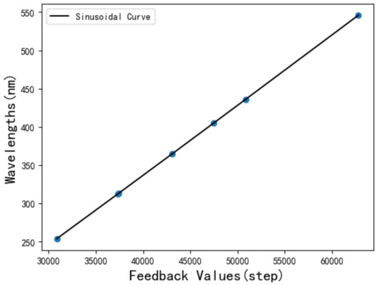
Figure 3. Sinusoidal fitting results of the central pixels.

Table 2. The fitting parameters of Algorithm 1.

Parameter ($\mathit{\theta }$)	a	b	c	d
Fitting results	−1993.820	4.65 $·{10}^{-6}$	2.773	699.383

Next, we simulated some experimental data to validate the performance of the calibration algorithm at non-central pixels. We turned on the mercury lamp and let the light from the mercury lamp that was vertically incident on the light inlet of the spectrometer. The scanning motor was started to rotate the raster scanning machine to 0 nm, and then the raster scanning machine was started. According to the pixel number of linear-array CCD (take 2048 × 1 linear-array CCD as an example), the average value $x_1$, $x_{256}$, $x_{512}$, $x_{768}$, $x_{1280}$, $x_{1536}$, $x_{1792}$, $x_{2048}$ (denoted as X) of the feedback value of the grating ruler corresponding to the feature peak at $p_1$(the first pixel), $p_{256}$, $p_{512}$, $p_{768}$, $p_{1280}$, $p_{1536}$, $p_{1792}$, and $p_{2048}$ (denoted as P) of a certain feature peak were recorded. In a similar way, we also recorded the feedback values X that correspond to the characteristic peaks in the mercury lamp 253.65 nm, 312.57 nm, 365.02 nm, 404.66 nm, 435.84 nm, 546.07 nm, 576.96 nm, 570.07 nm. Based on these data, we used Algorithm 2 to test its performance.

According to Algorithm 2, We selected the initial step size $l{r}_0$, the initial weight ${\beta }_0$, the hyperparameter $\eta$, and the E values within a certain range. The initial step size $l{r}_0$ and the hyperparameter $\eta$ were selected from $\{0.01,0.001,0.0001\}$. The selection range of the initial weight ${\beta }_0$ was one of the intervals from $\left\{\right(-0.1,-0.1),(0,0),(0.1,0.1\left)\right\}$. The candidate values of the epoch number E were set as $\{100,150,200\}$. The final hyperparameter configuration, obtained after conducting some preliminary analyses with different combinations of these hyperparameters, is shown in Table 3.

Table 3. Selected hyperparameters for three fitting methods.

Hyperparameter	${\mathit{lr}}_0$	${\mathit{\beta }}_0$	$\mathit{\eta }$	E	${\mathit{D}}_0$
Value	0.0001	[−0.1, −0.1]	0.001	150	[0, 0]

With data pairs $\Delta x$ and $\Delta p$, we fitted the linear regression model using the LS method, Huber regression, and Turkey regression. The left subplot of Figure 4 shows the fitting results of Huber regression, LS regression, and Tukey regression. The horizontal and vertical axes represent $\Delta p$ and $\Delta x$, respectively. The blue points are the observed data and the lines are the linear models fitted by the three methods. To facilitate comparison, we enlarged the contents of the red box; it is shown in the right subplot. These results reveal that Huber regression performs better than the other methods in resisting outliers. The fitted parameters, obtained according to Huber regression, are shown in Table 4.

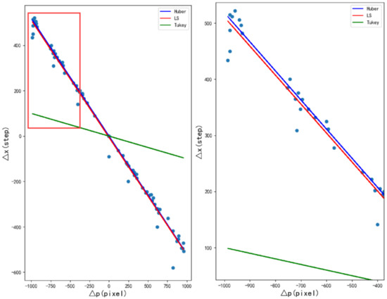
Figure 4. Comparison of the three fitting methods. Note: The blue points are the observed data. The blue, red, and green lines are the Huber, LS, and Tukey regression predictions, respectively. The image on the right is a partial enlargement in the red box on the left.

Table 4. The fitting parameters of Algorithm 2.

Parameter ($\mathit{\beta }$)	e	f
Fitting results	−0.519	−0.0981

To further demonstrate the advantages of Huber regression, we conducted a quantitative analysis of the fitting results. Since Figure 4 shows that Turkey regression works the worst, only LS and Huber regression were taken into account. First, we removed the nine farthest outliers from the linear function obtained using the LS method according to the absolute value of the residuals. Then, the LS RANSAC, Theil Sen, and Huber regression were compared on the remaining points. We computed the mean squared error ($\mathrm{MSE}$), the maximum residual ($\mathrm{RES}$) and the mean absolute error ($\mathrm{MAE}$). Figure 5 demonstrates the obtained results, in which columns 1, 2, and 3 correspond to the MSE, RES, and MAE, respectively. Different colors represent different regression algorithms.

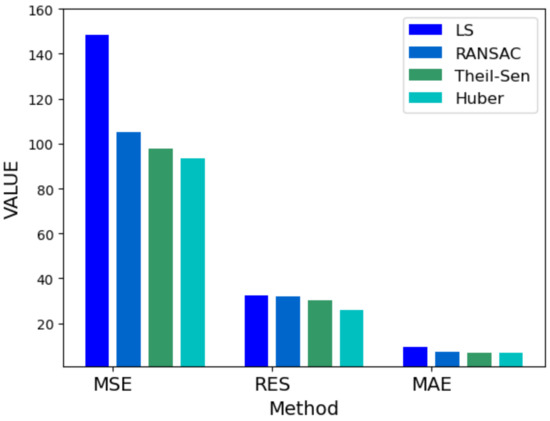
Figure 5. Qualitative comparison between Huber and LS.

Figure 5 shows that Huber regression performs better than LS, RANSAC, and Theil Sen regression in terms of the evaluation indices $\mathrm{MSE}$, $\mathrm{MAE}$ and $\mathrm{RES}$. In industrial practice, the maximum residual error is often chosen as the criterion by which to judge the quality of the algorithm. Therefore, the smaller the $\mathrm{RES}$, the better the algorithm. Based on this fact, we chose the $\widehat{\beta }$ estimated by the Huber method.

4.2. Validation on the Instrument

In this subsection, we qualitatively analyze the calibration algorithm. This is shown in Figure 6, where the horizontal axis indicates the wavelength. On the vertical axis, the left part denotes the signal energy collected by CCD, while the right part denotes the signal voltage value. In Figure 6, the full width at half-maximum (FWHM) reflects the spectral resolution, W represents the wavelength value calibrated by the algorithm, P represents the pixel position, C means the signal energy value collected by the CCD, and V represents the signal voltage value. The units of these values in Figure 6 are nm, nm, pixel, count, and V.

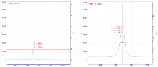
Figure 6. Qualitative analysis of the calibration algorithm. Note: The left vertical axis represents the signal energy value, the right represents the signal voltage value, and the horizontal axis represents the wavelength value calibrated by the algorithm. The center of the red cross in the picture is the wavelength we are measuring, and we usually know the exact value of it. FWHM reflects the spectral resolution, W represents the wavelength value calibrated by the algorithm, P represents the pixel position, C means the signal energy value collected by the CCD, and V represents the signal voltage value.

The left subplot of Figure 6 shows the calibration accuracy of the fitting wavelengths. At the characteristic peak of 404.65 nm, the wavelength after calibration is 404.696 nm. The calibration accuracy at this pixel is 0.046 nm, and the spectral resolution is 0.016 nm. This shows that the calibration algorithm can achieve better calibration results on the fitting wavelengths. Moreover, we rotated the feature peak to the 1006th pixel and other ones, and the calibration result remained unchanged. This reveals that the wavelengths at non-central pixels can be calibrated to meet the practical requirements.

At the same time, to qualitatively study the calibration accuracy of the calibration algorithm beyond the fitting points, we used a variety of pulsed lasers to perform pulse verification on the spectrometer. The real wavelength was 532 nm and a 1–10 Hz pulsed laser was used. The wavelength after calibration was 532.045 nm, and the calibration accuracy of the test wavelength was 0.045 nm. The spectral resolution was 0.020 nm. The results are shown in the right subplot of Figure 6. This shows that the calibration algorithm can achieve better calibration results, even on the non-fitting points.

For the full-screen calibration algorithm (i.e., Algorithm 3), we employed the parameters estimated above and wrote the calibration algorithm into the signal processing module of the spectrometer. After experimental verification, the calibration results are shown in Table 5.

Table 5. Test results of the calibration algorithm on three spectrometers.

Spectrometer Number	Standard Value/nm ${\mathit{\lambda }}_{\mathit{s}}$	Mean Value/nm $\overline{{\mathit{\lambda }}_{\mathit{n}}}$	Accuracy/nm	Repeated Measurement Accuracy/nm $\mathbf{\Delta }$
			$\Delta {\mathbf{\lambda }}_{\mathbf{n}}=\overline{{\mathbf{\lambda }}_{\mathbf{n}}}-{\mathbf{\lambda }}_{\mathbf{s}}$ $(\Delta {\mathbf{\lambda }}_{\mathbf{n}}\le \pm \mathbf{0}.\mathbf{05}\mathrm{nm})$	$(\Delta \le \pm \mathbf{0}.\mathbf{005}\mathrm{nm})$
01	253.65	253.63	−0.02	0.003
	365.02	365.04	0.02	±0.002
	404.65	404.66	0.01	−0.003
	546.07	546.08	0.01	−0.004
	579.07	579.04	−0.03	±0.002
02	253.65	253.62	−0.03	−0.004
	365.02	365.03	0.01	−0.004
	404.65	404.67	0.02	−0.002
	546.07	546.05	−0.02	−0.003
	579.07	579.02	−0.05	0.003
03	253.65	253.61	−0.04	−0.003
	365.02	365.04	0.02	0.002
	404.65	404.63	−0.02	±0.003
	546.07	546.11	0.04	−0.002
	579.07	579.05	−0.02	−0.003

We carried out experiments with three spectrometers with the same structure; the obtained results are reported in Table 5. The second column is the standard value ${\lambda }_s$ of the wavelength standards. Considering the given standard wavelength value ${\lambda }_s$, six measurements ${\lambda }_i(i=1,\cdots ,6)$ were implemented to check the stability of the calibration algorithm. The third column of Table 5 lists the mean measured wavelengths ${\overline{\lambda }}_n$. In the fourth column, the wavelength accuracy $\Delta {\lambda }_n$ is reported, and $\Delta {\lambda }_n={\overline{\lambda }}_n-{\lambda }_s$. The fifth column represents the repeated-measurement accuracy $\Delta$. Here, $\Delta$ is computed as $\Delta =\left\{\begin{array}{cc}min,\hfill & \left|max\right|<\left|min\right|\hfill \\ max,\hfill & \left|max\right|>\left|min\right|\hfill \\ \pm \left|max\right|,\hfill & \left|max\right|=\left|min\right|\hfill \end{array}\right.$, where $min={min}_{i=1}^6({\overline{\lambda }}_n-{\lambda }_i)$ and $max={max}_{i=1}^6({\overline{\lambda }}_n-{\lambda }_i)$. It is noteworthy that the wavelength accuracy $\Delta {\lambda }_n$ reflects the calibration accuracy of the algorithm, and the wavelength repeated-measurement accuracy reflects the stability of the algorithm.

Table 5 shows that the wavelength accuracy was within ±0.05 nm and the accuracy of the wavelength repeated measurements was within ±0.005 nm when measuring the characteristic spectra of the mercury lamp. Through the experiments conducted on the three spectrometers, the spectral wavelength errors obtained at the central pixel of the 2400-line grating were all within 0.05 nm. We met the design requirements of the NIR spectrometer. The 1200-line grating reached similar conclusions; the results are omitted here due to the limited space in this paper. In view of the above-mentioned results, it can be concluded that the proposed wavelength calibration algorithm is effective. This algorithm is not limited to enumerating the above embodiments but is also suitable for the wavelength calibration of spectrometers with a sinusoidal machine for raster scanning and linear-array CCD for spectral signal acquisition.

5. Conclusions

In this paper, the structure and some basic principles of a scanning, double-layer, secondary diffraction, linear-array CCD spectrometer are introduced. Then, a robust, full-screen, calibration algorithm is proposed. The parameters of the calibration formula were obtained by LMA and Huber regression algorithm.

Focusinng on the theory and applications of the scanning, double-layer, secondary diffraction, linear-array CCD spectrometer, we verified that the wavelengths can be calibrated by the robust spectral calibration algorithm. Compared with other methods, we found that the robust spectral calibration algorithm has the following advantages. First, we can correct the error caused by the sine mechanism and improve the calibration accuracy of the center pixels. We also found a way to convert the non-central pixels’ feedback values to the central pixels’ feedback values. Finally, we can calibrate the wavelength of the central pixels and the non-central pixels with high accuracy, instead of only focusing on calibrating the wavelength of the central pixels, as in other calibration algorithms. In other words, when the wave peak is not at the central pixels, we can accurately calibrate its wavelength, or, when there are multiple wave peaks in a screen, we can calibrate the wavelengths of these peaks at the same time. During the experiment, we tested the calibration accuracy of the algorithm for the wavelength outside the fitting points and showed that it has a good calibration accuracy, while polynomial fitting can not guarantee the calibration accuracy of points outside the fitting point. Finally, the fitted formula is relatively convenient and can be used to calibrate the wavelength at any pixel.

In future work, we plan to introduce the automatic step-size algorithm into the non-central pixels’ function fitting method. We are also interested in quickly calibrating the spectrometer’s wavelength after the vibration test. As the area-array CCD also has non-central pixel positions, similar studies will be conducted on the area-array CCD to verify the validity of the model. To verify the influence of light quality on the model, we will also test our model on stable lasers characterized by a narrow line width.

Appendix A.1. A Rough Calibration

Given the feedback value specified by the lower computer, the scanning motor is rotated until it reaches to the feedback value. At this time, we observe the spectral signal of the linear array CCD in the upper computer. If the spectral signal appears at the central pixel, we can record the wavelength and the corresponding feedback value. Unfortunately, we do not know what the feedback value of the central pixel is for the spectral signal we want to observe. If manually specify the feedback value of the lower computer and then find the spectral signal by rotating the motor, the data-collecting process will be very time-consuming. Due to this fact, we employ a rough calibration strategy first. After obtaining the approximate value near the feedback value for the given wavelength by the rough calibration, the exact feedback value can be easily found manually. In comparison to the former procedure, this data-collecting method saves a large amount of time and labor.

A set of gratings with the same line pairs were selected for double-layer secondary diffraction. The wavelength standard 1 used for calibration is a 253.65 nm laser with a calibrated wavelength, and the wavelength standard 2 is a 632.81 nm laser with a calibrated wavelength. In the experimental process, we first start the scanning motor to slide the slider in the raster scanning machine to the mechanical zero position. At this time, we open calibrated wavelength standard 1. The light emitted by it will be vertically incident to the optical inlet of the spectrometer. Then, the grating scanning machine begins to scan until the upper machine display that the spectral signal of the line array detector appears at the central pixel. At present, we register the reading head number $x_{01}$, the wavelength ${\lambda }_{01}$, and close the wavelength standard 1. Next, we turn on the wavelength standard 2 and repeat the same process to obtain another data pair ($x_{02},{\lambda }_{02}$). With ($x_{01}$, ${\lambda }_{01}$) and ($x_{02}$, ${\lambda }_{02}$), we can find a linear equation

$${\lambda }_0=k_{0}x+a_0,$$

(A1)

where $k_0$ and $a_0$ are the slope and intercept of the straight line. The role of Equation (A1) is to rough calibrate the spectrometer so that the scanning motor could be used to turn to the vicinity of the grating diffraction wavelength which needs to be calibrated. Based on this equation, more data pairs of the feedback value and grating diffraction wavelength can be easily obtained to facilitate the later precise calibration.

To implement accurate calibration, we need more feedback value and wavelength data pairs which can be obtained with the following method. First, two wavelength standards are used to perform the coarse labeling of Equation (A1). Then Equation (A1) is used to find the approximation of the feedback value corresponding to the standard wavelength given the other wavelength standards. Finally, the lower computer is used to rotate the scanning motor until the upper computer shows that the standard wavelength signal of the linear array CCD appears at the central pixel. We will record such a data pair ($x_c$, ${\lambda }_c$). Suppose that we totally obtain n data pairs ($x_c^1,{\lambda }_c^1$), ⋯, ($x_c^n,{\lambda }_c^n$) here.

Appendix A.2. Functional Relation at Non-Central Pixels

Appendix A.2.1. Acquisition of Calibration Data of Non-Central Pixels

We add Algorithm 1 to the control software. The mercury lamp is turned on, and the light emitted by the mercury lamp is perpendicular to the light inlet of the spectrometer. Start the scanning motor to rotate the raster scanning machine to 0 nm, and start the raster scanning machine to scan. According to Algorithm 1, the reverse algorithm can be obtained. If we input the standard wavelength ${\lambda }_c$ to the reverse algorithm formula, the feedback value $x_c$ can be obtained. By feeding $x_c$ to the raster scanning machine, the scanning is run until some spectral signal appears on the linear array CCD. At this time, we record the pixel position p and the feedback value x. We divide the data into two cases: central pixels ($x_c$, $p_c$) and non-central pixels ($x_n$, $p_n$). Here, $x_c$ and $x_n$ are the feedback values of the grating ruler when the feature peak of ${\lambda }_c$ is transferred to the central pixel $p_c\left(1024\right)$ and a non-central pixel $p_n$, respectively.

Appendix A.2.2. Two Loss Functions of Linear Regression

Linear regression is a widely used model to explore the linear relationship between multiple variables, and its regression parameters are usually obtained by the least square method (LS). However, the LS method is sensitive to outliers. In the situation of the observed data involving outliers, a robust estimation can reduce their influence on the estimated parameters. Because previous analysis has shown that there exists a linear relationship between $\Delta x$ and $\Delta p$, we will study the LS method and robust regression methods including Huber and Turkey regression models.

In conjunction with the model we need to solve, let’s take the linear parametric model as an example

$$f_{\beta }\left(x\right)=\sum _{j=1}^m{\beta }_j{x}_j={\beta }^{\top }x,$$

(A2)

where x is the predictor variable, m is the dimension of x and is set to 2 in Equation (A2), y is the response variable, $\beta$ is the unknown regression vector of the function.

Provided some observed data $(x_i,y_i)(i=1,2,\cdots ,n)$, denote the residuals by $r_i=f_{\beta }\left(x_i\right)-y_i$ in which $f_{\beta }\left(x_i\right)$ denotes the value fitted by a linear regression model with fixed $\beta$. In the LS regression algorithm, we use the loss of mean squared error ($\mathrm{MSE}$) to ensure that we get a suitable result.

$$\widehat{\beta }=\underset{\beta }{\mathrm{argmin}}L\left(\beta \right),L\left(\beta \right)=\frac{1}{2}\sum _{i=1}^n{r_i}^2.$$

(A3)

We note that the gradient of $\mathrm{MSE}$ is ${\sum }_{i=1}^n{r}_i{x}_i$. The advantage of $\mathrm{MSE}$ is that as the error decreases, the gradient also decreases, which is conducive to the convergence of the loss. If some outliers exist in the observed data, they will make $\mathrm{MSE}$ unsurprisingly large. As a result, the attained function will greatly deviate from the true function. We define the influence function as $\varphi \left(r_i\right)=r_i$, which reflects the influence of the observed data $x_i$ on the gradient. The weight function is defined as $\psi \left(r_i\right)=\frac{\varphi \left(r_i\right)}{r_i}$. Notice that the weight function reflects the importance of each $x_i$ to the loss function. In LS method, $\psi \left(r_i\right)=1$ which means that each $x_i(i=1,2,\cdots ,n)$ are treated equally when minimizing $\mathrm{MSE}$.

From the point of view of pursuing robustness, it is always better to use mean absolute error($\mathrm{MAE}$) as the primary criterion.

$$\widehat{\beta }=\underset{\beta }{\mathrm{argmin}}L\left(\beta \right),L\left(\beta \right)=\sum _{i=1}^n\left|r_i\right|.$$

(A4)

Obviously, $\mathrm{MAE}$ is less sensitive to outliers than $\mathrm{MSE}$. Nevertheless, it achieves robustness to outliers by losing some accuracy. We also note that the gradient of $\mathrm{MAE}$ is ${\sum }_{i=1}^{n}sgn\left(r_i\right)x_i$ in which $\mathrm{sgn}(·)$ is the sign function. However, the influence scale of $x_i$ is always 1 when their residuals $r_i$ are small, which is not helpful to the convergence of the model.

Appendix A.3. Parameter Setting

Since the amplitude a can be regarded as the maximum distance from the equilibrium position when the sinusoidal function vibrates, we initialize a as the difference between the maximum and minimum values of ${\lambda }_c$. In the sinusoidal function, b is the angular frequency. In theory, it is the product of $2\pi$ and the frequency of the vibration. By applying the discrete Fourier transform to ${\lambda }_c$ we can obtain multiple complex numbers, each of which contains information about the amplitude at a particular frequency. If using index to denote the index of the position of the maximum amplitude and the length of $x_c$ to represent the number of sampling points, the difference between the first two values of $x_c$ is actually the sampling interval. The actual frequency that corresponds to the complex value can be calculated as $fs$. By setting $freq$ equal to the value corresponding to the $index$ of $fs$, we can obtain the frequency value of maximum amplitude, which is an estimate of the frequency f of vibration. Meanwhile, we set the initial value of c as 0. To maintain the consistency of ordinate magnitude, the initial value of d is set as the mean value of ${\lambda }_c$.

References

- Sun, S.; Sun, B.; Gu, Y. Research on the Embedded Control System of Automatic Grating Concolorous Apparatus. China Instrum. 2005, 11, 45–49. [Google Scholar] [CrossRef]
- Huang, J.Q. Research on a Quick and High Accuracy Wavelength Setting Method for Grating Spectrometer. Ph.D. Thesis, Shanghai Jiao Tong University, Shanghai, China, 2010. [Google Scholar]
- Chen, S.; Ke, F.; Le, Y. Calibration of grating spectrometer. Phys. Exp. 2012, 32, 44–46. [Google Scholar] [CrossRef]
- XU, Z.; Yu, B. Wavelength calibration for PC2000-PC/104spectrometer. Phys. Exp. 2004, 12, 11–14. [Google Scholar] [CrossRef]
- Zhang, Q.; Chang, J.; Wang, F.; Wang, Z.; Xie, Y.; Gong, W. Improvement in QEPAS system utilizing a second harmonic based wavelength calibration technique. Opt. Commun. 2018, 415, 25–30. [Google Scholar] [CrossRef]
- Sun, C.; Wang, M.; Cui, J.; Yao, X.; Chen, J. Comparison and analysis of wavelength calibration methods for prism–Grating imaging spectrometer. Results Phys. 2019, 12, 143–146. [Google Scholar] [CrossRef]
- Yuan, L.; Qiu, L. Wavelength calibration methods in laser wavelength measurement. Appl. Opt. 2021, 60, 4315–4324. [Google Scholar] [CrossRef] [PubMed]
- Mark, H.; Workman, J. A new approach to generating transferable calibrations for quantitative near-infrared spectroscopy. Spectroscopy 1988, 3, 28–36. [Google Scholar]
- Swierenga, H.; de Groot, P.; de Weijer, A.; Derksen, M.; Buydens, L. Improvement of PLS model transferability by robust wavelength selection. Chemom. Intell. Lab. Syst. 1998, 41, 237–248. [Google Scholar] [CrossRef]
- Qiao, D.; Gu, Y.; Xu, X. Wavelength Calibration Algorithm in Grating Spectrometer. Acta Photonica Sin. 2009, 38, 2283–2287. [Google Scholar]
- Wu, K.; Xue, S.; Lu, Q.; Peng, Z. Simulation analysis and measurement of rotation angle repeatability for grating sine mechanism of SX-700 monochromator. Opt. Precis. Eng. 2010, 18, 46–49. [Google Scholar]
- Baselga, S. Global optimization solution of robust estimation. J. Surv. Eng. 2007, 133, 123–128. [Google Scholar] [CrossRef]
- Zhu, B.; Chang, L.; Xu, J.; Zha, F.; Li, J. Huber-Based Adaptive Unscented Kalman Filter with Non-Gaussian Measurement Noise. Circuits Syst. Signal Process. 2018, 37, 3842–3861. [Google Scholar] [CrossRef]
- Pennacchi, P. Robust estimation of excitations in mechanical systems using M-estimators—Experimental applications. J. Sound Vib. 2009, 319, 140–162. [Google Scholar] [CrossRef]
Disclaimer/Publisher’s Note: The statements, opinions and data contained in all publications are solely those of the individual author(s) and contributor(s) and not of MDPI and/or the editor(s). MDPI and/or the editor(s) disclaim responsibility for any injury to people or property resulting from any ideas, methods, instructions or products referred to in the content. |
© 2023 by the authors. Licensee MDPI, Basel, Switzerland. This article is an open access article distributed under the terms and conditions of the Creative Commons Attribution (CC BY) license (https://creativecommons.org/licenses/by/4.0/).