Article

A Real Option Pricing Decision of Construction Project under Group Bidding Environment

School of Management, Wuhan University of Science and Technology, Wuhan 430065, China
*
Author to whom correspondence should be addressed.
Appl. Sci. 2023, 13(2), 1130; https://doi.org/10.3390/app13021130
Submission received: 24 November 2022 / Revised: 23 December 2022 / Accepted: 11 January 2023 / Published: 14 January 2023

Abstract

:
The bidding price is one of the important factors for construction enterprises in winning a bid. In the context of public bidding in the construction industry, in the process of group competition, how to estimate the individual bids to calculate their maximum value and the best price to improve the winning probability has become an important issue. In this research, based on the real option theory, the concept of group bidding environment is introduced to establish a real option price decision-making model for construction projects. The function of the model covers two external competitive environments: independent and coupled. Finally, through model inspection and parameter sensitivity analysis, the model is discussed in depth, and suggestions for model application are obtained. The research results show that the rule of the model results has optimization characteristics, and the numerical solution is consistent with the analytical solution, which has a certain price guidance role. In the independent bidding environment, their optimal bidding price is inversely proportional to the volatility level and the option period, and it is directly proportional to the estimated costs but has no obvious relationship with the number of competitors. Moreover, the average sensitivity of the optimal bidding price to the estimated costs, the volatility level and the option period are 35.06%, 9.77% and 7.70%, respectively; the optimal mark-up ratio is 1.078. In the coupled bidding environment, the concentration of competitors’ prices and the optimal price will increase significantly, by about 2.37%, and the corresponding winning probability and weighted option value will increase by about 9.36% and 28.03%, respectively. The research results can provide price optimization for bidding activities with real option characteristics and improve the price winning rate, but the selection of price mode and parameter setting need to be set by enterprises according to industry characteristics and actual conditions.

1. Introduction

“Group bidding” is a non-restricted competitive bidding. In the context of public bidding, the engineering enterprises that meet the qualifications in the bidding announcement can choose to participate. The bidding inviter determines the winner among the bidding group under the legal procedures and the evaluation methods disclosed in the bidding documents. The bidding price is a pivotal factor to win in bidding activities. How an engineering enterprise determines the best bidding price, according to its development status and the external competitive environment, is important content to promote the sustainable development of the enterprise. The bidding evaluation mechanism and the bidding strategy mainly influenced the bidding price decision.
There are a variety of bidding evaluation mechanisms, and the most common method is low-bid winning. However, in the actual performance process, the “winner’s curse” phenomenon [1] is often caused by various uncertainties, which leads to the failure of the winning bidder to complete/delay the contract, or low-quality completion of the contract [2]. With the development and improvement of the Chinese bidding system, the average price-winning method has been widely used. This kind of method takes the arithmetic average of all prices as the evaluation standard price, assuming that the winner is the closest to the average price. Loannou used the Monte Carlo simulation to establish the model of average price winning bid [3], and Zheng explored the equilibrium results of average price auction and its impact on market allocation efficiency through empirical research [4,5].
At present, we can roughly divide the models related to bidding price decision approaches into four main fields: (1) statistical, (2) operations research, (3) bidding psychology and (4) multi-objective decision models. Models are also gradually developing in an integrated way.
Statistical models determine the optimal price by protecting the bidding behavior of each competitor. Friedman proposed the first bidding model in construction engineering, Friedman’s Model, which calculates the joint probability by calculating the winning rate between the bidder and each independent competitor, and then obtains the optimal bidding price [6]. Davatgaran and Rastegar proposed a stochastic programming model to maximize expected profit, reducing the estimated costs error and improving the expected average profit by analyzing historical data [7,8]. Takano derived the optimal conditions by assuming a single competitor and uniformly distributed estimation errors [9]. In recent years, theories such as decision tree [10], entropy metric [11] and Monte Carlo simulation [12] have also been applied to build a decision-making model for bidding price.
The game theory model is the most widely used operational research model in the bidding field. It is a decision-making problem when the behavior of decision subjects interacts with each other, which is often used to study the distribution decision-making problem involving multiple interests. Based on the incomplete information game theory, Hao and Chen established models from the perspective of a static game of bidders and a dynamic game of supervision, bidding and tendering [13,14]. Assaad compared three learning algorithms of multiplicative weight, exponential weight and Roth-Eev. He simulated two different bidding strategies and constructed a research method based on algorithmic game theory [15].
The bidding psychology model believes that the bidders show bounded rationality in the actual bidding process. Their decisions are often consistent with decisions considering psychological and behavioral factors. For loss aversion behavior, Jiang and You proposed a multi-price scheme decision method based on prospect theory and expected profit function in the discrete and continuous states of competitor bidding prices, respectively [16,17]. For the regret aversion behavior, Engelbrecht-Wiggans pointed out that bidders will lower the average when they are sensitive to the winner’s regret and raise the average when they are more sensitive to the loser’s regret [18].
To consider other effective factors besides price in the bidding decision, the multi-objective decision model can be introduced to balance probability, risk and profit scientifically. Chen analyzed the key risk factors of bidding price comprehensively according to the characteristics of projects [19]. Moreover, Li systematically introduced five main decision-making methods for bidding price under the condition of multi-objective decision making, namely the Analytic Hierarchy Process (AHP), Artificial Neural Network (ANN), Fuzzy Evaluation (Fuzzy), Expert System (ES) and Case-Based Reasoning (CBR) [20].
In summary, the existing models do not consider the bidding policy and group competition environments that keep pace with the times. There is still room for improvement in the direct application of the research results to the bidding prices.
The real option refers to the use of real assets (such as investment projects) as the subject matter, arguing that the cost of investment is unstable and irreversible. These uncertainties should be effectively used to analyze investment methods and adjust investment management decisions. It can be seen that the real option theory is of great significance for the enterprises to estimate the underlying value effectively. At present, this pricing theory is mostly applied to the valuation of projects with high risk. Marta Biancardi et al. used the compound option model to embed the flexibility of the investment scale in the life cycle of large photovoltaic projects into the project valuation, to evaluate the reliability of the project investment [21]. M. M. Zhang et al. proposed a real option model for renewable energy investment and evaluated the investment value and optimal timing of solar photovoltaic power generation in China [22]. Many projects also incorporate the flexibility of managers’ decisions and the irreversibility of project investment into the theoretical model of real option pricing, which is used to improve investors’ returns and reduce investment risks. For example, the solar power plant investment, the ARMG low-carbon transformation investment optimization, mining rights value evaluation, etc. [23,24,25].
However, construction projects have the characteristics of large investment scale, high investment risk and many uncertain factors, which must meet the conditions for the use of the real option. Meanwhile, the characteristics of long construction period, unpredictable and unrecoverable construction costs accord with the irreversibility and decision-making flexibility of real option theory. In the current bidding decision making, there is a lack of a mature model which can provide direct support based on the real option pricing theory under the group bidding environment.
Therefore, the main contributions of this research to the price decision making of construction projects are as follows: the Black–Scholes real option pricing theory [26] is applied to the group bidding environment. Under the background of the average price bidding method evaluation, the winning probability and bidding value estimation function are used to establish the real option pricing decision application model. Finally, the process of the bidder application model is established, and the effect of the model and parameters on the bidding result is analyzed by examples, which provides strong support for the enterprise to make decisions directly.

2. A Real Option Pricing Decision Model under Group Bidding Environments

2.1. Assumptions

This model assumes that enterprises and their bidding environments meet the following requirements:
(1)
The enterprises need to consider the external competitive environments when determining the bid price.
(2)
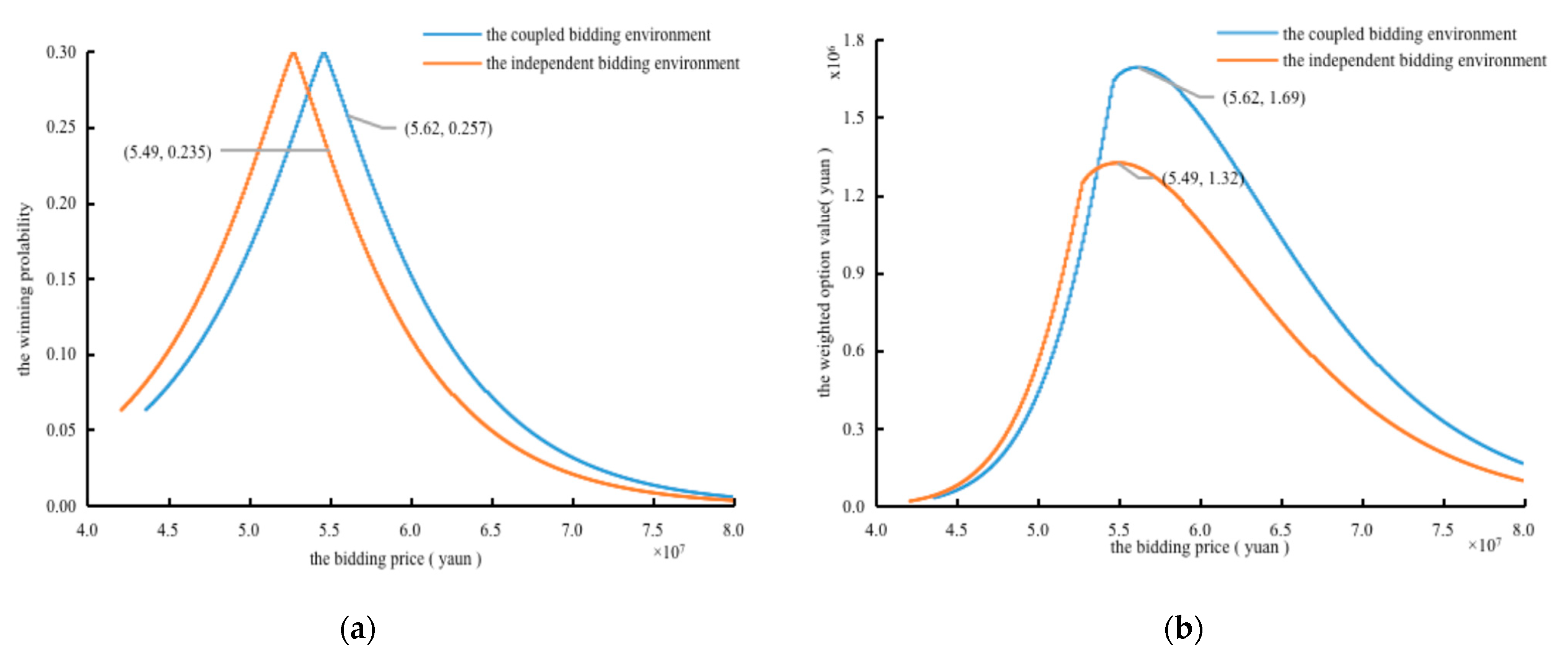
The external competitive environment can be assumed to be the independent and the coupled bidding environment. The independent bidding environment refers to the application of this research method only by the bidding enterprises themselves, and the coupled bidding environment means that the external environment all adopts the independent bidding price method.
(3)
The historical bid-winning data of the external competitive environment is publicly available.
(4)
In the group-independent bidding environment, the individual price decisions in the external competitive environment are independent of each other, and the group price follows the random distribution. In the group coupling bidding environment, it is believed that individual price guesses the group price outside itself and determines its optimal price through group price coupling.
(5)
The competition environment is equitable, and there are no behaviors that violate the law or morality such as vicious competition.

2.2. The Option Value Calculation

Set P as the price made by the bidder and remain unchanged; t as a moment in the bidding preparation stage; Ct as estimated construction costs for the bidder in the bidding preparation stage. In the option period, the construction costs are an uncertain factor. According to the Black–Scholes option pricing model, the estimated construction cost Ct follows the geometric Brownian motion.
d C t = μ C t d t + σ C t d N t
where dCt is the change of estimated costs within dt time interval; μ is the drift percentage; σ is estimated costs volatility; Nt is a Wiener process, also known as Brown motion; dNt is the increments of the standard Wiener process; μ and σ are constants, usually based on the past bidding data, to represent the expected future investment costs trends.
Assuming that the moment when the bidder is selected and invited to sign the contract is T, the bidder’s profit at T is:
max ( [ ( P C T ) ; 0 ] )
If the expected construction costs are higher than the bidding price in the bidding document at T, the winning bidder can choose not to sign the contract. Only when the expected profit is positive at T, the winning bidder will choose to sign. Since the bidding price, P, is fixed when the bidder submits the bidding documents, and the estimated cost, Ct, is flexible during the project execution period, the option income at T is similar to that of the put option. The put option means that if the market price of the underlying future asset falls below the exercise price (bidding price), P, the holders (the winning bidder) can make a profit by taking the initial price (price higher than the current market price), P, as the final exercise price.
The put option formula in the Black–Scholes model is as follows:
P ( S t ,   X ) = X e r ( T t ) N ( d 2 ) S t N ( d 1 )
d 2 = l n S t X ( r 1 2 σ 2 ) ( T t ) σ T t = l n S t X ( r 1 2 σ 2 ) T σ T
d 1 = d 2 σ T
where P′ is the put option value; St is the current price of the asset being traded; X is the option delivery price; r is the risk-free interest rate; T′ is the option period, with year as the unit; N(·) is the cumulative probability distribution function of a normally distributed variable; σ2 is the annualized variance.
In the field of construction project, P≡X, Ct≡St. The option value F of the contract signed at any time when t < T can be expressed as:
F ( P ,   C t ) = P e r ( T t ) N ( d 1 ) C t N ( d 2 )
d 1 = ln P C t ( r 1 2 σ 2 ) ( T t ) σ T t
d 2 = d 1 σ T t
where T − t is the option period, that is, the period from making price decisions to winning the final bid, in the unit of the year.

2.3. The Winning Probability and the Weighted Option Value Calculation

2.3.1. The Winning Probability Calculation

To enhance the external environmental impact of the bidding price and to form a universally applicable winning probability prediction model, in this research, the winning probability is correlated with the average group bidding price, which is regarded as the maximum benchmark price of the probability. If the bidding price deviates from the group characteristics, the winning probability will be reduced. The enterprise will predict the number of competitors and their prices by analyzing published bidding data and assuming that independent competitors will continue the same bidding strategy when bidding in groups. At the same time, due to the differences in the characteristics of the bidding projects, the market information asymmetry, the liquidity of market resources and the scientific differentiation of bidding decisions among enterprises, the bidding environment is divided into the independent and the coupled. In an independent environment, it is assumed that each price is not based on other prices, the bidder can deduce each competitor’s price separately and calculate their maximum value and optimal price jointly. Additionally, in the coupled environment, it is assumed that each competitor also improves its winning probability by predicting others in the group and incorporating its decision basis. The average is taken as the arithmetic mean, and the ratio of the sum of the group bidding price to the total number of bidders is taken. The winning probability formula of the ith (i = 1,2, …, N) competitor is as follows:
W i ( P i ,   C i ) = u × e b ( | P i A P i | A P i ) n
A P i = i = 1 N P i N
where the Ci and Wi are the estimated cost and winning probability of the ith competitor, respectively. N is the number of competitors; Pi is the bidding price of the i-th competitor; the APi is the average group bidding price of the ith competitor; n, b and u are the constant calibration parameters, connection the bidding price and the winning probability; and u represents the winning probability when the APi is equal to the Pi.

2.3.2. The Weighted Option Value Calculation

The winning probability and the maximization of option value are the dual objectives pursued by the enterprise. In this model, the double objectives are transformed into single objectives by multiplication as a decision function, as shown in Equations (11)~(13).
V i ( P i ,   C i ) = F i ( P i ,   C i ) W ( P i ,   C i )
                                                                                V i ( P i ,   C i ) = m a x { [ P i e r ( T t ) N ( d 1 i ) C i N ( d 2 i ) ] [ u × e b ( | P i A P i | A P i ) n ] }
{ [ P i e r ( T t ) N ( d 1 i ) u e b ( A P i P i A P i ) n ] + [ P i e r ( T t ) N ( d 1 i ) C i N ( d 2 i ) ] [ u b n e b ( A P i P i A P i ) n ( A P i P i A P i ) n 1 1 A P i ] = 0 ,           P i < A P i [ P i e r ( T t ) N ( d 1 i ) u e b ( P i A P i A P i ) n ] + [ P i e r ( T t ) N ( d 1 i ) C i N ( d 2 i ) ] [ u b n e b ( P i A P i A P i ) n ( P i A P i A P i ) n 1 1 A P i ] = 0 ,           P i A P i
where the Vi is the option value weighted by the winning probability of the ith competitor. In an independent environment within a group, the prices of each competitor is not affected by other bidding decisions, that is, the Pi follows the random distribution in [Ci,PM], where PM is the bidding control price, and AP1 = AP2 = … = APN.
The bidder divides the competitive environment according to the actual situation and matches the estimated bids of competitors with the bidding environment through the above model. Finally, the bidder replaces itself into the decision-making body of the model and makes comprehensive decisions according to Formula (9)~(13), to enhance the scientific price and improve the winning probability.

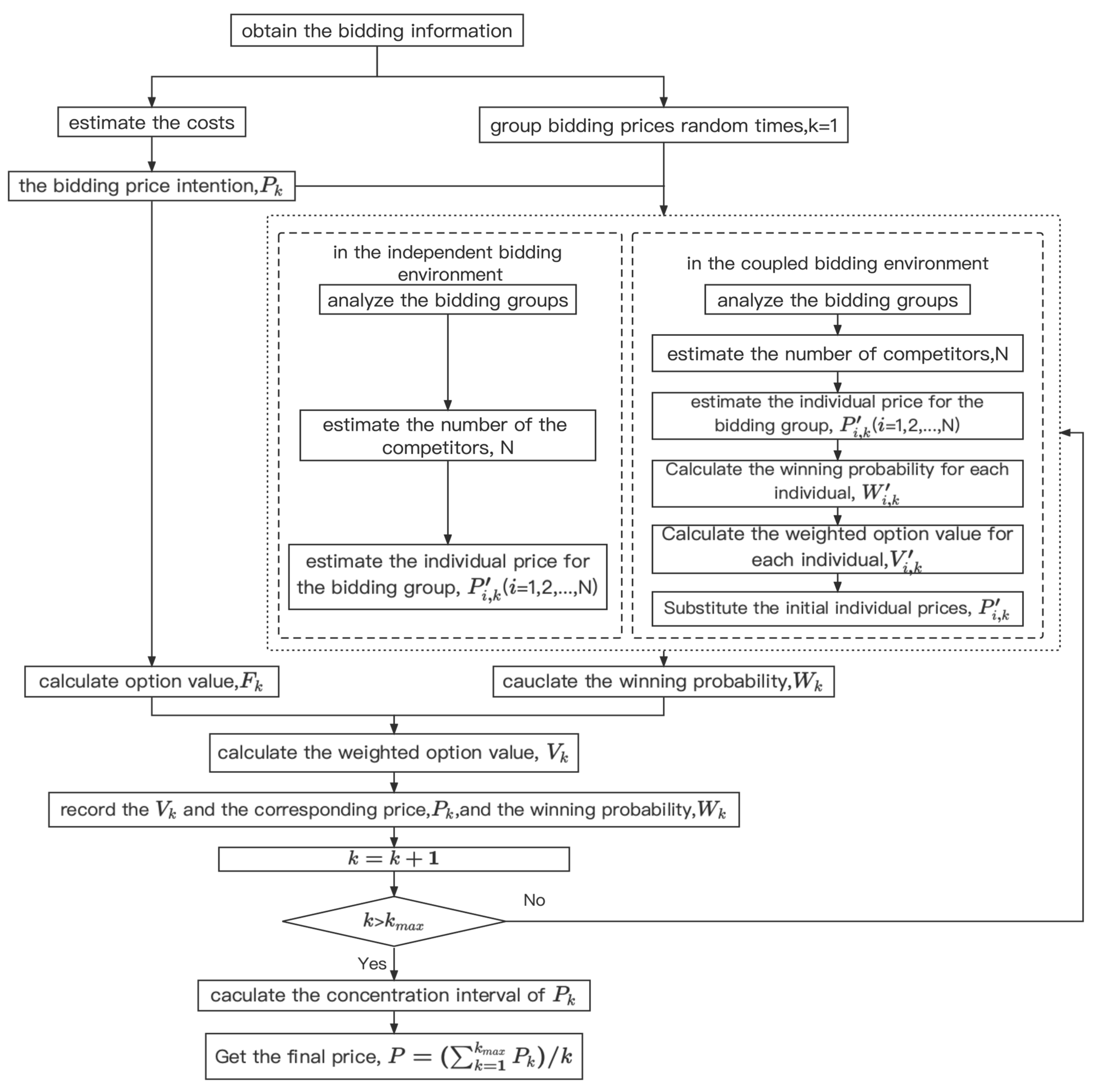
2.4. The Model Framework

Based on the above basic theory of real option pricing, a real option pricing model for construction projects under the group bidding environments is constructed. The model framework is shown in Figure 1. By analyzing the characteristics of the project information, the enterprise sorts out the bidding direction and development prospects of the enterprise in the bidding project under the group bidding environments. Based on the real option pricing theory, according to the market survey data, identify the characteristics of the bidding environment, estimate the costs, the number of competitors, the bidding price of each competitor and other parameters. The option value and the winning probability are calculated to get the weighted option value and the corresponding bidding price. At the same time, to control the influence of uncontrollable and unknown bidding prices of group competitors on the predicted results, the bidding environment is randomly generated several times to obtain the optimal concentration interval, and the average is taken as the final decision.

3. The Model Application and Analysis

3.1. Example Background

Suppose an enterprise conducts in-depth research on a project according to the bidding documents given by the owner and analyzes the published data in the group bidding environments. The enterprise finally determines the value of model parameters, as shown in Table 1. At the same time, a random function was used to observe the bidding situation of competitors. The bidding prices of competitors ranged from CNY 45 million to CNY 60 million, with an average value of CNY 52.79 million. The bidding price of the i-th competitor.

3.2. Simulation Results Analysis in the Independent Bidding Environment

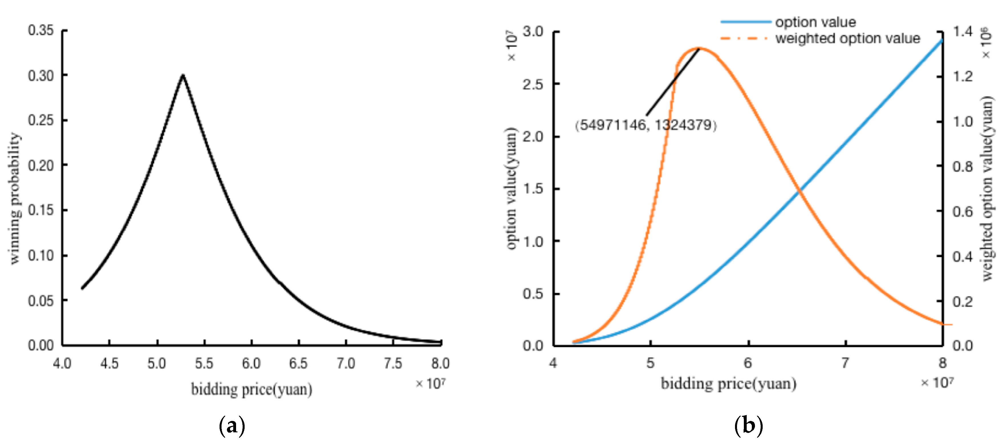
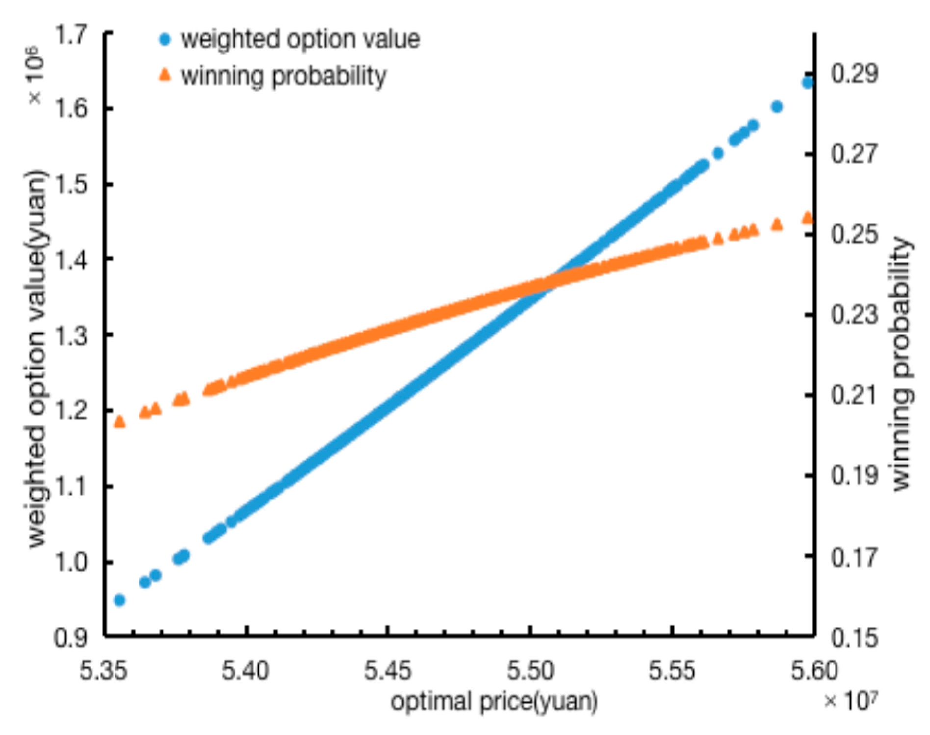
3.2.1. The Optimal Bidding Price Analysis

The changing trend of the winning probability and the option value before and after weighted by the winning probability is obtained, as shown in Figure 2.
When other conditions remain fixed, the option value increases continuously with the higher bidding prices. In other words, without considering the impact of bidding prices on the winning probability, the enterprise will obtain greater benefits with the higher bidding price. However, in the group bidding environments, the option value must be weighted by the winning probability.
The winning probability increases first and then decreases due to the deviation degree of the price and the group characteristics. Therefore, the option value weighted by the winning probability has the maximum objective function and the optimal bidding price. The optimal numerical solution of the model is 5.50 × 10⁷ CNY, which is 0.15% higher than the analytical solution, mainly affected by the iteration step size. It is considered that the numerical solution is consistent with the analytical solution, and the numerical solution model can be used for correlation analysis.
The random competitive prices environment was selected 1000 times to obtain the distribution of the optimal prices group, as shown in Figure 3. It can be seen that the P* is mainly concentrated in the range of CNY [5.41 × 10⁷, 5.54 × 10⁷], with a concentration of 95%. The pricing interval is about CNY 1.3 million, accounting for 2.6% of the costs, which has reduced the pricing range effectively. The average value of the pricing range is taken as the final bidding price, that is, (P*, V) = (54,734,934, 1,251,837).

3.2.2. The Sensitivity Analysis of Parameters

(1)
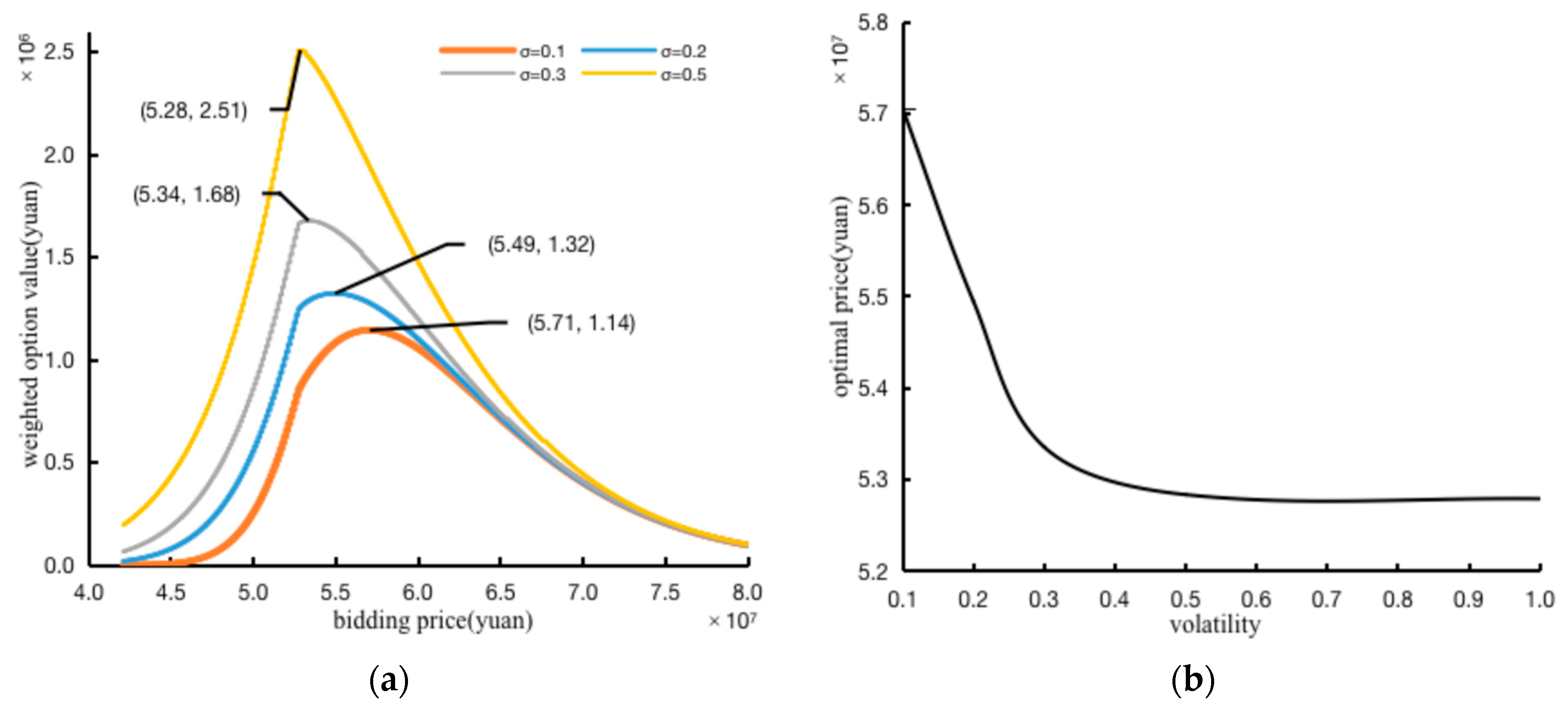
Sensitivity analysis of the volatility level
The estimated costs in the bidding preparation stage have volatility, due to the changes in market environments. The one-way sensitivity analysis of the cost volatility level, σ, is carried out, and the results are shown in Figure 4. With the increase in the volatility level, the maximum weighted option value increases, while the price corresponding to it, the optimal price, decreases. In other words, with the increase in the uncertainty of the market environments, the competitors will put forward a lower bidding price to obtain a higher option value, thus the average value of group bidding prices will be reduced. Then, the enterprise will put forward a bidding price closer to the average, to obtain a greater option value.
To study the relationship between the optimal price and the volatility level further, the curve is shown in Figure 4b. As the volatility decreases, the sensitivity of the optimal price increases, and when the volatility is less than 25%, the optimal price changes nearly linearly, then it decreases gently until the volatility exceeds 40%, and the curve tends to be stable. This is because the enterprise will only lower the bidding price for a higher probability under the condition of ensuring profits. The optimal bidding price has an average sensitivity of 9.77% to the volatility.
Therefore, the results of the one-way sensitivity analysis of the cost volatility level indicate that in the actual bidding process, the market environment should be estimated in the bid preparation stage to sort out the factors that may have an impact on the costs and the scope of it after the price decision, especially in the construction stage of the project. If the market environment is more volatile, a higher option value can be obtained by lowering the bidding price to reduce the degree of group deviation. At the same time, the timing of the estimated costs decision can be postponed to reduce the impact of uncertainty in the market environment on the bidding price decision.
(2)
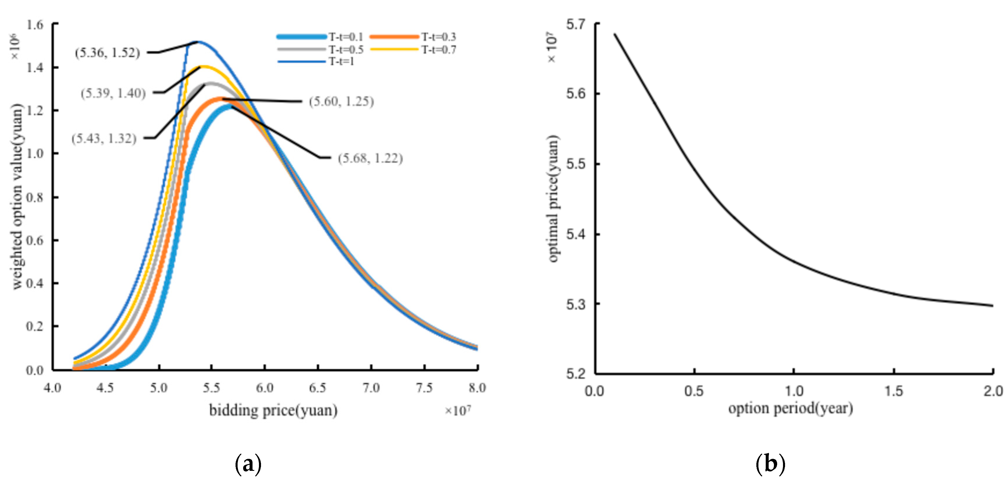
The Sensitivity Analysis of The Option Period
The one-way sensitivity analysis of the option period, T – t, is carried out, and the results are shown in Figure 5. With the extension of the option period, the maximum weighted option value increases, while the optimal price decreases. In other words, with the extension of the period from the determination of the bidding price to the final winning, the uncertainties of the internal and external environments faced by the enterpriser will increase, and the competitors will propose lower prices to increase the winning probability, thus the average value of group bidding prices will be reduced. Then, the enterprise will put forward a price closer to the average, to obtain a greater option value.
To study the relationship between the optimal price and the option period further, the curve is drawn as shown in Figure 5b. As the extension of the period, the sensitivity of the optimal price decreases, and when the period is less than 0.5 years, the optimal price makes a linear response to the option period. That is because if the period is short, the enterprise will pay more attention to the influence of internal strength which tends to be stable in a short time. Then, it decreases gently until the period exceeds 1.5 years, and the curve tends to be stable. The optimal bidding price has an average sensitivity of 7.70% to the period.
Thus, the results of the one-way sensitivity analysis of the option period indicate that in the actual bidding process, it is necessary for companies to anticipate the length of the option period in the bidding preparation stage. Additionally, it is necessary to use a real option pricing model to anticipate the trend of the volatility of the optimal price over a certain range of option expiration dates. Take this project as an example: if the option period is expected to be within 0.5 years, the bidding price can be increased within a reasonable range according to the real option pricing model of group bidding. If the option period is expected to be more than 1.5 years, to improve the winning probability, the bidding price can be reduced to control the degree of group deviation.
(3)
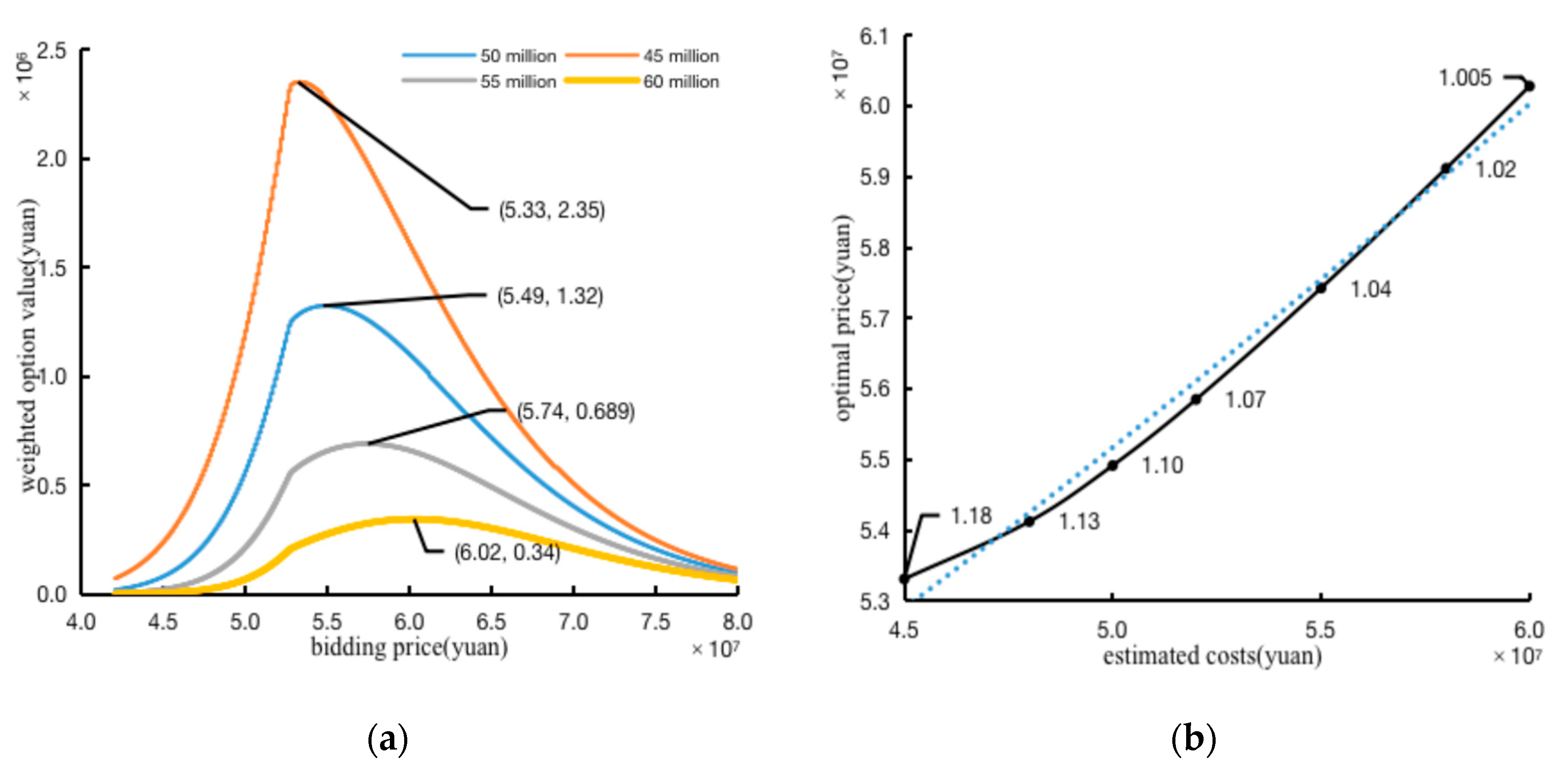
The Sensitivity Analysis of The Estimated Costs
As an important factor in price decision making, the estimated costs in the bidding preparation stage are different during the same period of different enterprises or different periods of the same enterprise. The one-way sensitivity analysis of the estimated costs, Ct, is carried out, and the results are shown in Figure 6. With the increase in the estimated costs, the maximum weighted option value shows a downward trend, and the optimal price shows an upward trend. This is because considering the pricing strategy in the group bidding environments, with the increase in the estimated costs of the enterprise, the less space to markup and the lower the winning probability, the lower value.
To study the relationship between the optimal price and the estimated costs further, the curve is drawn as shown in Figure 6b, in which the ratio of optimal price to corresponding estimated costs, in other words, the optimal mark-up ratio, has been marked. As can be seen from the figure, in the same bidding project, as the estimated costs rise, the mark-up space on this basis shrinks, the optimal price is less sensitive to the estimated costs, and the optimal mark-up ratio decreases. If the estimated costs are too high, the optimal price will tend to respond linearly, that is, no matter what the estimated costs are, the optimal mark-up ratio remains the same, with an average mark-up ratio of 1.078 and an average sensitivity of 35.06%.
Therefore, the results of the analysis on estimated cost show that, in the actual bidding process, the enterprises should combine the internal resource environment and external competitive environment, reduce the cost as far as possible, expand the markup space and enhance the sensitivity to the estimated cost. To obtain higher option value and improve the winning probability, at the same time, based on the group bidding pricing model, the optimal markup ratio of the project is estimated according to the decision flexibility.
(4)
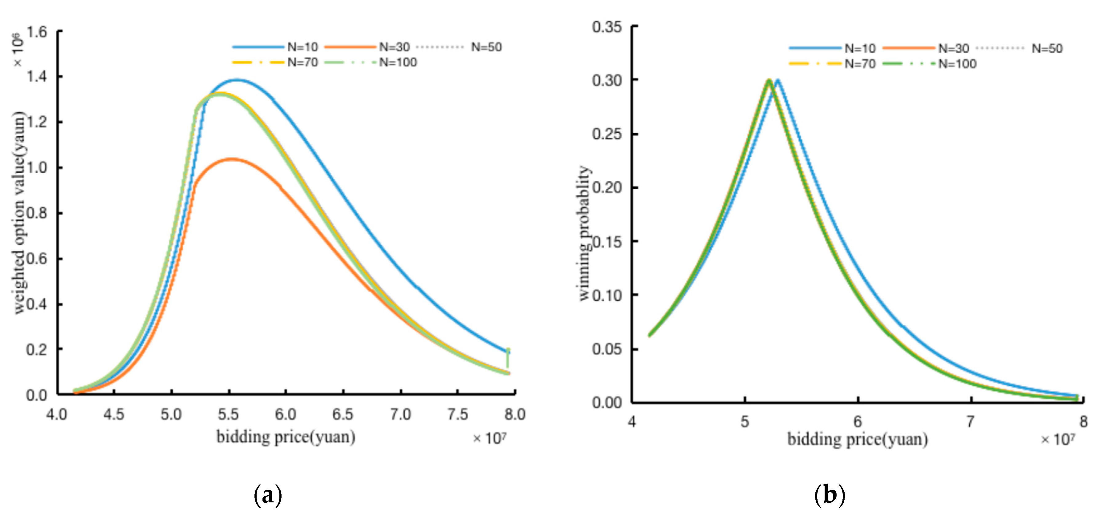
The Sensitivity Analysis of The Number of Competitors
The characteristics of the bidding price data under different numbers of competitors are summarized in Table 2, with the same average value and the similar maximum, minimum and median values.
The one-way sensitivity analysis of the number of competitors, N, is carried out, and the results are shown in Figure 7. The bidding price, weighted option value and the winning probability are not sensitive to changes in the number of competitors in the same bidding project. This is because the bidding price is more influenced by the average than the number of competitors. Assuming that the other parameters are constant, an increase or decrease in the number of competitors does not affect the trend in the winning probability and the weighted option value when there is no significant change in the average.

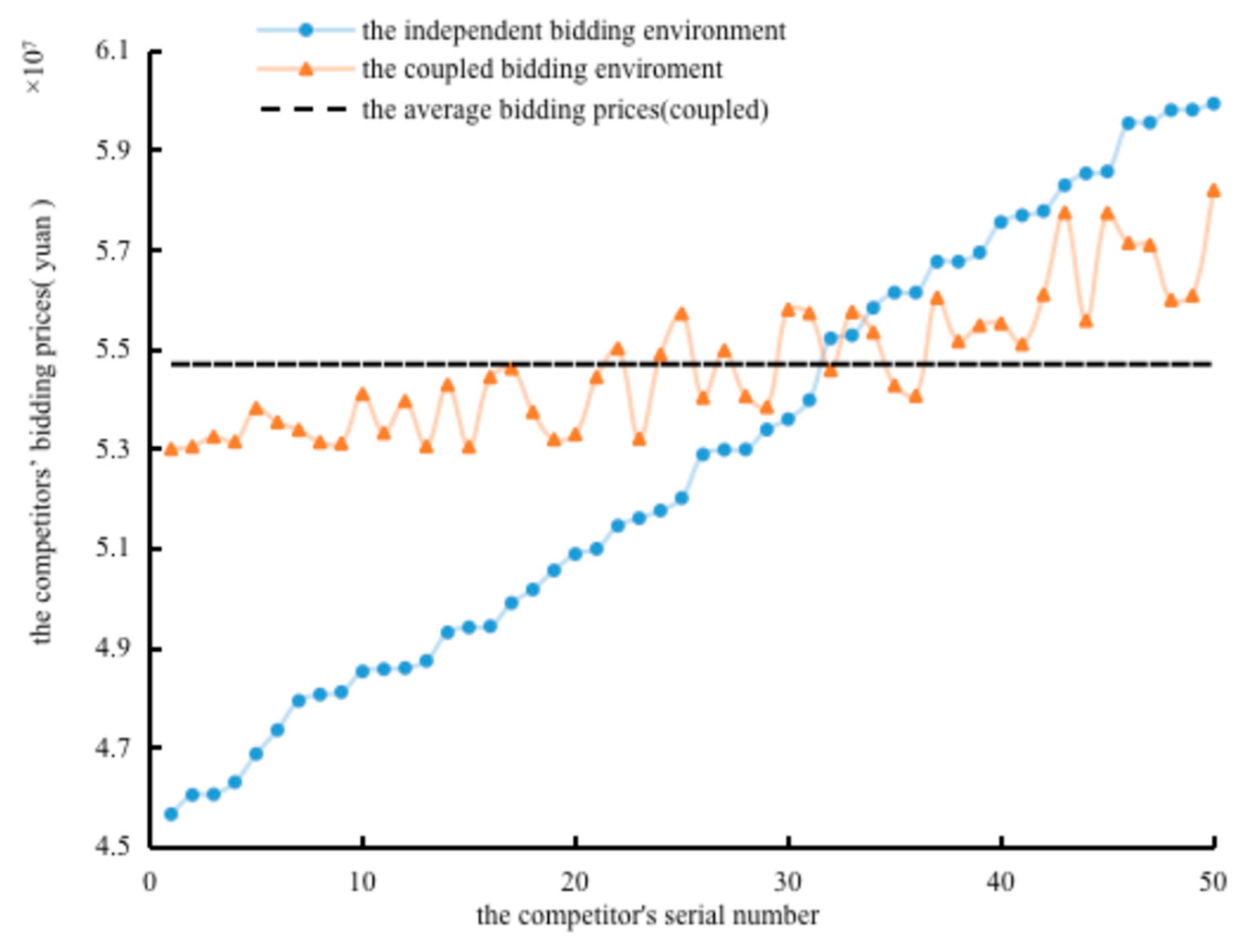
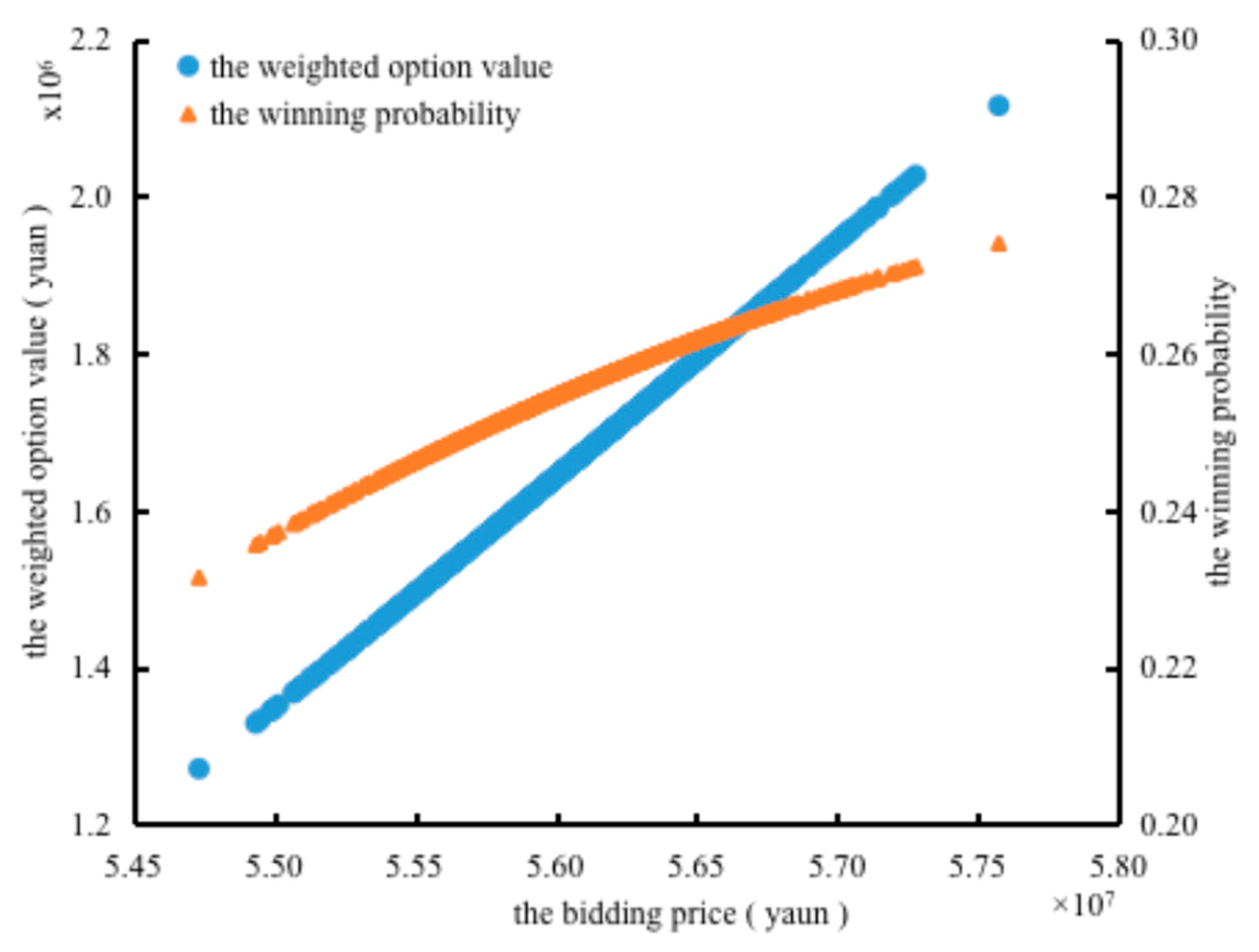
3.3. Simulation Results Analysis in the Coupled Bidding Environment

The bidding prices of competitors in the coupled bidding environment are calculated and compared with the independent bidding environment as shown in Figure 8. The bidding prices optimized by the coupling environment are more concentrated near the average value than the initial price. This is because the competitor I is more inclined to make decisions to reduce the internal deviation value of the group to improve the winning probability by predicting other prices.
Under the coupled bidding environment, the trend of the winning probability and the weighted option value are calculated, and the comparison with the trend in the independent environment is shown in Figure 9. In both bidding environments, as the bidding price increases, the winning probability and the weighted option value both increase first and then decrease. The optimal price in the coupled competitive environment is significantly higher than that in the independent environment. This is because, in the coupled bidding environment, the enterprises can reduce the degree of group deviation by improving the rationality of the group bidding environment prediction, so that the bidding price is closer to the group characteristics. Therefore, the winning probability and the weighted option value by the winning probability also tend to rise, and the bidding price corresponding to the maximum weighted option value, that is, the optimal price, increases accordingly. The optimal price increased by about 2.37%, and the corresponding winning probability and the weighted option value increased by about 9.36% and 28.03%, respectively.
The random competitive prices environment was selected 1000 times to obtain the distribution of the optimal prices group, as shown in Figure 10. It can be seen that the P* is mainly concentrated in the range of CNY [5.51 × 10⁷, 5.72 × 10⁷], with a concentration of 95%. The pricing interval is about CNY 2.1 million, accounting for 4.6% of the costs, which has reduced the pricing range effectively. The average value of the pricing range is taken as the final bidding price, that is, (P*, V) = (54,734,934, 1,251,837). The bidding price comprehensive decision is 2.48% higher than independent competition environment.

4. Conclusions and Prospects

This research provides direct support for bidding price by establishing a real option pricing decision of the construction projects under group bidding environments, and the specific conclusions are as follows:
(1) Based on the real option value theory, the competitive group behavior is divided into the independent and coupled bidding. By analyzing independent random competitive groups, the real option pricing theory is applied to the complete bidding price decision-making process. The analysis shows that the model has certain reliability and validity, improves the objective degree of the bidding decision-making environment and promotes the competitive ability of price decision making.
(2) The changes in the optimal bidding price are proportional to the estimated costs, inversely proportional to the volatility level, option period, and independent of the number of competitors. However, the changes in the weighted option value are inversely proportional to the estimated costs, directly proportional to the cost volatility level and option period, and independent of the number of competitors. The sensitivity of the optimal price to the estimated costs, the costs volatility level and the option period are 35.06%, 9.77% and 7.70%, respectively, and the average optimal mark-up ratio is 1.078. Through the comparison of price decisions under independent and coupled bidding environments, it is found that the price group of competitors in the coupled bidding environment is more concentrated around the average value than the initial, and the optimal price of the enterprises increases significantly. The corresponding winning probability and the weighted option value also showed an upward trend, increasing by about 2.37%, 9.36% and 28.03%, respectively.
(3) The results of the one-way sensitivity analysis of each parameter indicate that in the actual bidding process, the estimated costs and the option period should be estimated in the preparation stage. To improve the winning probability and obtain the higher option value, rely on the estimated fluctuation of the optimal bidding prices within a certain option period, increase the bidding price within a reasonable range when the market environment is more stable and lower the price to reduce the group deviation degree when the degree of uncertainty in the market environment is high, while postponing the timing of the estimated cost decision. At the same time, the cost is reduced as much as possible, the bidding price markup space is expanded, the sensitivity to the estimated costs is enhanced and the optimal markup ratio of the project is estimated according to the flexibility of decision making based on the group bidding pricing model.
This research assumes that in a group bidding environment, an enterprise obtains its maximum value and optimal price decision by inferring bidding prices of independent or coupled competitors separately and jointly calculating. The results can be used in the bidding price decision, through the optimization of the price, to improve the winning probability. The model is applicable to project bidding with option concept, but some environmental parameters need to be optimized according to the characteristics of the industry and bidding group. In the actual bidding project, due to the limited construction engineering market resources, accurate prediction of the correlation level among the competitors is the premise of making a reasonable bidding decision. Future research should consider distinguishing bidding price coupling degrees among different competitors in the coupled bidding environment, to optimize the comprehensive price decision. At the same time, all parameters jointly determine the decision of joint restriction price. In the future, the coupling degree between parameters should be considered to explore the comprehensive decision under the influence of multiple factors.

Author Contributions

Methodology, M.L. and C.Z.; supervision, M.L.; writing—original draft, C.Z.; writing—review and editing, M.L. All authors have read and agreed to the published version of the manuscript.

Funding

This research received no external funding.

Institutional Review Board Statement

Not applicable.

Informed Consent Statement

Not applicable.

Data Availability Statement

Some or all data, models or code that support the findings of this study are available from the corresponding author upon reasonable request.

Conflicts of Interest

There is no conflict of interest regarding the publication of this paper.

References

  1. Kagel, J.H.; Levin, D. Common Value Auctions and the Winner’s Curse; Princeton University Press: Princeton, NJ, USA, 2002. [Google Scholar] [CrossRef] [Green Version]
  2. Lei, M.; Yin, Z.H.; Deng, S.J.; Wei, Y.N.; Qian, W.; Li, Z. Why is below average bid auction preferred in procurement? South China J. Econ. 2018, 37, 61–84. [Google Scholar]
  3. Ioannou, P.G.; Leu, S.S. Average-bid method—Competitive bidding strategy. J. Constr. Eng. Manag. 1993, 119, 131–147. [Google Scholar] [CrossRef] [Green Version]
  4. Zheng, X.T. Equilibrium Bidding Behaviors and Collusion Incentives in BAMs. South China J. Econ. 2010, 246, 46–62. [Google Scholar]
  5. Zheng, X.T.; Zhang, Y.G.; Lu, Y.F. An Experimental Study on Average-price-win Auction: The Tradeoff between Avoiding Winner’s Curse and Cutting Price. Ind. Econ. Rev. 2011, 12, 52–63. [Google Scholar]
  6. Friedman, L.A. Competitive-bidding strategy. Oper. Res. 1956, 4, 104–112. [Google Scholar] [CrossRef]
  7. Davatgaran, V.; Saniei, M.; Mortazavi, S.S. Optimal bidding strategy for an energy hub in energy market. Energy 2018, 148, 482–493. [Google Scholar] [CrossRef]
  8. Rastegar, H.; Arbab, S.B.; Mirmohammadi, S.H.; Bajegani, E.A. Stochastic programming model for bidding price decision in construction projects. J. Constr. Eng. Manag. 2021, 147. [Google Scholar] [CrossRef]
  9. Takano, Y.; Ishii, N.; Muraki, M. A sequential competitive bidding strategy considering inaccurate cost estimates. Omega 2014, 42, 132–140. [Google Scholar] [CrossRef]
  10. Zou, X.H. Research on the Application of the Maneuver Tree of Tendering and Bidding. Commer. Res. 2002, 8, 84–85. [Google Scholar]
  11. Christodoulou, S. Bid mark-up selection using artificial neural networks and an entropy metric. Eng. Constr. Archit. Manag. 2010, 17, 424–439. [Google Scholar] [CrossRef]
  12. Hosny, O.; Elhakeem, A. Simulating the winning bid: A generalized approach for optimum markup estimation. Autom. Constr. 2012, 22, 357–367. [Google Scholar] [CrossRef]
  13. Hao, L.P.; Tan, Q.M.; Ge, Y. Study on Strategies Making of Project Offering Based on Game Model and Fuzzy Forecasting. J. Ind. Eng. Eng. Manag. 2002, 16, 94–96. [Google Scholar]
  14. Chen, J.; Fu, H.Y. Research on evolution game of multi-stakeholder collusion in project bidding. J. Railw. Sci. Eng. 2019, 16, 2378–2386. [Google Scholar] [CrossRef]
  15. Assaad, R.; Ahmed, M.O.; El-Adaway, I.H.; Elsayegh, A.; Nadendla, V.S.S. Comparing the Impact of Learning in Bidding Decision-Making Processes Using Algorithmic Game Theory. J. Manag. Eng. 2020, 37, 04020099. [Google Scholar] [CrossRef]
  16. Jiang, G.P.; Wang, W.D.; An, J. Optimal Price Decision of Bidding Based on Prospect Theory. J. Wuhan Univ. Technol. Inf. Manag. Eng. 2012, 34, 353–356. [Google Scholar]
  17. You, T.H.; Cao, B.B. A Method for Bid Price Decision Making Considering Bidder’s Psychological Behaviors and Normal Distribution. J. Eng. Manag. 2017, 31, 19–23. [Google Scholar]
  18. Engelbrecht-Wiggans, R.; Katok, E. Regret and Feedback Information in First-Price Sealed-Bid Auctions. Manag. Sci. 2008, 54, 808–819. [Google Scholar] [CrossRef] [Green Version]
  19. Chen, Z.D.; Zou, Q.L. Risk Analysis and Evaluation of Hydropower EPC Project Cost Based on Entropy Weight. Water Resour. Power 2015, 33, 168–171. [Google Scholar]
  20. Li, J.Q.; Zhan, W.J.; Zhang, J.L.; Wang, S.Y. Methods for Bidding under Risk. Oper. Res. Manag. Sci. 2002, 11, 1–10. [Google Scholar]
  21. Biancardi, M.; Bufalo, M.; Di Bari, A.; Villani, G. Flexibility to switch project size: A real option application for photovoltaic investment valuation. Commun. Nonlinear Sci. Numer. Simul. 2023, 116, 106869. [Google Scholar] [CrossRef]
  22. Zhang, M.M.; Zhou, P.; Zhou, D.Q. A real options model for renewable energy investment with application to solar photovoltaic power generation in China. Energy Econ. 2016, 59, 213–226. [Google Scholar] [CrossRef]
  23. Yang, W.; Fang, N.; Wang, Y.; Long, T.; Deng, S.; Xue, M.; Deng, B. Value evaluation of mining right based on fuzzy real options. Resour. Policy 2022, 78, 102818. [Google Scholar] [CrossRef]
  24. Zhang, H.; Assereto, M. Deferring real options with solar renewable energy certificates. Glob. Financ. J. 2022, 55, 100795. [Google Scholar] [CrossRef]
  25. Yang, A.; Meng, X.; He, H.; Wang, L.; Gao, J. Towards Optimized ARMGs’ Low-Carbon Transition Investment Decision Based on Real Options. Energies 2022, 15, 5153. [Google Scholar] [CrossRef]
  26. Black, F.; Scholes, M. The pricing of options and corporate libilities. J. Political Econ. 1973, 81, 637–654. [Google Scholar] [CrossRef]
Figure 1. The real option pricing decision framework.
Applsci 13 01130 g001
Figure 2. Optimal decision determination of bidding price. (a) Fluctuation trend of winning probability; (b) Fluctuation trend of option value and weighted option value.
Applsci 13 01130 g002
Figure 3. Concentration of the optimal bidding price.
Applsci 13 01130 g003
Figure 4. Sensitivity analysis of volatility. (a) Volatility sensitivity; (b) Fluctuation trend of optimal price. (Ct = 50,000,000; b = 10; n = 1.1; u = 0.3; r = 0.01; T-t = 0.5; N = 50; APcomps = 52.79 million).
Applsci 13 01130 g004
Figure 5. Sensitivity analysis of the option period. (a) Period sensitivity; (b) Fluctuation trend of optimal price. (Ct = 50,000,000; b = 10; n = 1.1; u = 0.3; r = 0.01; σ = 0.2; N = 50; APcomps = 52.79 million).
Applsci 13 01130 g005
Figure 6. Sensitivity analysis of the estimated costs. (a) Costs sensitivity; (b) Fluctuation trend of optimal price. (b = 10; n = 1.1; u = 0.3; r = 0.01; σ = 0.2; T-t = 0.5; N = 50; APcomps = 52.79 million).
Applsci 13 01130 g006
Figure 7. Sensitivity analysis of the number of competitors. (a) Numbers sensitivity; (b) Numbers sensitivity. (Ct = 50,000,000; b =10; n = 1.1; u = 0.3; r = 0.01; σ = 0.2; T-t = 0.5; APcomps = 52.79 million).
Applsci 13 01130 g007
Figure 8. The bidding prices of competitors in independent and coupled bidding environments.
Applsci 13 01130 g008
Figure 9. The optimal price decision comparison. (a) Fluctuation trend of the winning probability; (b) Fluctuation trend of the weighted option value.
Applsci 13 01130 g009
Figure 10. The concentration of the optimal bidding price.
Applsci 13 01130 g010
Table 1. The Value and meaning of parameters.
ParameterValueMeaning
CtCNY 50 millionestimated investment costs
σ20%estimated costs volatility level
r1%risk-free rate of return
T − t0.5 yearsThe option period
n1.1calibration parameter
b10calibration parameter
u0.3calibration parameter
N50Number of competitors
Pi-the bidding price of the i-th competitor
Table 2. The bidding prices of competitors.
Prices (CNY Ten Million)AverageMaximumMinimumMedian
Numbers
105.2795.6934.8065.291
305.2795.8424.7105.231
505.2795.9924.5645.243
705.2795.8564.6865.292
1005.2795.9924.5645.243
Disclaimer/Publisher’s Note: The statements, opinions and data contained in all publications are solely those of the individual author(s) and contributor(s) and not of MDPI and/or the editor(s). MDPI and/or the editor(s) disclaim responsibility for any injury to people or property resulting from any ideas, methods, instructions or products referred to in the content.

