Prediction of Emotional Empathy in Intelligent Agents to Facilitate Precise Social Interaction

Abstract

The research area falls under the umbrella of affective computing and seeks to introduce intelligent agents by simulating emotions artificially and encouraging empathetic behavior in them, to foster emotional empathy in intelligent agents with the overarching objective of improving their autonomy. Raising the emotional empathy of intelligent agents to boost their autonomic behavior can increase their independence and adaptability in a socially dynamic context. As emotional intelligence is a subset of social intelligence, it is essential for successful social interaction and relationships. The purpose of this research is to develop an embedded method for analyzing empathic behavior in a socially dynamic situation. A model is proposed for inducing emotional intelligence through a deep learning technique, employing multimodal emotional cues, and triggering appropriate empathetic responses as output. There are 18 categories of emotional behavior, and each one is strongly influenced by multimodal cues such as voice, facial, and other sensory inputs. Due to the changing social context, it is difficult to classify emotional behavior and make predictions based on modest changes in multimodal cues. Robust approaches must be used to be sensitive to these minor changes. Because a one-dimensional convolutional neural network takes advantage of feature localization to minimize the parameters, it is more efficient in this exploration. The study’s findings indicate that the proposed method outperforms other popular ML approaches with a maximum accuracy level of 98.98 percent when compared to currently used methods.

1. Introduction

Artificial Intelligence (AI) is computer science’s most empowering and optimistic branch. Simulated intelligence, which aspires to be one step ahead, focuses on the most perplexing, complex, cumbersome, and exhausting problems that cannot be easily comprehended using conventional algorithmic methods [1]. It cannot obtain proper recognition in a single domain, which is misleading. Doyle’s definition of AI is as follows: “It is the science of comprehending intelligent creatures through the development of Intelligent Agents (IA) that are currently affecting the entire world and its living standards.” With significant advancements in AI and other mechanical domains, IAs are becoming increasingly coordinated across societal regions. IAs are multifunctional models that can be reprogrammed/customized [2,3].

Empathy has a sordid history, marked by disagreement and inconsistency. Although it has been researched for millennia, with significant contributions from philosophy, theology, experimental psychology, individual and social psychology, ethology, and neuroscience, the field struggles with a lack of agreement concerning the phenomenon’s nature. Despite this difference of opinion, empirical evidence for empathy is completely compatible across various species [4]. The act of understanding another person’s emotions and sharing their emotional experiences is known as Emotional Empathy (EE). This profound awareness of another person’s emotional state usually results from shared experiences [5]. Increasing EE to improve their instinctive behavior can enhance the independence and adaptability of IAs in a socially dynamic setting.

Affective Computing (AC) is perhaps the most recent unit of computer science, having emerged with Rosalind Picard’s paper [6,7]. It is a rapidly growing interdisciplinary field that combines analysts, researchers, and experts from various fields, including psychology, sociology, artificial intelligence, natural language processing, and deep learning [8,9]. However, it does not appear easy to imagine how humans can work seamlessly with machines and IAs. 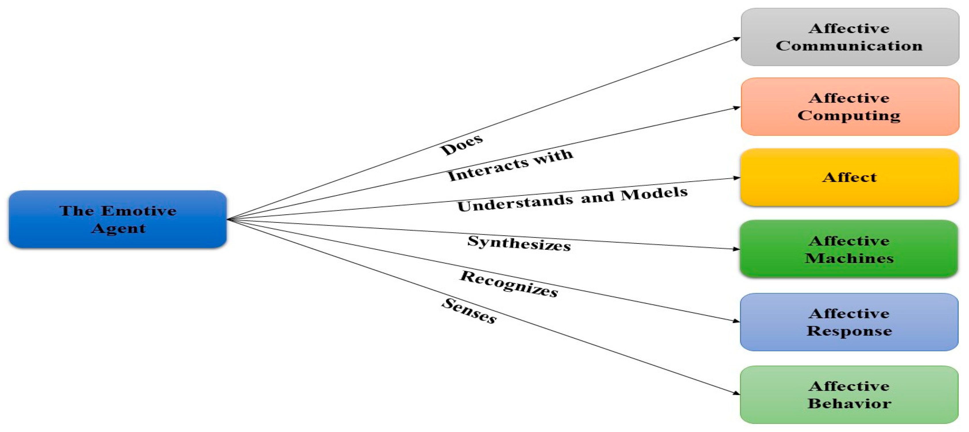AC enables IAs to process data gathered from various sensors to assess an individual’s emotional state, ranging from unimodal analysis to increasingly complex forms of multimodal research [10]. Emotional intelligence (EI) is perplexing from a human perspective, and there is no exact rational explanation or theory. The critical foundation for AC is understanding emotions and their role in human behavior and cognitive processes [11,12]. In the development of AC-based frameworks, pattern recognition and examination techniques are used to recognize and synthesize facial patterns and generate an Emotional Response (ER). It encompasses various facets as shown in Figure 1 [8,13,14].

All three of synthesis, evocation, and regulation contain cognitive and non-cognitive components. The associated ER evokes empathy. It is the capacity to recognize and differentiate among varied social contexts employing cognition and emotions and to respond properly to the associated emotional state. The human brain accommodates multimodal cognitive modeling information as shown in Figure 2.

AC has been made possible by AI-enabled systems due to their rule-based architecture and ability to operate in an interactive and dynamic environment [15,16,17]. The following section focuses on developing Social Interaction (SI) by invoking EE in IAs. SI is an individual’s ability to react appropriately according to the perceived situation from the surroundings for productive social interaction. On the off chance that we want an IA to be a primary essential instrument or a gadget, as a partner, a colleague, and a social helper, it is required to implant SI in those frameworks. In order to support human activities, human beings are social delegates, and IAs should show enough SI to communicate with humans adaptively. If they lacked SI, they would not acquire a secure position in social contexts despite their extraordinary ability.

The IAs would not help humans appropriately if they ignore the weaknesses, lacks, desires, and necessities of humans. In any situation, the sensitive and adaptable response of IAs to the emotions and sentiments of others reflects EE (fundamentally needed to be a functioning social being, as presented in Figure 3) in these frameworks. In order to achieve this, it necessitates the endowment of intellectual capacities in IAs with EI that raise the SI and have empathetic Human-to-Robot Interaction (HRI) or Robot-to-Robot Interaction (RRI) [16,18,19,20,21].

Even though IAs engage in SI, going beyond these boundaries requires a high level of expertise. EE aids in developing various SI-based attributes within these frameworks and enhancing their capabilities and, as a result, the degree of social acceptance. Generally, various human cognitive capacities and abilities are integrated into EI. Except when EI is incorporated into IAs, it is impossible for these systems to respond innovatively, creatively, imaginatively, psychologically, or rationally in social settings. A meaningful and emotive response is required for a friendly personality to emerge [22]. To accomplish this goal, an IAs must exhibit Empathetic Behavior (EB). Certain researchers focus on facial emotion detection, speech emotion detection, cognitive modeling, and other related areas, but prior research has lacked EB detection based on Multimodal Emotional Cues (MECs). However, this research establishes an EB prediction system based on MECs in order to increase the degree of HRI or RRI. As such, this research takes facial and vocal emotional cues and other identified parameters (as input parameters) into account and predicts relevant EB.

We employ a powerful method that has become popular in the literature to handle this massive amount of multimodal data in terms of parameters and occurrences [22]. The other strategies, such as user experience and human–computer interaction, are also well discussed in recent studies highlighting their significance in academia and business [23,24]. Convolutional Neural Networks (CNN) are multi-layer artificial neural networks that outperform traditional approaches in tasks like pattern recognition. The following are the main points of the method: high accuracy and performance when compared to other recognition algorithms on the same dataset in an end-to-end architecture. A CNN is utilized to recognize EB. There is no need for any pre-processing steps. After getting a minimum number of frames, the classification process begins. After new raw input samples, the EB class is predicted almost real-time (sensor data) [25].

Furthermore, we evaluated a method for recognizing emotions from multimodal data, tested on a dataset gathered from various sources. Multimodal emotional cues are used in a social context to identify IA’s emotional behavior. Independent prediction models are used to combine these modalities. In addition, we developed a complete evaluation method to compare impacts on the same dataset under specified and well-defined settings in order to guarantee consistency in various situations and adaptation to real-world conditions. Cross-validation, on the one hand, enables the evaluator to demonstrate the statistical significance of several models, as opposed to depending on the chance that the system works well for one or two cases. On the other hand, the system enables us to analyze its performance in real-world contexts, such as when it is difficult to obtain annotated data from a new user, and the system must rely on information acquired from learning in similar contexts. We examined Machine Learning (ML) and Deep Learning (DL) techniques for dealing with data obtained from multimodal cues, leveraging embeddings from pre-trained deep neural networks, and fine-tuning these models to fit our dataset for categorization and later prediction of EB. During a SI, the representation of emotions undergoes an intensity transition that traverses numerous phases, posing a significant learning challenge for non-temporal models. To the best of our knowledge, just few published data combine MECs with the other EB-influencing parameters described in this work.

1.1. Problem Statement

Human intelligence is an amalgamation of logical reasoning and emotional states. Humans are relatively more induced and motivated by emotional states than by rational thinking. Human emotional activation is elicited by internal and external stimuli and is expressed by physiological signs, e.g., expressions, voice tone, energy, pitch, etc. The better the emotional interaction, the better the interpersonal relationship, and the more it will be sociable. Since IAs do not have to endure and tolerate human-like awkwardness, hardness, severity, tediousness, hungriness, torture, and other such problems, they are better replacements and more adaptable in challenging human working fields. However, due to the lack of understanding of human affective states, they only perform what they are instructed and exhibit brutal, insensitive, and unfriendly behavior. A meaningful and dynamic response is essential for exhibiting a friendly personality. Attainment of this goal requires an IAs to possess EB. In prior studies, some studies dealt with facial emotion detection only or speech emotion detection only, and some deal only with cognitive modeling, etc., and lack skills in providing EB detection based on MECs [26,27]. However, this research caters to MECs (as input parameters) and predicts the respective EB.

1.2. Purpose of the Research

One of the primary goals of AC is empathy: the ability to understand and recognize others’ emotional states and respond accordingly. The IA’s sensitized acceptance and adaptive behavior towards the other user’s emotional state results in more productive and delightful interaction. AC directs the computational modeling of EI to achieve genuineness in HRI collaboration. This SI helps IAs securely coexist and be in touch with humans to control the potency of social interaction with humans. Accordingly, this research is intended to provide a model for EB prediction in response to the inputs through MECs. These models help can work in the future to generate EE-based abilities in the modern IAs, which would be pivotal for enhancing emotional adaptiveness and, consequently, increasing their social acceptance level.

2. Literature Review

This section presents a literature review to shed light on various researchers’ efforts to improve EE in IAs. Several studies on ML and DL highlight their applications in several fields; they have proven to be an excellent source of guidance for the proposed idea.

Various researchers’ efforts shed light on managing EE prediction in IAs to precisely cater to SI through diverse, intelligent techniques. Numerous related studies demonstrated the applications experimentally, which served as an excellent guide for developing the proposed concept of EI and EB into IAs in order to increase their degree of interaction. A few models were provided to aid in developing machine consciousness models with varying degrees of control in execution. Furthermore, AC characteristics, such as emotion, etiquette, and personality traits, have not been a primary focus of machine-consciousness-based models. IAs are deficient in these domains and other programming-based applications. The authors of the study [28] reviewed several existing models of machine consciousness and proposed an AC-based model capable of developing human-like mechanical frameworks. Machine consciousness presented an AC-based model intending to incorporate the emotive characteristics that give AI systems a human-like skill. It is critical for the establishment of AC-based IAs in order to facilitate HRI.

Another study proposed various methods to improve HRI, including emotional affordances. Those are methods that take emotions into account to capture and transmit emotional signals in any situation; they may help to consolidate physical interaction and social norms. For example, with this rich thought, they uncovered the optimal strategy for dealing with EI’s multimodal and unpredictable nature. What are humans’ emotional processes, and how are they related to broader or possibly environmental and social conditions? This effort aimed to develop a framework for the emotional affordances’ structural taxonomy that enables a better understanding of HRI. Along these lines, this research provided an EA-oriented taxonomy to experts in IAs, allowing for the HRI to be upgraded [29].

The identified research presented an AI-based model expected to improve HRI based on the dice game’s situation. It provided an analytical approach based on a case study to address some challenges of this domain: Does an IA with a socially engaging character offer a higher degree of acceptance than a focused one? The presented system possesses the adaptability to create and credit two distinctive qualities to any socially IA possessing a humanoid mien; social engagement attributes increase its degree of interaction and cooperation. A concentrating character focuses on playing and being the game-winner. The two attributes were assessed, and the humans and IAs played the dice game on a turn basis. Throughout the game, each feature was assessed to investigate the members’ emotional facial states. The results indicated that the IA’s interaction was considered better as a friend than a competitor. It was concluded that, in HRI, emotional engagement prompts a high degree of social acceptance [30].

The coordinated effort in HRI settings is receiving continuous importance. Accordingly, there is a growing interest in improving systems that can advance and upgrade the association and collaboration among humans and IAs. One of the pivotal analyses in the HRI field is giving IAs affective and psychological capacities to develop an empathetic relationship with humans. Various models were proposed to meet this challenge. This research provides an outline of the most significant activities through a literature review of the frameworks focusing on specific HRI constituents: the cognitive and adaptive frameworks with the ability to build better interaction and relation with human beings [31].

To have smooth interaction with humans, it is demanded that the IAs perceive and do interactions and adjust and modify behavior according to the learning frameworks. HRI requires human-centered observation to detect and model human actions, the objectives and goals behind such activities, and the factors portraying the SI. The IA’s conduct should be adjusted to achieve a coordinated effort, and the liaison should be characterized by parameter balancing. In the wake of profiling, for social adaptivity in conduct, the classification technique includes contact from cognitive, social, and physical viewpoints [32].

Dialogue’s emotion recognition is fundamental for the advancement of empathetic models. The presented work did not cater to the interpersonal influences that twist dialogue’s emotion recognition. The study suggested an onteractive conversational memory network focused on dialogue-based continuous self-modeling and the global memories-based emotional effects of the interspeaker. Context-aware highlights were generated by these memories that help in detecting emotional signs in a recordings [33,34].

Recently, a thorough analysis of 1427 IEEE and ACM publications on robots and emotion was carried out. First, the survey generally classified significant emotional input and output trends. An extensive examination of 232 publications focusing on the internal processing of emotion, wherein emotion was handled through some algorithm rather than just as an input or output, was then conducted. This analysis identified the three basic categories of the emotional model, the implementation, and emotional intelligence. This study summarizes the most important findings, looks to the future at potential applications, and discusses the inherent issues arising from the fusion of emotion and robotics [35,36].

Despite the progress in facial-mimicry-oriented systems, their association with socially interactive systems is a matter of concern. The authors investigated the association among cognition, emotions, and mimicry. For seventy individuals, mimicry valuation and facial electromyography were conducted when they performed the multi-prospect empathy test, showing context-aware emotional elicitation. As anticipated, an individual differs in cognitive and emotional empathy related to the degree of facial mimicry. While talking about the positive types of emotions, the extremity of the response of mimicry scaled with the degree of the state regarding EE. Using ML schemes, the specific empathy state could be adequately perceived by facial muscles’ movement. Such results also evoked the idea that mimicry acts as an affiliation instrument in a social context related to cognitive and EE [37].

This study measured the performance of various types of DL algorithms for gesture detection on the HAART dataset, which contains seven distinct gestures. Two Dimensional Convolutional Neural Networks (TDCNN), Three-Dimensional Convolutional Neural Networks (ThDCNN), and LSTMs were among the neural network topologies used in the algorithms. On the social touch gestures recognition test, GM-LSTMs, LRCNs, and ThDCNNs were compared. When applied to the HAART dataset, though, the suggested ThDCNN technique achieved a recognition accuracy of 76.1 percent, significantly exceeding the other proposed methods [25,38].

On the CoST and HAART datasets, a group of experts used three distinct DL algorithms for social touch recognition. In order to effectively train the CNN-RNN model, the CoST data was partitioned into CNN and CNN-RNN windows. They restricted the number of windows within a training sample, splitting certain gesture captures into two or three training samples. The durations of gestures in the HAART dataset were uniform, and each training sample comprised a full capture. They used seven unique features in the Autoencoder-Recurrent Neural Network (ARNN). The CNN classification ratios for the CoST and HAART datasets were 42.34 percent and 56.10 percent, respectively. The CNN-RNN classification ratios were 52.86 percent and 61.35 percent, respectively. The categorization ratios for ARNN and ARN were 33.52 percent and 61.35 percent, respectively. The three DL techniques utilized achieve a similar degree of recognition accuracy and anticipate gestures quickly [39].

The following is the paper’s organization: Section 3 discusses the materials and methods. Section 4 analyzes and discusses the experiments and results. The comparative analysis will be presented in Section 5. Finally, Section 5 will conclude the research and define future work.

3. Materials and Methods

The proposed model for the EB elicitation of an IA is presented below in this section (see Figure 4).

3.1. Stimulus

Stimulation is how one discerns an approaching stimulus, something we observe in our environment that can undulate our attention and that affects how to operate it. In order to adapt a variation/change in the environment, one must have the ability to identify it first, and this identification/detection of stimulus is known as susceptibility or sensitivity. Stimulus can be discriminated by acquiring the ability to respond only to necessary stimuli while avoiding irrelevant ones.

3.1.1. Distal Stimulus

It is the actual physical stimulus around us that reaches our senses.

3.1.2. Proximal Stimulus

The stimulus that has been registered/entered through sensory receptors.

3.2. Types of Stimulus

3.2.1. Exteroceptive

It is gleaned from outside the IA. Undeviating emotional stimuli are the consequences of a sensorial stimulus operating by intellectual processes. When some event happens in the environment, it will be received as a sensorial stimulus to the IA. The exteroceptive stimulus can be detected due to two types of sensory receptors in the case of an IA, i.e., visual, and auditory. All stimulus modalities operate together to originate stimuli sensation. This research will proceed with the exteroceptive stimulus.

3.2.2. Interoceptive

It is gleaned from inside the IA, greatly influence the operating potential activation level.

3.3. Stimulus Quality

The sensory modality may comprise quality differences on the sensory impression level, e.g., the sound quality, composed of frequency and pitch.

3.4. Stimulus Quantity

It refers to the strength/intensity of a sensory impression, e.g., sound intensity.

3.5. Receptors

Sensors for the reception of inputs, also known as a primary messenger. IA demands to be in contact with or to interact with environmental changes according to context. They are the faculty through which an external stimulus is perceived. They enable the IA to capture the details of that change in the environment. They are proficient and sensitive to the identification of a specific stimulus modality.

3.5.1. Visual Receptors

The IA may be equipped with vision sensors for detecting the presence or absence of any object. Identifying different faces with their properties requires assembling features from the captured images of every face at distinct orientations and angles.

3.5.2. Auditory Receptors

The acoustic sense demands no illumination and enables an IA to operate in low light or dark. Obstacles negatively influence hearing, so an IA can discern auditory data from any origin beyond the barrier.

3.6. Sensory Memory

A visual stimulus’ mental representation is known as an icon (fleeting image). It acts as a buffer for storing visual sensory input for 2–3 s. Another part of sensory memory specializes in maintaining acoustic information. These memories are retained for a bit longer than iconic memory. It is like a holding tank and stores acoustic input for 3–4 s for proper processing.

3.7. Action Potential

The Sensory-Neuro-System (SNS) is responsive to the conversion of external stimuli from the environment to internal neural spikes. Visual and auditory contents captured through a stimulus are converted into action potentials or called sensory transduction or graded potentials. Transduction alludes to a stimulus alerting to events for the conversion of a stimulus to action potentials. Both sensory inputs assist in generating sensory perception. SNS joins to the motor-neuron systems through interneuron processes. It means these sensory inputs will help in exciting the interneuron processes whence signals will send out to the motor-neuron system for activation. Continual sequential spikes generate a spike train to elicit a response.

3.8. Reinforcement

Reinforcers are closely related to variation in the response rate. In behavioral theories, reinforcement is termed the response probability—primary re-enforcer, also known as unconditioned reinforcement. Primary and secondary reinforcers are a great cause of our emotional behavior. The presentation of a stimulus followed by a response will increase the probability of the same response in the future through this process. It has a great influence on the elicitation of ER.

3.9. Perceptual Associative Memory

A relaying module sorts the approaching sensory information and acts as a director of information. It is accountable for the reception of sensory information, processing and interpreting the information, and adequately transmitting it. It is considerably involved in sensory perception. Perceptual associative memory is how IA takes in a stimulus through its senses.

3.10. Emotional Empathy

The capacity to sense and feel with others is known as emotional empathy. It is the capacity to obtain the experiences, ideas, thoughts, and feelings from other’s perspectives. Such emotions and implications are more hidden in comparison to to clear articulations.

3.11. Appraisal

Appraisal is a factor in determining emotional experience. Emotions are gleaned from evaluation (which resides between a stimulus and an ER). An appraisal is in charge of creating and maintaining an emotional state after it has evoked certain emotions. In various circumstances, it leads to different ERs. There are two steps in an appraisal.

3.12. Primary Appraisal

It is the sensation of feelings. Negative appraisal leads to a miserable condition, whereas positive appraisal leads to a satisfying condition.

3.13. Secondary Appraisal

IA is motivated to be expressed via secondary appraisal. Motivation is the overarching propensity to act; it is a collection of psychological variables that push IA to do something. Extrinsic motivation is an external driver of IA for an ER. Internal motivation, or intrinsic motivation, contributes to mood generation. Both intrinsic and extrinsic motivation contribute to behavior. It is a general term that encompasses both emotions and moods. Motivating the IA to respond in opposition to the emotional state identified by secondary appraisal activates actuators.

3.14. Coupling

It is contended that, much of the time, the coupling of emotions and feelings in a single mind to another mind occurs, employing empathetic understanding. An IA’s coupling to a human mind compels and improves the IA’s emotional and social conduct, prompting sophisticated joint practices that could not have developed in conventional intelligent systems.

3.15. Empathetic Response

A feeling’s complex state is known as an empathetic response, expressed through actuators in IAs. It plays an adaptive role in the selection and the conscious state display interpersonally (socially) and intentionally reported. An emotional, empathetic response influences the IA’s behavior.

3.16. Deep Learning Architecture

A convolutional neural network uses the idea of learning patterns and correlations on numerous data points. If the data points are numeric, then it is significant that data points must show any real-life information. For instance, a picture can be encoded as a TD pixel matrix with the red–green–blue channel’s values as additional color data dimensions. A word-to-vector encoding form shows a word’s configuration as a series of words generating sentences. Moreover, TensorFlow has implicit libraries to deal with considerable numbers of multi-dimensional matrices and vectors, the convenient usage of ML and DL schemes to implement real-life problems, and to check their performance level.

Another benefit is that preprocessing is avoided, which reduces case dependency and improves real-time performance. The research presents a multimodal emotion recognition and prediction model that does not require any data preprocessing. Furthermore, using sensory data without preprocessing is a problematic endeavor, necessitating the development of a powerful technique to classify EB classes as described in Algorithm 1 efficiently.

Algorithm 1: Empathetic Behavior Detection (EBD)

One-Dimensional Convolutional Neural Network (ODCNN) works on basic array functions. This implies that the computational power requirements of ODCNN are lower than TDCNN. An ODCNN with a generally shallow framework (for example, fewer neurons and hidden layers) can classify one-dimensional signals and data. Then again, a TDCNN typically demands more profound models to deal with such operations. Shallow network structures are a lot simpler when training and actualizing them. Usually, preparing profound TDCNN requires exceptional setup and hardware (GPU-farms and cloud computing).

On the other hand, a standard PC-oriented CPU execution is possible and moderately quick for preparing an ODCNN, for instance, neurons (less than fifty) and a small number of hidden layers (for example, two or fewer). Due to their low computational necessities, ODCNNs are appropriate; for example, such applications are less expensive and operate in real-time, particularly on hand-held and mobile gadgets. ODCNNs have shown the unrivaled execution of those applications with a restricted labeled dataset and many sign varieties obtained from various sources (i.e., power engines or motors, high-power circuitry, mechanical or aviation systems, civil, sensor data, and so forth.

The CNNs are intended to work solely on TD information, for example, images and videos. It is the reason they are regularly alluded to as TDCNNs. Another option, an adjusted rendition of a TDCNN called an ODCNN, has been created recently [40].

3.17. System Specifications

On the multimodal dataset, the anticipated ODCNN was evaluated for emotional behavior detection and the prediction of emotion during interaction in a dynamic environment. The Lenovo Mobile Workstation used for the experiments was outfitted with a 10th generation Intel Core i7 processor, Windows 10 Pro 64-Bit, 64 GB of DDR4 memory, a 1 TB SSD hard drive, and NVIDIA RTX A4000 graphics. To explain and present the findings of our suggested strategy, we used the Anaconda Prompt (Jupiter notepad) tool.

For the experimentation of the proposed work, the dataset was acquired from various sources, i.e., Github projects, and online repositories were utilized for obtaining empathy-oriented multimodal prospects [41,42]. A sample of the dataset is given in

Table 1. Sample dataset.

MFCCs	Energy	Zero Crossing Rate	Pitch	Facial Expression	Gender	Speaker	Sentence	TimeScale	Extremity	Valence	Empathic Behavior
−683.607	3437.97	0.037567	231.9255	0	1	1	0	2	2.87	1.55	0
−725.935	4219.594	0.054187	332.8988	0	1	2	0	2.2	3.86	1.4	0
−730.242	1449.509	0.036597	115.3349	0	1	3	0	2.6	3.43	1.35	0

.

Different examinations have indicated that ODCNNs are advantageous and desirable for specific applications over their TDCNN partners in managing OD datasets for the accompanying reasons. For our proposed work, the input dimension is set as 110, including 100 diverse MFCCs, energy, zero crossing rate, pitch, facial expression, gender, speaker, sentence, timescale, extremity, and valence, and the output dimension is set as 1, which is emotional behavior, wherein the input length is 3078. The training dataset consists of 70% of the instances, and the rest of the 30% is used for testing purposes. The ‘Hinge’ loss function and the ‘Adam’ optimizer are used. The accompanying parameters shape the arrangement of the ODCNN [41,42,43]. As previously explained in Algorithm 1, Figure 5 shows the different types of layers that are utilized in ODCNNs:

• Convolution layer (with 56 filters, the kernel size is set as 3, and the rectified linear unit (ReLu) activation function is used, and the padding is set as valid);
• Pooling layer (sub-sampling);
• Dropout layer (the dropout rate is set as 0.5);
• Fully Connected Layers (FCL) that are indistinguishable from the Multi-layer Perceptron (MLP);
• Several neurons and hidden layers in the ODCNN are 1 and 2 MLP and hidden layers;
• In each CNN layer, the subsampling factor is 2.

A CNN is an artificial neural network that requires a convolutional layer but can have other layers, such as nonlinear, pooling, and fully connected layers, to create a deep convolutional neural network. CNN may be useful, depending on the application, but it also adds more training factors. The back-propagation technique trains convolutional filters in a CNN. The filter structure’s forms are determined by the task being performed.

For the given input data, a number of filters are slid over the convolutional layer. The output of this layer is then calculated as the sum of an element-by-element multiplication of the filters and the receptive field of the input. The next layer’s component is the weighted summation. We can then slide the focus area and fill in the other aspects of the convolution result.

Stride, filter size, and zero padding are the parameters for each convolutional operation. Stride, a positive integer number, determines the sliding step. Filter size must be fixed across all filters used in the same convolutional operation. To control the size of the output feature map, zero padding adds zero rows and columns to the original input matrix. The primary goal of zero padding is to include the data at the input matrix’s edge. Without zero padding, the convolution output is smaller than the input. Therefore, the network size shrinks by having multiple layers of convolutions, which limits the number of convolutional layers in a network. Zero padding, however, prevents networks from contracting and offers limitless deep layers in our network architecture.

The main task of using nonlinearity is to adjust or cut off the generated output. In CNN, a variety of nonlinear functions can be used. However, one of the most prevalent nonlinearities is the ReLu. The dimension of the inputs is roughly reduced by the pooling layer. The most common technique, max pooling, outputs the highest value found inside the pooling filter. A SoftMax layer is considered an excellent method to demonstrate categorical distribution. The SoftMax layer is thought to be very effective for displaying a categorical distribution. The SoftMax function is a normalized exponent of the output values and is primarily used in the output layer. This differentiable function represents the probability of the output. Additionally, the exponential component raises the probability of the highest value.

3.18. Mathematical Model of One-Dimensional Convolutional Neural Network

As expressed previously, an ODCNN is utilized in this work to select features. Considering a training dataset’s matrix y = [y₁, y₂, …, y_m]′, where the length of the training dataset is represented by m, and every y_i vector is shown in the k-dimensional vector-space. We can likewise represent X = [X₁, X₂, …, X_m]′, which is the actual intput. The target vector (TV) is related to Y. The ODCNN comprises Q-layers, with every layer (q = 1, …, Q) made out of nq, including features, and carries out the subsampling and convolution functions. The subsampling factor (SSF) is supposed to be consistently equivalent to two (SSF = 2). The above Figure 5 represents an overall ODCNN structure. The below section describes the mathematical formulation of forwarding propagation (FP).

Supposing that during FP, for current layer q, the input features of the q-layer is the acquisition of the last yield (after the sub-sampling) of the prior features (q − 1) convolved with the respective kernels and proceeded through a nonlinear activation function (AF) as given below in Equations (1) and (2):

$$b_j^{q }=a_j^q+{{\displaystyle \sum }}_{l=1}^{n^{q-1}}con1D(s_{j,l}^q, w_l^{q-1})(\mathrm{j}=1,\text{…}.,n^q)$$

(1)

$$=\mathrm{f}(b_j^q)$$

(2)

For q-layer, the input to the jth feature is represented by $b_j^q$, and this feature’s bias is represented by $a_j^q$, and $w_j^q$ is the yield, on the prior layer (q − 1), $w_l^{q-1}$ is the yield of the lth feature, $s_{j,l}^q$ is the kernel weight-vector between the lth feature on the (q − 1) layer and the jth feature on the qth layer, and the AF is represented by f(·). Ordinarily, the sigmoid AF is utilized, and the below Equation (3) communicates that:

$$f(y)=\frac{1}{1+e^{-y}}$$

(3)

Concerning the vector’s dimension on each piece of the ODCNN, if it is supposed that c^q is the dimension of each feature’s yield on the q-layer and g^q is the corresponding kernel’s length, the last yield of the next coming layer’s features q + 1 (q + 1 ≤ Q) is expressed by Equation (4):

$$c^{q+1} =\frac{c^{q }-g^q+1}{2}$$

(4)

In the last layer, the feature’s outputs are stacked in one h-vector, and the feature of the ODCNN with the size m is equivalent to cQ × nQ. This layer’s neurons are completely connected to the resulting layer. In most cases, we have to tackle regression problems. Each y-input has one x-output, and only a single neuron shapes the yield layer, and its yield x = w^{q + 1} is generated as given below in Equation (5):

$$x=w^{q+1}=f(a^{Q+1}+{\displaystyle {{\displaystyle \sum }}_{j=1}^m}( s_{1,j}^{Q+1} X h))$$

(5)

The below section provides details about Back-Propagation (BP). ODCNN training is required to calculate the output layer’s error at layer I(x) and the ‘gradient’ ∂I/∂x. The aim of computing this error is to perform weight estimation for error minimization while carrying out the learning process. Herein, according to each weight, it is required to compute the error-derivative denoted by Equation (6):

$$\frac{\partial \mathrm{I}}{\partial s_{j,l}^q}=\mathsf{\Delta }{s}_{j,l}^q$$

(6)

Applying the chain rule to the below-given Equation (7):

$$\frac{\partial \mathrm{I}}{\partial s_{j,l}^q}=\frac{\partial \mathrm{I}}{\partial b_j^q} \times \frac{\partial b_j^q}{\partial s_{j,l}^q}$$

(7)

By Equation (1), it can be deduced in the form of Equation (8):

$$\frac{\partial b_j^q}{\partial s_{j,l}^q}=w_l^{q-1}$$

(8)

We obtain Equation (9), as given below, by putting the value in Equation (7):

$$\frac{\partial \mathrm{I}}{\partial s_{j,l}^q}=\frac{\partial \mathrm{I}}{\partial b_j^q}\times w_l^{q-1}=\frac{\partial \mathrm{I}}{\partial b_j^q}\mathrm{f}(b_l^{q-1})$$

(9)

By knowing the values of w, for gradient calculation, it is required to understand the qualities $\frac{\partial \mathrm{I}}{\partial b_j^q}$. By applying the chain rule again, we obtain Equation (10)

$$\frac{\partial \mathrm{I}}{\partial b_j^q}=\frac{\partial \mathrm{I}}{\partial w_j^q}\times \frac{\partial w_j^q}{\partial b_j^q}=\frac{\partial \mathrm{I}}{\partial w_j^q}\times \frac{\partial }{\partial b_j^q}\mathrm{f}(b_j^q)=\frac{\partial \mathrm{I}}{\partial w_j^q}\times \mathrm{f}(b_j^q)$$

(10)

At the current layer, the derivative $\frac{\partial \mathrm{I}}{\partial b_j^q}$ can be determined by calculating the derivative of AF f ($b_j^q$). The derivation of sigmoid AF is given below in Equation (11):

f′(y) = f(y) × (1−f (y))

(11)

Furthermore, as we know, the current layer’s error is $\frac{\partial \mathrm{I}}{\partial w_j^q}$; according to the weights (the gradient can be calculated), the convolutional layer is utilized. The upcoming operation comprises the error proliferation to the prior layer. After applying the chain rule, it can be seen in Equation (12):

$$\frac{\partial \mathrm{I}}{\partial w_l^{q-1}}=\frac{\partial \mathrm{I}}{\partial b_j^q}\times \frac{\partial b_j^q}{\partial w_l^{q-1}}$$

(12)

From Equation (12), it can be deduced in the form of Equation (13):

$$\frac{\partial b_j^q}{\partial w_l^{q-1}}=s_{j, l}^q$$

(13)

Presently, it is required to calculate Δ $s_{j, l}^q$; the weights need to be updated as given below in Equation (14):

$$s_{j, l}^{q*}=s_{j, l}^q\times \mathsf{\eta }\mathsf{\Delta }{s}_{j, l}^q$$

(14)

Herein $s_{j, l}^{q*}$ relates to the upcoming iteration’s weights, and the learning rate is represented by η.

4. Experimental Results

As a robust and entirely Python-based environment for the DL framework, we employed Python and other libraries mentioned below for EB identification. The batch size is set to 250, and the number of epochs is set to 400. As a learning function, the simple Adam is utilized. In contrast, the momentum term is set to 0.9, and the learning rates are 1, 0.5, 0.1, 0.05, and 0.001. Every 10 epochs, we look for a new learning rate across a batch of data, and we select the learning that generates the lowest loss. A grid search determines the optimal frame lengths. We tested 10-, 20-, 50-, and 100-frame lengths to discover the best. For the hold-out validation test, five random subjects were chosen. The appropriate frame length was determined by cross-validation accuracy.

Despite the extensive techniques to model emotions and sentiment analysis, these schemes characterize distinct emotional states vital to the IAs, as now they permit robust and interpretable predictions. However, this research provides an EB prediction based on MECs. We performed the empathetic behavior prediction using a DL algorithm, i.e., ODCN, and comparative analysis was performed using different ML-based classification algorithms. Only the optimized results of each classifier are presented herein after the simulation process has been completed. The system dependencies are given in

Table 2. System dependencies.

Libraries	Versions
Anaconda Navigator	3.7
Python	3.8.1
Git	2.24.1.2
TensorFlow	1.6.0
Pandas	1.1.5
NumPy	1.14.5

.

4.1. One-Dimensional Convolutional Neural Network (ODCNN)

The below graph shows the loss and accuracy curve obtained against the testing of an ODCNN, and

Table 3. Specifications of one-dimensional convolutional neural network.

Parameters	Values
Accuracy	98%
Loss	0.05
Activation Function	Elu
Loss Function	Hinge
Time Consumption	47.93 s
Model Type	Convolutional Neural Network
Optimizer	Adam

A Scatter plot (SP) or dissipate outline is a 2D graphical portrayal of a dataset.

presents the specification of the experiment with 98% accuracy achieved (Figure 6).

The a/b variable on the graph is shown as a cross or dot. This graph can be utilized to depict connections (relation) between any two features or to show the distribution. SP uses a dot to communicate values for two diverse parameters. The dot’s vertical and horizontal axis position demonstrates values for a single data point. The SP below (Figure 7) shows the heights and diameters for an example of anecdotal trees. The graph shows the correlation plot between the two different Mel Frequency Cepstral Coefficient (MFCCs) values. MFCCs’ values are used for voice-oriented emotion detection. As the dataset contains 110 parameters, for SP, just two parameters have been picked.

In the presented parallel coordinates plot (see Figure 8), different parameters are plotted parallel to one another (with their axis). Every axis has an alternate scale, as every factor works off a distinct measurement unit. Moreover, all the axes can be standardized to keep all the scales uniform. The values of these parameters are placed as the collection of lines that are associated with the overall axis. This implies that every line (on each axis) is a series of points (all joined). The correlation between MFCCs is shown (according to the value of the mean and standard deviation) by the parallel coordinates plot.

4.2. Deep Neural Network

Table 4. Specifications of deep neural network.

Parameters	Values
Accuracy	84%
Loss	23.24
Activation Function	Sigmoid
Loss Function	Hinge
Model Type	Neural Network
Optimizer	Adam

presents the results and specifications of a deep neural network to show the performance.

4.3. Decision Tree

A decision tree is a generic, prescient demonstrating approach with applications traversing various regions. Decision trees are built through an algorithmic scheme wherein the dataset is split dependent on multiple conditions. For supervised learning, it is the most generally utilized and pragmatic approach. It is a non-parametric supervised learning approach utilized for both regression and classification. To control the tree depth, the maximum number of splits is specified. Its growth can be easily managed based on predictive power and simplicity. The below section presents an analytical view of the different variants of the decision tree.

4.3.1. Fine Tree

Table 5. Specifications of fine tree, medium tree, and coarse tree.

	Fine Tree	Medium Tree	Coarse Tree
Parameters	Values	Values	Values
Accuracy	61.4%	61.4%	66.2%
Total Misclassification Cost	77	77	69
Prediction Speed	~2500 obs/s	~3000 obs/s	~3900 obs/s
Training Time	2.4654 s	1.2583 s	1.2256 s
Model Type	Fine Tree	Medium Tree	Coarse Tree
Maximum number of splits	100	20	4
Split Criterion	Gini’s Diversity Index	Gini’s Diversity Index	Gini’s Diversity Index

presents the fine tree specifications used while predicting EB. The accuracy obtained is 61.4%. The best-suited split criterion found by the hit-and-trial approach is the Gini Diversity Index (GDI), with 100 maximum splits required. A diversity index (DI) (likewise called Simpson or phylogenetic DI) is a quantitative approach representing various kinds in the dataset. GDI is a proportion of variety that considers the number of detected instances and the overall abundance of every instance. With the increment in uniformity and evenness, the DI increments.

4.3.2. Medium Tree

Table 5 determines the medium tree specifications utilized when performing the experimental verification. The acquired accuracy rate is 61.4%, with the 20 maximum splits required, and the split criterion selected is GDI.

4.3.3. Coarse Tree

Table 5 also specifies the specifications of the coarse tree. The accuracy rate achieved is 66.2%. With the maximum four splits required, the split criterion selected is GDI.

4.3.4. Optimizable Tree

With an optimizable tree, the accuracy rate achieved is 68.1%, with two maximum splits required, and the chosen split criterion is GDI, whereas to show optimality, some hyper-parameters are utilized. Hyper-parameters are the parameters that are used for controlling the learning process. In hyper-parameter settings, 1–209 splits are required, and the split criterion chosen is the hybrid of Gini’s Diversity Index (GDI), Towing Rule (TR), and Maximum Deviance Reduction (MDR), whereas, for optimization purposes, the Bayesian Optimizer (BO) is used. The Bayesian optimizer uses a sequential approach for the objective function; the probability model is generated. This optimizer uses the acquisition function that describes the expected improvement during optimization. A total of 30 iterations are used, with no time limit for training (

Table 6. Specifications of optimizable tree.

Parameters	Values
Accuracy	68.1%
Total Misclassification Cost	65
Prediction Speed	~3500 obs/s
Training Time	58.738 s
Model Type	Coarse Tree
Maximum Number of Splits	2
Split Criterion	Gini’s Diversity Index
Hyper-Parameter Search Range
Maximum Number of Splits	1–209
Split Criterion	Gini’s Diversity Index, Towing Rule, Maximum Deviance Reduction
Optimizer Options
Optimizer	Bayesian Optimization
Acquisition Function	Expected Improvement Per Second Plus
Iterations	30
Training Time Limit	False

).

Figure 9 presents the classification tracking for the optimizable tree, and the 18th iteration is the best-point hyper-parameter. The minimum-error hyper-parameters with a maximum of two splits are required, and the selected split criterion is MDR.

4.4. Naïve Bayes

The naïve Bayes algorithm is a Bayes’ theorem-oriented group of classification approaches. It is not an individual but a collection of schemes wherein all of them share a general principle, and each classified feature is unconstrained and not dependent on one another.

4.4.1. Gaussian Naïve Bayes

Table 7. Specifications of Gaussian naïve Bayes.

Parameters	Values
Accuracy	56.7%
Total Misclassification Cost	106
Prediction Speed	~1700 obs/s
Training Time	3.4423 s
Model Type	Gaussian Naïve Bayes
Distribution Name for Numeric Predictors	Gaussian
Distribution Name for Categorical Predictors	Multi-Variate Multi-Nomial Distribution Function

presents the specification of Gaussian naïve Bayes, with an achieved accuracy of 56.7%. Different distribution functions are used according to the nature of the data. For numeric parameters, the Gaussian distribution function is used. The multi-variate multinomial distribution function is used for categorical parameters.

4.4.2. Kernel Naïve Bayes

The kernel naïve bayes can be applied to numerical data. It is a weighting operation utilized in non-parametric estimation schemes. These are utilized to compute the kernel density, calculate the density function of the arbitrary parameters, and calculate the arbitrary parameter’s conditional expectation. The accuracy rate achieved is 45.2%. The kernel distribution is used for numeric parameters, and the multi-variate multinomial distribution function is used for categorical parameters (see

Table 8. Specifications of kernel naïve Bayes.

Parameters	Values
Accuracy	45.2%
Total Misclassification Cost	115
Prediction Speed	~120 obs/s
Training Time	23.439 s
Model Type	Kernel Naïve Bayes
Distribution Name for Numeric Predictors	Kernel
Distribution Name for Categorical Predictors	Multi-Variate Multi-Nomial Distribution Function
Kernel Type	Gaussian

).

4.4.3. Optimizable Naïve Bayes

For optimizable naïve bayes, a 56.7% accuracy rate is achieved; the Gaussian distribution function is used, and the Epanechnikov Kernel Type (EKT) is used. This kernel provides optimal results in terms of Mean Square Error (MSE). As hyper-parameters, both kernel and Gaussian distribution functions are used, and a hybrid of four different kernels is utilized with the expectation of optimal results. With the focus on optimality, a Bayesian Optimizer (BO) is used, with 30 iterations, and no time limit for training purposes is provided (see

Table 9. Specifications of optimizable naïve Bayes.

Parameters	Values
Accuracy	56.7%
Total Misclassification Cost	106
Prediction Speed	~2000 obs/s
Training Time	266.21 s
Model Type	Optimizable Naïve Bayes
Distribution Name	Gaussian
Kernel Type	Epanechnikov
Hyper-parameter Search Range
Distribution names	Gaussian, Kernel
Kernel Type	Gaussian, Box, Epanechnikov, Triangle
Optimizer Options
Optimizer	Bayesian Optimization
Acquisition Function	Expected improvement per second plus
Iterations	30
Training Time limit	False

).

4.5. Support Vector Machine

Support vector machine are supervised learning approaches with associated learning schemes that investigate the dataset utilized for regression and classification. They utilize the kernel trick to perform the data transformation, and afterward, according to the potential outputs, an optimal boundary is generated (based on the transformation). Numerous individuals profoundly favor support vector machine, which generates high-level accuracy with fewer computational requirements.

4.5.1. Linear Support Vector Machine

The specifications of the linear support vector machine are presented in

Table 10. Specifications of linear support vector machine, quadratic support vector machine, and cubic support vector machine.

	Linear Support Vector Machine	Quadratic Support Vector Machine	Cubic Support Vector Machine
Parameters	Values	Values	Values
Accuracy	59.0%	60%	58.6%
Total Misclassification Cost	79	75	82
Prediction Speed	~1300 obs/sec	~1300 obs/sec	~1100 obs/sec
Training Time	2.542 sec	1.8336 sec	2.2445 sec
Model Type	Linear SVM	Quadratic SVM	Cubic SVM
Kernel Function	Linear	Quadratic	Cubic
Kernel Scale	Automatic	Automatic	Automatic
Multi-Class Method	One-Vs-One	One-Vs-One	One-Vs-One

. The linear kernel function achieves an accuracy rate of 59.0 %, and automatic kernel scaling is used. Using linear support vector machine, linear (one-to-one) mapping is done.

4.5.2. Quadratic Support Vector Machine

Table 10 presents the specifications of the quadratic support vector machine, with an accuracy rate of 60%. It uses a quadratic kernel with automatic kernel scaling, and the mapping criterion is one-to-one.

4.5.3. Cubic Support Vector Machine

Table 10 determines the specifications of the cubic support vector machine. The accuracy rate of 58.6% is achieved using the cubic kernel function, and automatic kernel scaling is used. Using cubic support vector machine, a one-to-one mapping is done.

4.5.4. Fine Gaussian Support Vector Machine

Acceptable discrimination among the classes is done using a fine Gaussian support vector machine.

Table 11. Specifications of fine Gaussian support vector machine, medium Gaussian support vector machine, coarse Gaussian support vector machine.

	Fine Gaussian Support Vector Machine	Medium Gaussian Support Vector Machine	Coarse Gaussian Support Vector Machine
Parameters	Values	Values	Values
Accuracy	51.4%	55.2%	51.4%
Total Misclassification Cost	102	97	102
Prediction Speed	~1200 obs/s	~1200 obs/s	~1200 obs/s
Training Time	1.8659 s	2.1035 s	2.0044 s
Model Type	Fine Gaussian SVM	Medium Gaussian SVM	Coarse Gaussian SVM
Kernel Function	Gaussian	Gaussian	Gaussian
Kernel Scale	2.6	11	42
Multi-Class Method	One-Vs-One	One-Vs-One	One-Vs-One

presents the specifications of the fine Gaussian support vector machine, with an accuracy rate of 51.4 %. It uses a Gaussian support vector machine kernel with a kernel scaling rate of about 2.6, and the mapping criterion is one-to-one.

4.5.5. Medium Gaussian Support Vector Machine

Using a medium Gaussian support vector machine, relatively more minor discrimination among the classes is done. Table 11 determines the specifications of a medium Gaussian support vector machine with an accuracy rate of 55.2%. It uses a medium Gaussian support vector machine kernel with a kernel scaling rate of about 11, and the mapping criterion is one-to-one.

4.5.6. Coarse Gaussian Support Vector Machine

Coarse discrimination among the classes is done using a coarse Gaussian support vector machine. Table 11 signifies the specifications of the quadratic support vector machine, with an accuracy rate of 51.4%. It uses a coarse Gaussian support vector machine kernel with a kernel scaling rate of about 42, and the mapping criterion is one-to-one.

4.5.7. Optimizable Support Vector Machine

For an optimizable support vector machine, the 54.8% accuracy rate is achieved; the Gaussian distribution function is used, and the linear kernel type is used (

Table 12. Specifications of optimizable Gaussian support vector machine.

Parameters	Values
Accuracy	54.8%
Total Misclassification Cost	86
Prediction Speed	~1700 obs/s
Training Time	298.91 s
Model Type	Optimizable SVM
Kernel Scale	1
Multi-Class Method	One-Vs-One
Optimized Hyper Parameters
Kernel Function	Linear
Multi-Class Method	One-Vs-One
Hyper-Parameter Search Range
Multi-Class Method	One-Vs-All, One-Vs-One
Kernel Scale	0.001–1000
Kernel Function	Gaussian, Linear, Quadratic, Cubic
Optimizer Options
Optimizer	Bayesian Optimization
Acquisition Function	Expected Improvement Per Second Plus
Iterations	30
Training Time Limit	False

). This kernel provides one-to-one mapping. As hyper-parameters, both one-vs.-one and one-vs.-all mapping functions are used; the kernel scaling rate is from 0.001–1000, and a hybrid of four different kernels is utilized with the expectation of obtaining the optimal results. With the focus on optimality, a Bayesian optimizer is used, with 30 iterations, and no time limit for training purposes is provided.

Figure 10 presents the classification tracking for the optimizable support vector machine and the 17th iteration to be the best-point hyper-parameters and the minimum error hyper-parameters. It uses one-to-one mapping alongside a linear kernel function; data standardization is kept accurate (required for parameter’s rescaling to obtain the 0 mean value and 1 standard deviation, and it helps in decreasing the ambiguity and equalizing the variability and range of data), and the box constraint level was about 0.1081 (its high value may lead to a high misclassification rate).

4.6. Ensemble Algorithms

4.6.1. Ensemble Boosted Trees

It is the aggregation of a complex decision tree. It may provide more accuracy, but sometimes it can be prolonged.

Table 13. Specifications of ensemble boosted trees, ensemble bagged trees, ensemble RUSBoosted trees.

	Ensemble Boosted Trees	Ensemble Bagged Trees	Ensemble RUSBoosted Trees
Parameters	Values	Values	Values
Accuracy	65.7%	65.2%	67.1%
Total Misclassification Cost	75	69	72
Prediction Speed	~800 obs/s	~750 obs/s	~880 obs/s
Training Time	6.3271 s	3.9996 s	4.5867 s
Model Type	Boosted Trees	Boosted Trees	Boosted Trees
Ensemble Method	Adaboost	Bag	RUSboosted
Learner Type	Decision Tree	Decision Tree	Decision Tree
Maximum Number of Splits	20	209	20
Number of Learners	30	30	30

presents the ensemble-boosted trees’ specifications, with an accuracy rate of 65.7%. It uses the AdaBoost ensemble scheme, using a decision tree as the learner type; 30 learners are used, with a maximum of 20 splits required, and the learning rate is set around 0.1.

4.6.2. Ensemble Bagged Trees

This model may demand more ensemble fellows. It generates an ensemble of simple decision trees using the bag method. It may provide more accuracy, but sometimes it can be prolonged. Table 13 signifies the specifications of ensemble boosted trees, with an accuracy rate of 65.2%. It uses the bag ensemble scheme, using a decision tree as the learner type; 30 learners are used, with a maximum of 207 splits required, and the learning rate is set around 0.1.

4.6.3. Ensemble RUSBoosted Trees

It generates an ensemble of simple decision trees using the RUSBoosted method. It may provide more accuracy (the accuracy rate varies according to the data). Table 13 determines the specifications of ensemble RUSBoosted trees, with an accuracy rate of 67.1%. It uses the RUSBoosted ensemble scheme, using a decision tree as the learner type; 30 learners are used, with a maximum of 20 splits required, and the learning rate is set around 0.1.

4.6.4. Optimizable Ensemble

It generates an ensemble of simple decision trees using the AdaBoost method. The accuracy rate varies according to the data.

Table 14. Specifications of optimizable ensemble.

Parameters	Values
Accuracy	74.3%
Total Misclassification Cost	54
Prediction Speed	~1300 obs/s
Training Time	303.83 s
Model Type	Optimizable Ensemble
Kernel Scale	1
Multi-Class Method	One-Vs-One
Optimized Hyper Parameters
Ensemble Method	Adaboost
Maximum Number of Splits	2
Number Of Learners	20
Learning Rate	0.99987
Hyper-Parameter Search Range
Ensemble Method	Bag, Adaboost, RUSBoosted
Number Of Learners	10–500
Learning Rate	0.001–1
Maximum Number of Splits	1–209
Number Of Predictors to Sample	1–111
Optimizer Options
Optimizer	Bayesian Optimization
Acquisition Function	Expected Improvement per Second Plus
Iterations	30
Training Time Limit	False

presents the specifications of an optimizable ensemble with an accuracy rate of 74.3%. It uses the AdaBoost ensemble scheme, using a decision tree as the learner type; 20 learners are used, with a maximum of 2 splits required, and the learning rate is set around 0.99987. For hyperparameters-oriented learning, a hybrid of three ensemble schemes is utilized, as are 10–500 learners, and the learning rate is about 0.001–1. A maximum of 1–209 splits are required with 1–111 predictors. With the focus on optimality, a Bayesian optimizer is used, with 30 iterations, and no time limit for training purposes is provided.

Figure 11 presents the tracking of the classification for the optimizable ensemble. The 29th iteration is the best-point hyper-parameters, and the 21st is for minimum-error hyper-parameters. It uses the AdaBoost ensemble scheme, with 20 learners, with a maximum of 2 splits. The learning rate recorded is around 0.99987.

All previously deployed classifiers are compared through the area under the curve to show their performance (Figure 12, Figure 13, Figure 14, Figure 15, Figure 16, Figure 17, Figure 18, Figure 19, Figure 20, Figure 21, Figure 22, Figure 23, Figure 24, Figure 25, Figure 26, Figure 27, Figure 28, Figure 29, Figure 30 and Figure 31).

Table 15. Summary of the experiments.

Performance Indicators
Classification Techniques	Technique	Accuracy	Area Under Curve	Precision	Recall	F1-Score
	One -Dimensional Convolutional Neural Network	98.98	0.99	0.92	0.95	0.91
	Deep Neural Network	84	0.90	0.87	0.88	0.86
	Fine Tree	61.4	0.69	0.62	0.71	0.66
	Medium Tree	61.4	0.69	0.62	0.71	0.66
	Coarse Tree	66.2	0.92	0.64	0.84	0.72
	Optimizable Tree	68.1	0.83	0.95	0.84	0.89
	Gaussian Naïve Bayes	56.7	0.66	0.55	0.78	0.65
	Kernel Naïve Bayes	45.2	0.62	0.5	0.5	0.61
	Optimizable Naïve Bayes	56.7	0.66	0.55	0.78	0.68
	Linear Support Vector Machine	59	0.87	0.52	0.93	0.67
	Quadratic Support Vector Machine	60	0.80	0.56	0.89	0.69
	Cubic Support Vector Machine	58.6	0.77	0.53	0.86	0.65
	Fine Gaussian Support Vector Machine	51.4	0.61	0.5	1	0.66
	Medium Gaussian Support Vector Machine	55.2	0.83	0.5	1	0.66
	Coarse Gaussian Support Vector Machine	51.4	0.91	0.5	1	0.66
	Optimizable Support Vector Machine	54.8	0.82	0.52	0.93	0.66
	Ensemble Boosted Trees	65.7	0.88	0.64	0.86	0.73
	Ensemble Bagged Trees	65.2	0.82	0.68	0.8	0.73
	Ensemble RUSBoosted Trees	67.1	0.91	0.74	0.75	0.74
	Optimizable Ensemble	74.3	0.83	0.77	0.78	0.72

, given below, presents the experimental results.

5. Discussion

This paper explored EE paradigms to understand better how we can create more life-like social AI in time-constrained, task-oriented environments. EE paradigms offer an ideal setting to examine the interplay of the interaction context with agent behavior during human–agent or agent–agent interaction, since both are interdependent, particularly when the human and agent must collaborate to achieve some goal under some specific circumstances [44]. To this end, we focused on exploring methods for developing modifiable components of an EE and SI to enable the simultaneous manipulation of both the agent and the environment. We also evaluated how a data-driven and model-driven approach could be used to develop various components of EE, utilizing interaction data. Results showed success as well as areas of improvement for different components [45].

Emotional intelligence is an essential component of human intellect and one of the most crucial factors for social success. However, endowing machines with this level of intelligence for affective human–machine interaction is not straightforward [46]. Complicating matters is that humans use multiple MECs concurrently to evaluate affective states, as emotion influences nearly all modes of audio-visual, physiological, and contextual stimuli. Compared to conventional unimodal techniques, multimodal emotion detection presents several unique challenges, particularly in the fusion architecture of multimodal input. Studies reveal that visual expressions of emotion are more universal than prosody across cultures [47]. The multimodal interpretation of cross-cultural emotions could thus be more effective than verbal interpretation alone. Literature indicates that the application space for MECs is broad and diverse.

There are 18 classes for the EB that certainly depend upon the multimodal cues consisting of vocal, facial, and other sensory inputs. The classification of EB and prediction based on slight changes in multimodal cues is challenging and requires robust techniques sensitive to the minor changes in the multimodal cues due to the dynamic social environment. In this study, we used an ODCNN, and more efficiency is achieved as it reduces the parameters by using the benefit of feature locality. The locality-preserving feature analysis of ODCNN makes it more robust in classification problems based on historical data. This feature predicts the diverse configurations related to EE in a dynamic environment. The experimental results and comparison of different classifiers show that ODCNN performed better EB classification and prediction based on performance measures, such as accuracy, area Under the curve, precision, recall, and F1-score, in a socially dynamic environment by representing the relative EB based on the multimodal inputs. ODCNNs are the extended form of conventional DL-based algorithms and outperform classical ML approaches. Given below,

Table 16. Comparison with previous research.

Algorithms	Accuracy
Hilbert–Huang Transform and Fusion Based [48]	44%
Hilbert–Huang Transform and Fission Based [48]	52%
Kim’s Approach [48]	61%
K-Nearest Neighbors [48]	64%
Sequential Floating Forward Search [48]	92%
AFFDEX [49]	95%
Model-Agnostic Meta-Learning [50]	81.69%
Gaussian Mixture Model and K-Nearest Neighbor [51]	83%
Decision Trees [52]	80%
Logistic Regression [53]	90.57%
Gaussian Process Regression [54]	95.23%
Cubic Support Vector Machine [55]	98.01%
Proposed study (ODCNN)	98.98%

presents a comparison of the current study technique with previous similar studies’ designs.

6. Conclusions and Future Work

Artificial intelligence has been widely utilized in the industrial and commercial sectors to reduce repetitive, time-consuming, and complex human labor. However, this area is typically restricted to particular industries and workplaces. IAs do not receive the attention they deserve due to a lack of awareness of the emotions of others and a disregard for the interlocutor’s affective cues. As a result, the affective domain of AI seeks to enhance the social acceptability of IAs. Emotional and empathic IA development is currently confronted with a range of obstacles. Due to these deficiencies, various IAs that can detect human attention, communicate with and interact with humans, and display an amazing comprehension of human behavior have been developed. Without identifying MECs, interaction, communication, and a high level of comprehension are impossible. This comprehension of MECs is required for effective and empathic connection in order to strengthen the human-machine relationship. The primary objective of this study is to create a model capable of predicting the emotional, empathic behavior of IAs in response to a variety of input factors (multimodal emotional facets). The proposed technique aids in displaying the convincing behavior of IAs in a social environment and provide IAs with a friendly and empathic interaction capability. Experiments to analyze empathic behavior are conducted in Python using a DL algorithm, i.e., ODCNN. The results of this study suggest that the proposed approach outperforms other widely employed ML methods with a 98.98 percent accuracy level, which is the maximum accuracy level when compared with already existing techniques (Table 16). Both internal factors in agents and external factors play their roles during the interaction. Internal characteristics, such as MECs in agents, and external factors, such as opponent behavior, play a role during socially dynamic interactions. Future studies might build on this foundation by expanding the dataset with additional variables known to affect affective behavior in social settings. They can apply alternative classification and prediction methods and then compare their results with the ones reported in the paper to see where precise modifications are required.

Recognizing the limitations of this study, it can be concluded that current classical systems require substantial resources (a great deal of time and computational power, as well as storage requirements, particularly if emotion classification includes image analysis) to address the exhaustive procedures associated with affective computing. Future systems for emotion detection, recognition, and behavior elicitation may benefit from quantum computing’s ability to increase efficiency and precision. Quantum computing has the potential to create solutions in several sectors that are simple, quick, and efficient.