The Definition of Perennial Streams Based on a Wet Channel Network Extracted from LiDAR Data

Abstract

This study assesses the characteristics of perennial streams using the dimensionless relationship between streamflow exceedance probability and the wet channel ratio based on a wet channel network extracted from light detection and ranging (LiDAR) data. LiDAR provides topographic data and signals’ intensity in high-resolution and with high accuracy to provide useful information for drainage networks and channel network extraction. In this study, a valley network and wet channel are extracted from LiDAR topographic and signals’ intensity information with a spatial resolution of 1 meter. Based on the available LiDAR data and streamflow observations from across the United States, we selected 30 watersheds with various climate conditions and analyzed the characteristics of their perennial streams. The wet channel ratio and perennial stream ratio were developed to define a perennial stream using the observed streamflow and the identified wet channel. The results of this study are consistent with previous studies on the definition of a perennial stream through transformation into a dimensionless form and confirmed the possibility of applying the wet channel ratio as an alternative parameter to define a perennial stream.

1. Introduction

Natural streams are classified into ephemeral, intermittent, and perennial streams based on their flow durations. Ephemeral streams flow directly in response to precipitation without continuous surface flow [1,2]. The total volume of flow under the annual hydrograph of an ephemeral stream watershed is the result of direct runoff from large rainfall events [3]. Some ephemeral streams only flow for several hours annually [4]. Intermittent (i.e., seasonal) streams flow during certain times of the year by receiving water from surface sources such as snow melting or groundwater sources such as springs [1,5]. Variations in the water table affect the characteristics of intermittent streams that are supplied by groundwater sources [1]. Perennial streams flow most of the year (defined as a threshold) during years with normal rainfall and are maintained by groundwater discharge [1,6]. The threshold to define a perennial stream varies in the literature. For example, Hedman and Osterkamp [7] defined channels with flowing water for more than 80% of the year as perennial streams, while Hewlett [8] and the Texas Forest Service [9] used 90% as the threshold. Even for perennial streams, channel networks expand during rainfall events and contract during recession periods, as well as disconnecting and reconnecting hydrologically [10,11].

United States Geological Survey (USGS) quadrangle topographic ‘‘blue line’’ maps classify ephemeral, intermittent, and perennial streams based on the interpretation of aerial photographs. These classifications are confirmed by USGS field surveys when the maps are compiled [12]. Although the USGS monitors perennial streams regularly to generate flood and water supply information, it rarely checks intermittent or ephemeral streams. Map delineation between intermittent–ephemeral and perennial–intermittent streams is performed with very little information, and its reliability is uncertain [13]. Fluctuations in streamflow permanence have been explained with various climate and physiographical data in the Pacific Northwest of the United States by Jaeger et al. [14].

The introduction of airborne light detection and ranging (LiDAR) provides the opportunity to accurately study drainage networks. LiDAR provides topographic data at sub-meter resolution and accuracy [15,16] and has been applied to the extraction of channel networks [17,18,19,20,21,22,23]. In addition to elevation data, LiDAR provides signals’ intensity information, which is a relative measurement of the return strength of the laser pulse. The intensity of return from water surfaces is relatively low compared with that from dry lands. LiDAR intensity has been utilized to map relatively large and continuous bodies of water, such as the extent of flood inundation, rivers, wetlands, ponds, and lakes [24,25,26,27]. Hooshyar et al. [28] developed an extraction method for wet channel network extraction by integrating LiDAR intensity and a digital elevation model (DEM) for detecting narrow, disconnected, and shallow streams located in headwater catchments. In addition, Liu et al. [29] investigated the temporal dynamics of stream networks in five watersheds using a systematic method for extracting wet channel networks based on light detection and ranging elevation and intensity data. Moreover, Zambory et al. [30] developed a process to reproducibly identify areas of former stream meanders to assist future off-channel restoration site selections, and the study is expected to provide conservation managers with an improved process to identify candidate restoration sites.

The drainage networks in a watershed are associated with hydrological processes such as infiltration, runoff, and erosion, and are controlled by climate, soil, topography, and vegetation conditions. The critical questions concerning flowing channel networks are how the channel networks expand in rising limbs and contract in recession limbs of a streamflow hydrograph, and what the relationship between flowing channel length and streamflow is. In this study, we have tried to understand stream network dynamics and drainage networks based on LiDAR data. Specifically, we investigated the streamflow characteristics of perennial streams using the relationship between streamflow exceedance probability ($E_Q$) and the wet channel ratio (${\alpha }_W$) based on wet channel networks extracted from LiDAR data. The wet channel ratio is defined as the ratio of wet channel length to the total valley length. Thirty watersheds across ten states in the United States were selected based on the available LiDAR data and streamflow observations. The obtained wet channel ratios for perennial streams in the study watersheds were compared with the definitions of perennial streams in previous studies, and the applicability of the wet channel ratio as an alternative parameter to define perennial flow was evaluated. Application of this technique would help eco-hydrology and environmental management of perennial streams.

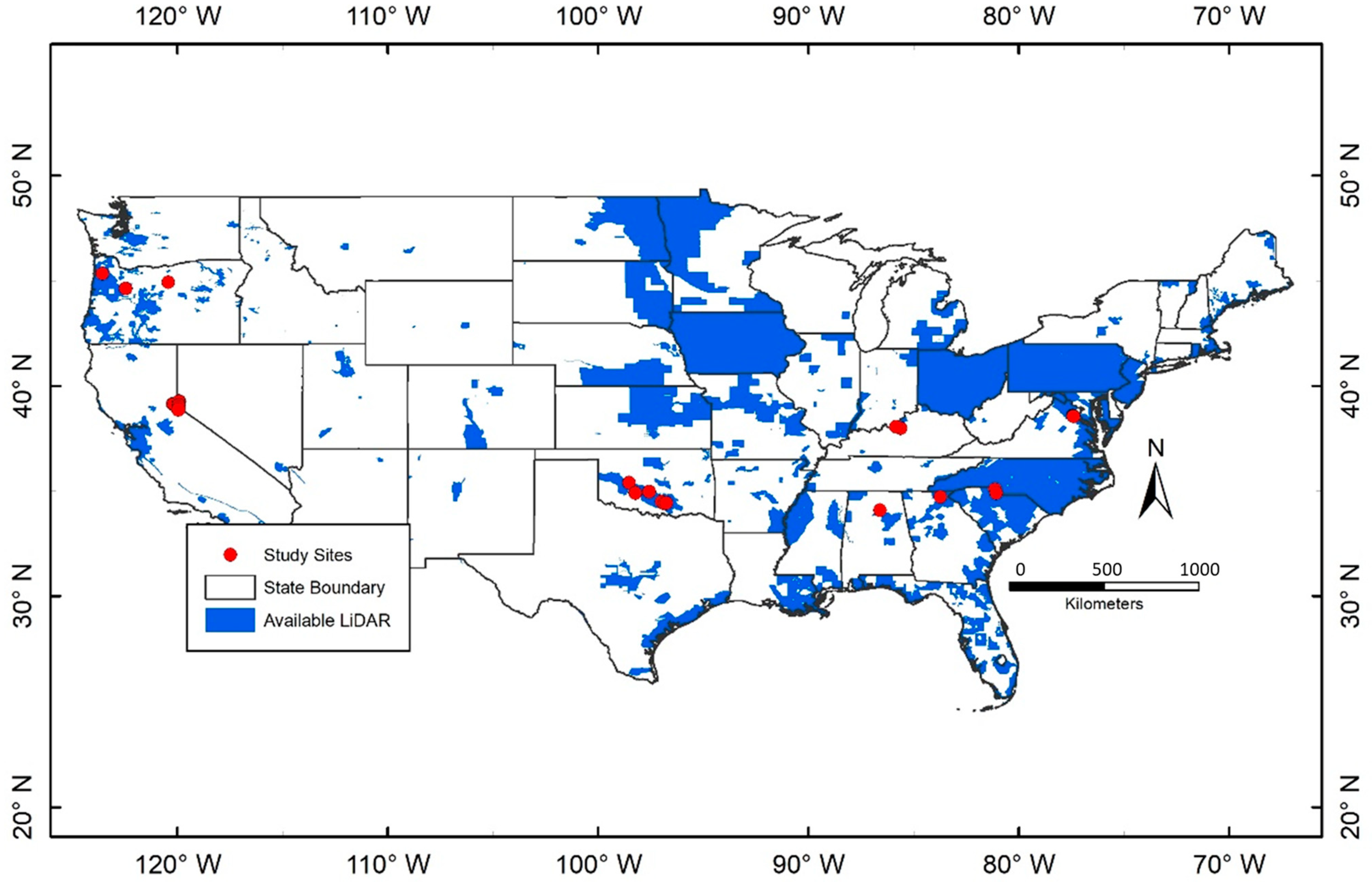
2. Data and Methodology

A total of 30 study watersheds, located across ten states in the United States, were selected based on the availability of both LiDAR data and streamflow observations, as shown in Figure 1. LiDAR data were obtained through the USGS Center for LiDAR Information, Coordination and Knowledge (CLICK) website (http://lidar.cr.usgs.gov, accessed on 20 August 2015), and the data quality varied for each LiDAR dataset. The LiDAR acquisition dates for each watershed and the corresponding average daily streamflow, from the USGS streamgage at the downstream outlet of each watershed, during the acquisition period are listed in

Table 1. United States Geological Survey (USGS) gage identification number, drainage area, climate aridity index, streamflow during the lidar survey, and its exceedance probability during the LiDAR surveys for the study watersheds. [E_p/P: climate aridity index as the ratio of annual potential evaporation (E_p) to precipitation (P), E_Q: exceedance probability of streamflow].

Watershed	USGS Gage	Drainage Area (km2)	${\mathit{E}}_{\mathit{P}}/\mathit{P}$	LiDAR Acquisition Date	Streamflow (m3/s)	${\mathit{E}}_{\mathit{Q}}$ (%)
Tucca Creek, OR	14303200	6.0	0.3	9 May 2010 ~13 May2010	0.481 ± 0.11	28
Schafer Creek, OR	14188610	5.5	0.4	9 October 2012	0.001	98
Chattahoochee River, GA	02330450	116.2	0.8	30 March 2010	4.474	27
Ward Creek, CA (Upstream)	10336674	12.0	0.9	14 August 2010	0.074	54
Blue Springs Creek, AL	02449882	31.4	0.9	26 February 2010	0.481	26
Cedar Creek, KY	03297800	31.2	1.0	21 March 2009	0.136	51
Brier Creek, KY	03302050	10.5	1.0	20 March 2009	0.037	47
Blackwood Creek, CA	10336660	28.9	1.0	20 August 2010 ~23 August 2010	0.103 ± 0.01	73
				20 June 2012 ~21 June 2012	0.524 ± 0.01	40
Ward Creek, CA	10336676	24.9	1.0	14 August 2010	0.057	72
				20 June 2012 ~21 June2012	0.27 ± 0.01	43
South Fork Quantico Creek, VA	01658500	19.4	1.0	7 April 2011 ~14 April 2011	0.194 ± 0.03	22
Middle Branch Chopawamsic Creek, VA	01659500	11.4	1.1	7 April 2011	0.096	28
North Branch Chopawamsic Creek, VA	01659000	15.0	1.1	7 April 2011	0.125	26
South Branch Chopawamsic Creek, VA	01660000	6.5	1.1	6 April 2011 ~7 April2011	0.057 ± 0.01	45
General Creek, CA	10336645	19.2	1.1	20 August 2010 ~23 August 2010	0.020	95
Allison Creek, SC	021457492	104.0	1.1	12 March 2012	0.425	34
Wildcat Creek, SC	021473428	76.6	1.1	8 March 2011	0.453	20
Pennington Creek, OK	07331295	85.2	1.3	22 December 2009 ~26 December 2009	0.580 ± 0.04	28
Mill Creek, OK	07331200	120.9	1.3	22 December 2009	0.255	26
Rock Creek, OK	07329852	114.3	1.3	22 December 2009	0.651	33
Incline Creek, NV (Upstream)	103366993	7.4	1.4	12 August 2010	0.040	74
North Criner Creek, OK	07328180	18.6	1.5	20 December 2009	0.006	67
Incline Creek, NV	10336700	17.3	1.5	12 August 2010	0.099	66
Trout Creek, CA	10336770	19.1	1.6	23 August 2010	0.156	54
Little Washita River, OK	07327442	36.5	1.6	17 December 2009	0.071	41
Little Washita River, OK (Upstream)	073274406	9.3	1.6	17 December 2009	0.015	45
Lake Creek, OK	07325840	49.4	1.7	13 December 2009	0.176	18
Logan House Creek, NV	10336740	5.3	1.9	16 August 2010 ~17 August 2010	0.002	87
Glenbrook Creek, NV	10336730	10.3	2.1	16 August 2010 ~18 August 2010	0.005	88
Eagle Rock Creek, NV	103367592	1.5	2.1	16 August 2010 ~17 August 2010	0.014	75
Pine Creek near Clarno, OR	14046890	336.9	2.7	19 May 2011 ~20 May 2011	0.368	7

. The LiDAR survey years for the study watersheds range from 2009 to 2012. As the LiDAR datasets used in this study were acquired before the 3D Elevation Program was established, the minimum specification and five quality levels were not indicated [31]. The intensity map and the land surface topography were derived from the LiDAR point cloud data using the QCoherent LP360 toolbox for ArcGIS (https://www.lp360.com/, accessed on 20 August 2015).

The drainage area, climate aridity index ($E_P/P$), streamflow variation, and streamflow exceedance probability ($E_Q$) during the LiDAR acquisition day are summarized in Table 1, and the watersheds are arranged by the climate aridity index from the smallest (0.3) to the largest (2.7). Streamflow observations were acquired from the USGS National Water Information System (http://waterdata.usgs.gov/nwis, accessed on 3 January 2023). $E_Q$ was defined as the probability that a specific streamflow will be achieved and exceeded for each watershed by generating a flow duration curve based on the daily streamflow records from USGS gages. The $E_Q$ for the study watersheds ranged from 7% (high flow) to 98% (low flow). For example, the $E_Q$ of Shafer Creek and General Creek were 98% and 95%, respectively, indicating a low flow condition when extensive dry channels were expected.

The climate aridity index, defined as the ratio of annual potential evaporation to precipitation ($E_P/P$), was used as a numerical indicator of the climate in a watershed [30,32]. Except for Tucca Creek (0.3), Schafer Creek (0.4), and Pine Creek (2.7), the climate aridity index for the study watersheds varied from 0.8 to 2.1. Perennial streams were obtained from the National Hydrography Dataset (NHD) [33]. The flowing channel networks corresponding to certain streamflow exceedance probabilities were compared with NHD perennial streams to evaluate the determination of perennial stream.

The key component of the LiDAR data for identifying wet channels was the signals’ intensity of ground returns. The signals’ intensity is a relative measurement of the return strength of a laser pulse received by a LiDAR sensor. LiDAR systems operate in the near-infrared (NIR) range, and the absorption of NIR signals by water is significantly higher than that of dry land [34]. This characteristic of NIR leads to the fact that LiDAR return intensities over water surfaces are relatively low compared with those of dry lands such as dry channels and hillslopes.

Figure 2 shows the intensity map for a headwater catchment in Ward Creek. Intensity is encoded as a digital number (DN), which is the raw values recorded by the sensor. Wet channels show consistently lower intensities and continuous patterns compared to other locations, such as hill slopes and dry channels. Wet channel heads, which are the starting points of wet channels, are visually detected and displayed by a blue dot.

This study follows the methodology developed by Hooshyar et al. [28], which is a systematic method for wet channel network extraction by integrating LiDAR intensity with a digital elevation model (DEM). In this study, intensity maps and DEMs with 1-m spatial resolution were generated. This method was based on several major steps. First, densely vegetated areas in the intensity map were filtered out because the return intensity from the ground points under the canopy was typically low regardless of wetness, and their inclusion could lead to false positives. This was accomplished by filtering out any pixels in which the difference between the ground and canopy elevations was more than 2 m. The second step was to extract the valley network and extent from the LiDAR-based 1-m DEM. Wet channels are located within the valley networks where individual valleys are associated with positive contour curvature. A small positive curvature threshold (0.025 m⁻¹) was used to generate the valley extents from the DEM.

Figure 3 shows a contour curvature map and the identified valley extent determined by the curvature threshold in a sub-catchment of the Ward Creek watershed. The third step was to decompose the composite probability distribution function (PDF) of intensity. The general PDF of intensity consists of several Gaussian distributions, and each distribution corresponds to a ground surface category, such as wet or dry conditions. The intensity thresholds for classifying wet pixels were extracted from the PDF analysis on points within the valley extent using a Gaussian mixture model [35]. Based on the individual PDFs, we identified valleys to differentiate wet, transition, and dry surfaces. The fourth step was to detect edges corresponding to high gradient pixels in the intensity map using Canny’s method [36] to improve the identification of small wet channels. Finally, the wet channel network was generated by combining wet pixels based on the intensity thresholds and the detected edges. Isolated segments of the resulting wet channels were manually connected. Figure 4a shows the identified wet pixels, and Figure 4b shows the connected wet channel network and the valley network after processing isolated wet channel segments in the Ward Creek watershed. The connected wet channel and valley network of all of the study watersheds are shown in Supplementary Figure S1. More details regarding the methodology can be found in Hooshyar et al. [28].

3. Results and Discussion

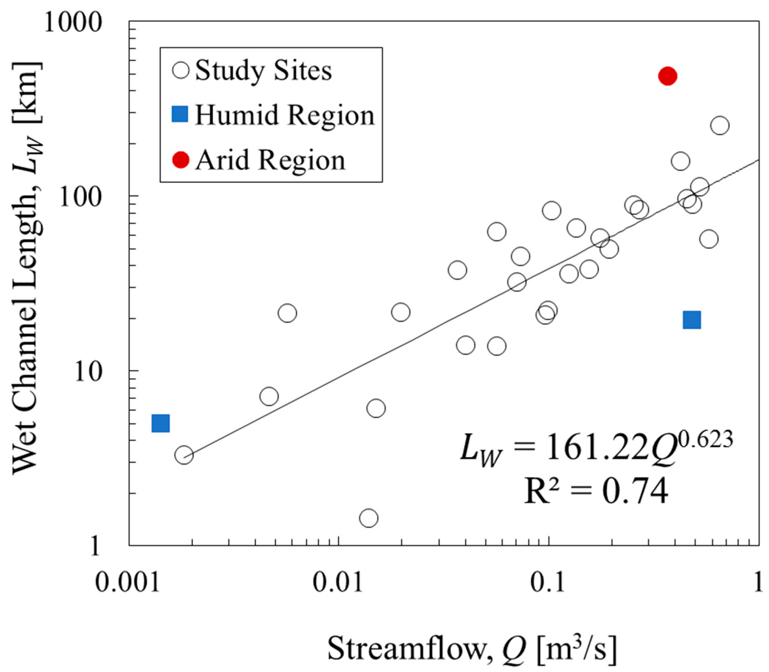
3.1. The Relationship between the Wet Channel Length and Streamflow

In this study, we applied Hooshyar et al. [28]’s method to all of the study watersheds using LiDAR-based DEM and intensity data in order to extract valley networks and identify wet channels. The wet channel length increases with the streamflow and has been described by an empirical power–law function based on field observations. This has been proven to be effective in quantifying this relationship, as reported by Blyth and Rodda [37], Godsey and Kirchner [38], and Whiting and Godsey [39]. Hooshyar et al. [28] also corroborated that the power–law relationship holds when using wet channels identified by integrating LiDAR intensity and elevation data. The scaling exponent of the power–law relationship can be unique to the season (e.g., wet or dry) [37,40] and the position in the hydrograph (e.g., rising or recession limbs) [41]. This is due to the dependence of the wet channel network on the local watershed properties such as precipitation, soil, vegetation, and topography [42,43,44,45].

The relationship between wet channel length ($L_W$) and streamflow (Q) for the study watersheds is plotted in Figure 5, and the total valley length, wet channel length, and wet channel ratio are listed in Supplementary Table S1, organized in the climate aridity index ($E_P/P$) from the smallest to the largest. Three watersheds were excluded from the data as they were excessively humid ($E_P/P$: 0.3~0.4) and arid ($E_P/P$: 2.7), and they displayed uncharacteristic patterns of wet channel length and streamflow patterns. The range of $E_P/P$ was 0.8 to 2.1 for the remaining 27 watersheds with 29 LiDAR snapshots, and the best fit function was $L_W$ = 161.22Q^0.623 with R² = 0.74, as shown in Figure 5. The scaling exponent of the power–law relationship (i.e., 0.623) was within the range of the reported values (i.e., 0.042~0.688) in the literature from fieldwork conducted in 14 watersheds in other regions [38].

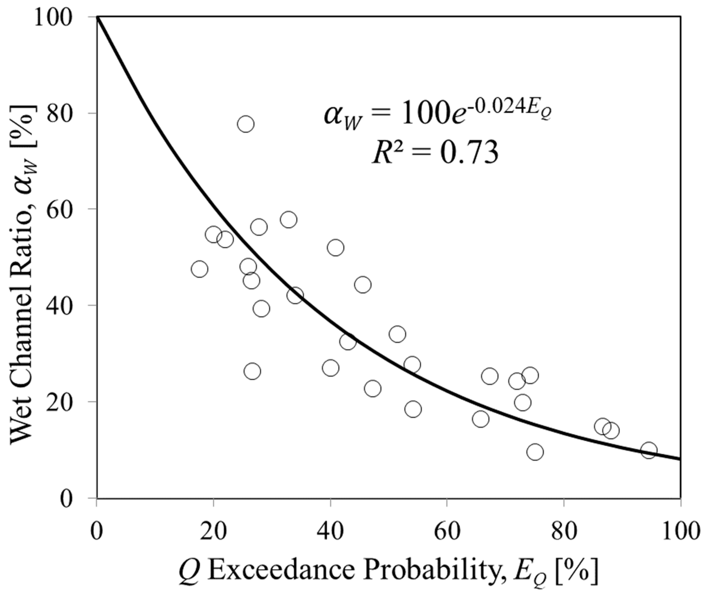
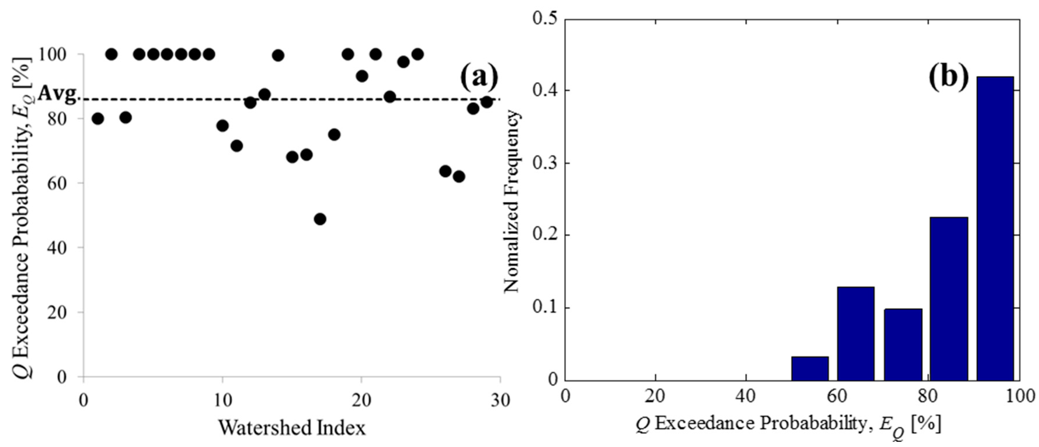
3.2. The Relationship between the Wet Channel Ratio and Streamflow Exccedance Probability

To better understand the definition of perennial streams, the relationships between two non-dimensional variables were investigated (Figure 6): streamflow exceedance probability ($E_Q$) and the wet channel ratio (${\alpha }_W$). $E_Q$ values of 0% and 100% represented the highest and lowest streamflows, respectively. An $E_Q$ of 0% was likely to be an underestimation as it was evaluated based on limited streamflow data. Despite this fact, it was assumed that all of the stream networks were flowing (i.e., ${\alpha }_W$ = 100%) when the maximum streamflow occurred (i.e., $E_Q$ = 0%). Under this assumption, the best fit function was an exponential function,${\alpha }_W=100e^{-0.024E_Q}$ with R² = 0.73, as shown in Figure 6.

From the fitted equation, an $E_Q$ of 100% (i.e., the minimum streamflow) corresponded to an ${\alpha }_W$ of 9.1%. Using the definition of a perennial stream from the literature, $E_Q$ values of 90% and 80% corresponded to ${\alpha }_W$ values of 11.4% and 14.7%, respectively. Wang and Wu [46] showed that perennial stream density declines from around 0.6 km/km² to 0.2 km/km² since the minimum streamflow decreases when $E_P/P$ increases from 0.8 to 2.1 (i.e., less rainfall). The drainage density slightly increases (around 9~13 km/km²) for $0.8\le E_P/P\le 2.1$ based on the dependence of drainage density on the climate. Therefore, the perennial stream ratio (PSR), defined as the perennial stream length over the total valley length, declines with $E_P/P$ for a perennial stream.

The perennial stream length of each watershed was obtained from the National Hydrography Dataset (NHD), and the valley length was extracted from LiDAR DEM to compute the perennial stream ratio (PSR). As shown in Figure 7a, the $E_Q$ of the perennial streamflow for each watershed was calculated using the relationship between $E_Q$ and ${\alpha }_W$, as shown in Figure 6. The range of the perennial stream ratio (PSR) for the study watersheds was 1.2% to 29.4% with a mean of 11.0%; the range of $E_Q$ corresponding to the perennial streamflow was from 49% to 100%, and the average value was 86%. Figure 7b shows the distribution of perennial streamflow $E_Q$ for the study watersheds. The distribution was represented by normalized frequency, defined as the ratio of the number of watersheds in each bin to the total number of watersheds. Corresponding to the perennial streamflow, 71% of the study watersheds had $E_Q$ values greater than 80%.

The perennial streamflow for each watershed was directly calculated from the perennial stream length using the relationship between streamflow (Q) and wet channel length ($L_W$) in Figure 5. Subsequently, another $E_Q$ of perennial streamflow was computed using the flow duration curve for each watershed. The range of $E_Q$ regarding perennial streamflow was from 51% to 100%, and the average value was 88%. The ranges of $E_Q$ associated with perennial streamflow were similar using both relationships, and the mean values were 86% and 88%, respectively, which were in the range of the reported values (i.e., 80% and 90%) from the literature [7,8,9]. However, caution should be exercised when using the mean $E_Q$ value to define perennial streams because $E_Q$ values associated with perennial streamflow depend on the characteristics of the watershed, such as groundwater, land use, soil, vegetation, and topography. The NHD perennial stream lengths (PSR), perennial streamflows, and the $E_Q$ values for the perennial streamflows for the study watersheds are listed in

Table 2. National Hydrography Dataset (NHD) perennial stream length, stream ratio, streamflow, and $E_Q$ of the perennial streamflow for the study watersheds.

Watershed.	NHD Perennial Stream Length (km)	Perennial Stream Ratio (%)	Perennial Streamflow (m3/s)	(i) ${\mathit{E}}_{\mathit{Q}}$ of Perennial Streamflow (%)	(ii) ${\mathit{E}}_{\mathit{Q}}$ of Perennial Streamflow (%)
Chattahoochee River, GA	167.5	13.50	1.1541	80	90
Ward Creek, CA (Upstream)	5.5	3.33	0.0037	100	97
Blue Springs Creek, AL	25.2	13.40	0.0478	80	78
Cedar Creek, KY	2.3	1.22	0.0009	100	100
Brier Creek, KY	7.1	4.27	0.0056	100	72
Blackwood Creek, CA (2010)	24.8	5.96	0.0466	100	95
Blackwood Creek, CA (2012)	24.8	5.95	0.0466	100	95
Ward Creek, CA (2010)	15.0	5.81	0.0199	100	90
Ward Creek, CA (2012)	15.0	5.81	0.0199	100	90
South Fork Quantico Creek, VA	13.2	14.27	0.0161	78	80
Middle Branch Chopawamsic Creek, VA	8.8	16.69	0.0082	72	90
North Branch Chopawamsic Creek, VA	9.5	11.95	0.0092	85	87
South Branch Chopawamsic Creek, VA	3.5	11.18	0.0017	88	99
General Creek, CA	18.1	8.27	0.0272	100	84
Allison Creek, SC	68.3	18.16	0.2551	68	51
Wildcat Creek, SC	31.6	17.87	0.0698	69	72
Pennington Creek, OK	29.9	29.38	0.0636	49	96
Mill Creek, OK	17.5	15.25	0.0259	75	96
Rock Creek, OK	9.9	2.26	0.0099	100	100
Incline Creek, NV (Upstream)	5.4	9.70	0.0036	93	100
North Criner Creek, OK	3.8	4.46	0.0020	100	77
Incline Creek, NV	15.3	11.42	0.0207	87	100
Trout Creek, CA	18.1	8.68	0.0273	98	100
Little Washita River, OK	1.6	2.51	0.0004	100	95
Lake Creek, OK	24.5	20.28	0.0455	64	59
Logan House Creek, NV	4.7	21.18	0.0028	62	73
Glenbrook Creek, NV	6.4	12.49	0.0047	83	88
Eagle Rock Creek, NV	1.8	11.86	0.0005	85	100

(i) $E_Q$ of the perennial stream using the relationship between the wet channel ratio (${\alpha }_W$) and streamflow exceedance probability ($E_Q$). (ii) $E_Q$ of the perennial stream using the relationship between streamflow (Q) and wet channel length ($L_W$).

.

3.3. Temporal Variability

There are two watersheds where temporal variability was investigated by using LiDAR data from 2010 and 2012: Blackwood Creek, CA, and Ward Creek, CA. The perennial stream ratio (PSR) values computed using the NHD perennial stream lengths had little to no change from 2010 to 2012 (Table 2). In contrast, the wet channel lengths were increased in 2012 using this study’s approach by 30.3 km and 21.1 km, respectively (Table S1). This resulted in an increase in the wet channel ratio (${\alpha }_W$) from 19.9% to 27.1% and from 24.4% to 32.6%, respectively. The increase in the wet channel ratio (${\alpha }_W$) is the result of the streamflow difference from two LiDAR survey periods (Table 1). The average daily streamflow increased from 0.103 m³/s to 0.524 m³/s and from 0.057 m³/s to 0.27 m³/s for the respective watersheds.

4. Summary and Conclusions

The purpose of this study was to define perennial streams using the dimensionless relationship between streamflow exceedance probability ($E_Q$) and the wet channel ratio (${\alpha }_W$) based on wet channel networks extracted from LiDAR data. Based on available LiDAR data and streamflow observations, 30 watersheds were selected, and the valley network and wet channels were extracted from LiDAR topographic data and the signals’ intensity of ground returns with a 1 m spatial resolution. The results of the study can be summarized as follows.

Using the observed streamflows and the wet channels identified, we derived a power–law relationship between wet channel length and streamflow; the scaling exponent of this relationship was within the range of values reported in the literature. This relationship was converted into a non-dimensional form using $E_Q$ and ${\alpha }_W$, and the previous definition of perennial streams using $E_Q$ values of 90% and 80% corresponded to ${\alpha }_W$ values of 11% and 15%, respectively. The perennial stream ratio was computed for each study watershed to validate the derived ${\alpha }_W$ associated with the perennial stream definition, and its mean value (i.e., 11%) was within the range of the ${\alpha }_W$ associated with the definition of perennial streams in this study. Moreover, the streamflow exceedance probability of perennial streamflow for each watershed was calculated, and its mean value (86%) was similar to previous definition values (i.e., 80% and 90%).

Although this study attempted to define the perennial stream with relatively limited watershed and LiDAR information, the relationship between streamflow exceedance probability and the wet channel ratio showed significant agreement with previous studies on perennial stream definition. In addition, the results clearly demonstrated the possibility of applying the wet channel ratio as another parameter for defining perennial streams. The relationships determined in this study are likely to be applicable in similar climates (e.g., climate aridity index $E_P/P$ = 0.8~2.1). However, more research is needed to consider other hydrologic factors, e.g., antecedent moisture conditions, precipitation, or potential evapotranspiration, as well as vegetation conditions. Densely vegetated areas were filtered out due to their low signal intensity, and the proposed approach may not apply effectively in heavily forested areas. The proposed approach can also be applied to broader climate conditions and possibly identify intermittent and ephemeral streams.

The LiDAR data that were used to extract the valley networks in this study represent the ground and streamflow conditions only during the LiDAR acquisition period. In turn, temporal variability was evaluated using LiDAR data from two separate periods for two watersheds. Further investigations are suggested regarding the sensitivity of the perennial stream definition process depending on LiDAR acquisition time. The study watersheds were considered natural and undeveloped areas, and we used climate indices such as evapotranspiration and streamflow to understand the environmental effect of the perennial streams. Application of this technique is expected to have a positive impact on eco-hydrology and the environment management of perennial streams. We believe that the data extraction technique using high-precision and high-accuracy LiDAR-based DEM proposed in this study may provide a robust alternative to define perennial streams. The results of this study will provide useful data for more accurate watershed and streamflow modeling, ecological-environmental analysis, and for the management of floodplain restoration.

References

1. Meinzer, O.E. Outline of ground-water hydrology, with definitions. US Govt. Print. Off. 1923, 494, 1–68. [Google Scholar]
2. Von Schiller, D.; Acuña, V.; Sabater, S. Wetlands and Habitats, 2nd ed.; Streams: Perennial and seasonal; CRC Press: Boca Raton, FL, USA, 2020; ISBN 978-04-2944-550-7. [Google Scholar]
3. Chow, V.T.; Maidment, D.R.; Mays, L.W. Applied Hydrology; McGraw Hill: New York, NY, USA, 1988. [Google Scholar]
4. Blasch, K.W.; Ferré, T.; Christensen, A.H.; Hoffmann, J.P. New field method to determine streamflow timing using electrical resistance sensors. Vadose Zone J. 2002, 1, 289–299. [Google Scholar] [CrossRef]
5. Levick, L.R.; Goodrich, D.C.; Hernandez, M.; Fonseca, J.; Semmens, D.J.; Stromberg, J.C.; Tluczek, M.; Leidy, R.A.; Scianni, M.; Guertin, D.P. The Ecological and Hydrological Significance of Ephemeral and Intermittent Streams in the Arid and Semi-Arid American Southwest; US Environmental Protection Agency, Office of Research and Development: Washington, DC, USA, 2008.
6. NC Division of Water Quality. Methodology for Identification of Intermittent and Perennial Streams and Their Origins, Version 4.11; North Carolina Department of Environment and Natural Resources, Division of Water Quality: Raleigh, NC, USA, 2010. [Google Scholar]
7. Hedman, E.; Osterkamp, W. Streamflow Characteristics Related to Channel Geometry of Streams in Western United States; Water Supply Paper 2193; US Geological Survey: Alexandria, VA, USA, 1982.
8. Hewlett, J.D. Principles of Forest Hydrology; University of Georgia Press: Athens, GA, USA, 1982. [Google Scholar]
9. Texas Forest Service. Texas Forestry Best Management Practices. Online Report. 2000. Available online: https://tfsweb.tamu.edu/uploadedFiles/TFSMain/Manage_Forest_and_Land/Water_Resources_and_BMPs/Stewardship(1)/BMP%20Handbook_clean%20copy,%20Aug%202017.pdf (accessed on 3 January 2023).
10. Schumm, S.A. Evolution of drainage systems and slopes in badlands at Perth Amboy, New Jersey. Geol. Soc. Am. Bull. 1956, 67, 597–646. [Google Scholar] [CrossRef]
11. Howard, A.D.; Kerby, G. Channel changes in badlands. Geol. Soc. Am. Bull. 1983, 94, 739–752. [Google Scholar] [CrossRef]
12. Simley, J. National Hydrography Dataset Newsletter. US Geol. Surv. Rep. 2003, 2. Available online: http://nhd.usgs.gov/newsletterlist.html (accessed on 3 January 2023).
13. Svec, J.R.; Kolka, R.; Stringer, J. Defining perennial, intermittent, and ephemeral channels in eastern Kentucky: Application to forestry best management practices. For. Ecol. Manag. 2005, 214, 170–182. [Google Scholar] [CrossRef]
14. Jaeger, K.L.; Sando, R.; McShane, R.R.; Dunham, J.B.; Hockman-Wert, D.P.; Kaiser, K.E.; Hafen, K.; Risley, J.C.; Blasch, K.W. Probability of Streamflow Permanence Model (PROSPER): A spatially continuous model of annual streamflow permanence throughout the Pacific Northwest. J. Hydrol. X 2019, 2, 100005. [Google Scholar] [CrossRef]
15. Marks, K.; Bates, P. Integration of high-resolution topographic data with floodplain flow models. Hydrol. Process. 2000, 14, 2109–2122. [Google Scholar] [CrossRef]
16. Bowen, Z.H.; Waltermire, R.G. Evaluation of light detection and ranging (LIDAR) for measuring river corridor topography. J. Am. Water Resour. Assoc. 2002, 38, 33–41. [Google Scholar] [CrossRef]
17. Lashermes, B.; Foufoula-Georgiou, E.; Dietrich, W.E. Channel network extraction from high resolution topography using wavelets. Geophys. Res. Lett. 2007, 34, L23S04. [Google Scholar] [CrossRef] [Green Version]
18. Orlandini, S.; Moretti, G. Determination of surface flow paths from gridded elevation data. Water Resour. Res. 2009, 45, W03417. [Google Scholar] [CrossRef] [Green Version]
19. Orlandini, S.; Tarolli, P.; Moretti, G.; Dalla Fontana, G. On the prediction of channel heads in a complex alpine terrain using gridded elevation data. Water Resour. Res. 2011, 47, W02538. [Google Scholar] [CrossRef]
20. Sofia, G.; Tarolli, P.; Cazorzi, F.; Dalla Fontana, G. An objective approach for feature extraction: Distribution analysis and statistical descriptors for scale choice and channel network identification. Hydrol. Earth Syst. Sci. 2011, 15, 1387–1402. [Google Scholar] [CrossRef] [Green Version]
21. Pelletier, J.D. A robust, two-parameter method for the extraction of drainage networks from high-resolution digital elevation models (DEMs): Evaluation using synthetic and real-world DEMs. Water Resour. Res. 2013, 49, 75–89. [Google Scholar] [CrossRef] [Green Version]
22. Clubb, F.J.; Mudd, S.M.; Milodowski, D.T.; Hurst, M.D.; Slater, L.J. Objective extraction of channel heads from high-resolution topographic data. Water Resour. Res. 2014, 50, 4283–4304. [Google Scholar] [CrossRef] [Green Version]
23. Metes, M.J.; Jones, D.K.; Baker, M.E.; Miller, A.J.; Hogan, D.M.; Loperfido, J.V.; Hopkins, K.G. Ephemeral stream network extraction from Lidar-derived elevation and topographic attributes in urban and forested landscapes. J. Am. Water Resour. Assoc. 2022, 58, 547–565. [Google Scholar] [CrossRef]
24. Genc, L.; Smith, S.E.; Dewitt, B.A. Using satellite imagery and lidar data to corroborate an adjudicated ordinary high water line. Int. J. Remote Sens. 2005, 26, 3683–3693. [Google Scholar] [CrossRef]
25. Höfle, B.; Vetter, M.; Pfeifer, N.; Mandlburger, G.; Stötter, J. Water surface mapping from airborne laser scanning using signal intensity and elevation data. Earth Surf. Process. Landf. 2009, 34, 1635–1649. [Google Scholar] [CrossRef]
26. Smeeckaert, J.; Mallet, C.; David, N.; Chehata, N.; Ferraz, A. Large-scale classification of water areas using airborne topographic lidar data. Remote Sens. Environ. 2013, 138, 134–148. [Google Scholar] [CrossRef]
27. Wu, H.; Liu, C.; Zhang, Y.; Sun, W.; Li, W. Building a water feature extraction model by integrating aerial image and lidar point clouds. Int. J. Remote Sens. 2013, 34, 7691–7705. [Google Scholar] [CrossRef]
28. Hooshyar, M.; Kim, S.; Wang, D.; Medeiros, S.C. Wet channel network extraction by integrating LiDAR intensity and elevation data. Water Resour. Res. 2015, 51, 10029–10046. [Google Scholar] [CrossRef]
29. Liu, C.; Wang, L.; Xin, Z.; Li, Y. Comparative study of wet channel network extracted from LiDAR data under different climate conditions. Hydrol. Res. 2018, 49, 1101–1119. [Google Scholar] [CrossRef]
30. Zambory, L.C.; Ellis, H.; Pierce, L.C.; Roe, J.K.; Weber, J.M.; Schilling, E.K.; Young, C.N. The Development of a GIS Methodology to Identify Oxbows and Former Stream Meanders from LiDAR-Derived Digital Elevation Models. Remote Sens. 2019, 11, 12. [Google Scholar] [CrossRef] [Green Version]
31. Budyko, M.I. The Heat Balance of the Earth’s Surface; US Department of Commerce: Washington, DC, USA, 1958.
32. Heidemann, H.K. Lidar Base Specification (ver. 1.3, February 2018): U.S. Geological Survey Techniques and Methods; U.S. Geological Survey: Sioux Falls, SD, USA, 2018; Book 11; Chapter B4; 101p. [CrossRef] [Green Version]
33. National Hydrography Dataset Homepage. Available online: https://www.usgs.gov/national-hydrography/national-hydrography-dataset (accessed on 6 November 2022).
34. Wolfe, W.L.; Zissis, G.J. The Infrared Handbook; ERIM: Rotterdam, The Netherlands, 1989; pp. 1124–1127. [Google Scholar]
35. Rasmussen, C.E. The infinite Gaussian mixture model. In Advances in Neutral Information Processing Systems 12; MIT Press: Cambridge, MA, USA, 2000. [Google Scholar]
36. Canny, J. A Computational approach to edge detection. IEEE Trans. Pattern Anal. Mach. Intell. 1986, PAMI–8, 679–698. [Google Scholar] [CrossRef]
37. Blyth, K.; Rodda, J. A stream length study. Water Resour. Res. 1973, 9, 1454–1461. [Google Scholar] [CrossRef]
38. Godsey, S.; Kirchner, J. Dynamic, discontinuous stream networks: Hydrologically driven variations in active drainage density, flowing channels and stream order. Hydrol. Process. 2014, 28, 5791–5803. [Google Scholar] [CrossRef]
39. Whiting, J.A.; Godsey, S.E. Discontinuous headwater stream networks with stable flowheads, salmon river basin, Idaho. Hydrol. Process. 2016, 30, 2305–2316. [Google Scholar] [CrossRef]
40. Wigington, P.; Moser, T.; Lindeman, D. Stream network expansion: A riparian water quality factor. Hydrol. Process. 2005, 19, 1715–1721. [Google Scholar] [CrossRef]
41. Roberts, M.C.; Archibold, O. Variation of Drainage Density in a Small British Columbia Watershed; Wiley Online Library: Hoboken, NJ, USA, 1978. [Google Scholar]
42. Morgan, R.P.C. Observations on factors affecting the behaviour of a first-order stream. Trans. Ins. Brit. Geogr. 1972, 56, 171–185. [Google Scholar] [CrossRef]
43. Day, D.G. Drainage density changes during rainfall. Earth Surf. Process. 1978, 3, 319–326. [Google Scholar] [CrossRef]
44. Gurnell, A.M. The dynamics of a drainage network. Nord. Hydrol. 1978, 9, 293–306. [Google Scholar] [CrossRef]
45. Goulsbra, C.; Evans, M.; Lindsay, J. Temporary streams in a peatland catchment: Pattern, timing, and controls on stream network expansion and contraction. Process. Landf. 2014, 39, 790–803. [Google Scholar] [CrossRef]
46. Wang, D.; Wu, L. Similarity of climate control on base flow and perennial stream density in the Budyko framework. Hydrol. Earth Syst. Sci. 2013, 17, 315–324. [Google Scholar] [CrossRef]
Figure 1. Location of study sites and available LiDAR data. The red dots indicate a total of 30 study watersheds across the ten states and the blue dots means the availability of LiDAR raw point data in the United States as of 2015.
Applsci 13 00704 g001
Figure 2. Intensity image during 2012 LiDAR survey for a headwater area in the Ward Creek watershed. The blue dots visually identified the wet channel head [DN: digital number].
Applsci 13 00704 g002
Figure 3. A contour curvature map and the identified valley extent determined by the curvature threshold in a sub-catchment of the Ward Creek watershed. (a) The contour curvature and the visible detection of the drainage path determined by blue color pixels. (b) The intensity returns within the valley extent determined by the curvature threshold in the Ward Creek watershed in the 2012 LiDAR survey [DN: digital number].
Applsci 13 00704 g003
Figure 4. The identified wet pixels and the connected wet channel network with the valley network. (a) The identified wet pixels based on the intensity thresholds. (b) The connected wet channel network with the valley network after processing isolated wet channel segments based on the 2012 LiDAR survey in the Ward Creek watershed [DN: digital number].
Applsci 13 00704 g004
Figure 5. The relationship between streamflow (Q), presented in Table 1, and wet channel length ( L W ) in the study watersheds.
Applsci 13 00704 g005
Figure 6. The relationship between streamflow exceedance probability ( E Q ) and the wet channel ratio ( α W ) in the study watersheds.
Applsci 13 00704 g006
Figure 7. Streamflow exceedance probability of the perennial streams and its normalized frequency distribution. (a) Streamflow exceedance probability ( E Q ) of the perennial streams in the study watersheds using the relationship between the wet channel ratio ( α W ) and E Q ; and (b) normalized frequency distribution of E Q for all of the study sites.
Applsci 13 00704 g007