Classifying Images of Two-Dimensional Fractional Brownian Motion through Deep Learning and Its Applications

Abstract

Two-dimensional fractional Brownian motion (2D FBM) is an effective model for describing natural scenes and medical images. Essentially, it is characterized by the Hurst exponent (H) or its corresponding fractal dimension (D). For optimal accuracy, we can use the maximum likelihood estimator (MLE) to compute the value. However, its computational cost is much higher than other low-accuracy estimators. Therefore, we propose a feasible deep-learning model and find out some promising pretrained models to classify the Hurst exponent efficiently and effectively. For evaluating the efficacy of deep learning models, two types of 2D FBM images were generated—11 classes and 21 classes of Hurst exponents. For comparison, we first used the efficient MLE to estimate the Hurst exponent of each image and then classified them through machine learning models. On the other hand, we used deep learning models to train and classify all images. Experimental results show that our proposed model and some pretrained models are much higher in accuracy than machine learning models for estimates from the efficient MLE. When applied, deep learning models take much lower computational time than the efficient MLE. Therefore, for accuracy and efficiency, we can use deep learning models to replace the role of the efficient MLE in the future.

1. Introduction

Fractal geometry plays a very important role in explaining irregular images (or surfaces) and signals, for example, a classification for pathological prostate images [1], a classification for solitary pulmonary nodules [2], an online detection method for dry coal screening [3], an evaluation of changes in the structure of modified cement composite [4], a temperature fluctuation prediction [5], and a stock prediction [6].

For fractal images and signals, we often use fractal dimension (FD) to describe irregular structures—a smoother image/signal is from a smaller FD and a rougher one from a larger FD. For example, the intensities of some medical images, especially for pathological tissues, can be modeled as fractal images. In general, the textures of malignant tissues, such as nodules, are rougher than those of benign tissues, and more serious ones appear much rougher. Therefore, we can use the FD as an indicator to distinguish between benign and malignant tissues.

Among models to describe fractal images or irregular ones with self-similarity, two-dimensional fractional Brownian motion (2D FBM) [7,8] is often adopted because it can give physical meanings to explain the characteristics of images. Furthermore, two-dimensional fractional Gaussian noise (2D FGN)—the corresponding two-dimensional derivative process of 2D FBM—can be used to describe much rougher images. These two models can also be appropriate to describe some natural scenes [9,10,11].

These two models contain only one parameter—the Hurst exponent (H), a real value between 0 and 1—to distinguish between characteristics of various images; it is directly related to the FD (D) via D = 3 − H [7]. The Hurst exponent is limited, and hence it suitably serves as an effective feature; in addition, its value between 0 and 1 is particularly suitable for mapping or transforming an original image to a feature image or map. For machine learning or deep learning on certain images, we can provide this feature as an extra input to improve the classification rate.

Generally, the efficacy of the extra feature—the Hurst exponent—depends on the estimation accuracy because the higher the estimation accuracy is, the better the classification rate. Therefore, it is very important to find out the best estimator of the Hurst exponent as our auxiliary tool. Related estimators are calculated through the fractal Brownian surface [12], the Fourier power spectrum [13], the reticular cell counting [14], the differential box-counting [15,16,17,18,19,20], and the blanket [21].

Recently, Chang [22] proposed the maximum likelihood estimator (MLE)—the best estimator—for the 2D FBM images. It is an unbiased estimator and has the smallest mean-squared error. Therefore, we are pleased to adopt the MLE for 2D FBM images to estimate the Hurst exponent or its corresponding fractal dimension. On the one hand, we can directly use these estimates to differentiate between different images or tissues; on the other hand, we also can use these estimates as a feature to classify them through machine learning models.

In the past, when surfaces or images were modeled as 2D FBM—the former is called 2D FBM surfaces and the latter 2D FBM images, we estimated their Hurst exponents or their corresponding fractal dimensions through estimators and then used these values or estimates as an index or indicator.

However, any estimator, even the best estimator—the MLE—more or fewer results in error, and hence their estimates are not completely reliable. In addition, although the best estimator can obtain the most accurate estimate, its computational time is still high even though it has lowered much by an efficient MLE [22].

As deep learning models have continued to flourish over the years, another novel and practical point of view emerged that estimates might be calculated from deep learning models, not traditional estimators.

In the paper, we adopt another way to express the indicator of the Hurst exponent—the class of the Hurst exponent—instead of the value of the Hurst exponent. In fact, however, a class of the Hurst exponent can be viewed as an equivalent estimate with a fixed interval, say, 0.1.

To understand the tolerable spacing between two Hurst exponents, two resolutions—11 and 21 classes or Hurst exponents with equal intervals—will be considered. For each resolution, we first estimate Hurst exponents of 2D FBM images via the efficient MLE. Next, we use the estimated Hurst exponents as the only feature to train and further classify them through machine learning models. Finally, a classification report will be provided—hence, its resolution will be implied.

Based on the same data or images as machine learning models, we use the original images—not the estimated Hurst exponents—to train deep learning models and then classify them. Finally, a classification report will also be provided.

The paper is composed of two main purposes. The first aim is to see whether deep learning models on the FBM images have any possibilities to surpass the traditional way—that is, machine-learning models are run on the only feature of the estimated Hurst exponents of 2D FBM images. If successful, the second aim is to apply theses promising deep learning models to recognize the classes of images—or equivalently estimate Hurst exponents of images.

Among artificial intelligence methods, machine learning analyzes data through algorithms, understand the content of the data, and then applies the learned knowledge to determine other data and make appropriate decisions. Deep learning is a branch of machine learning. It uses the concept of “layers” to construct learning models that can automatically learn and then make intelligent decisions. Although deep learning belongs to machine learning, their functions are different. Deep learning can perform artificial intelligence functions that approximate the logic of human thinking as closely as possible; however, machine learning still needs human intervention and guidance. In the deep learning model, the algorithm can determine whether or not the prediction result is accurate. If the algorithm returns inaccurate predictions, its developer will step in and retrain the proposed model [23].

For better results, deep learning requires a large amount of data. Fortunately, with the advancement of modern computer technology, the acquisition and collection of data at present are more efficient than in the past. However, if the amount of data is not enough, the performance of deep learning, in general, will not be very good. Relatively, machine learning requires more resources than deep learning. For example, before performing machine learning, we need to extract some useful features from the original data and then use these features to train models.

Besides, in the past, deep learning models were run under central processing units (CPUs), and hence they take a very long time to train. As the technology of graphics processing units (GPUs) gets mature, deep learning models have become more efficient. Hence, GPUs have gradually become the mainstream of artificial intelligence [24].

In the paper, we will apply four machine-learning methods and four deep-learning models to compare and explore the classification of 2D FBM images. For machine learning [25,26], we use logistic regression (LR) for classification—simply called LR, support vector machines (SVMs), K-nearest neighbors (KNNs), and decision tree (DT). For deep learning [27,28,29], we will design a simple deep learning model and choose three pretrained models—AlexNet, GoogleNet, and Xception to evaluate their performances.

In the paper, Section 2 describes the materials and methods related to our study. Section 3 performs our experiments and works on the discussion. Applications through deep learning models for medical images are provided in Section 4. Finally, Section 5 concludes the paper with some facts and future works.

2. Materials and Methods

In this section, we will briefly introduce some related materials and methods. First, we will present the main materials: the process of 2D FBM (nonstationary) and its corresponding increment process, called 2D FGN (stationary), and then an estimator—the MLE for 2D FBM. Next, we introduced 4 machine learning models, including LR, SVMs, KNNs, and DT. Finally, we will explain 4 deep learning models, including our proposed simple sequential network, and 3 pretrained models—AlexNet, GoogleNet, and Xception.

2.1. Two-Dimensional Fractional Brownian Motion

Falconer [7] called the process of 2D FBM an index-H Brownian function; Hoefer et al. [30] called it isotropic 2D FBM, whose corresponding discrete version was called isotropic 2-dimensional discrete FBM; however, Balghonaim and Keller [31] called it as a 2-variable FBM, whose corresponding discrete version was called a 2-variable discrete fractional Brownian surface. For simplicity, we call it 2D FBM, and an image of 2D FBM is a 2D FBM image.

Suppose that an image of 2D FBM of size $M\times N$ is denoted as

$$I_B=\left[\begin{array}{cccc}B\left[0,0\right]& B\left[0,1\right]& \cdots & B\left[0,N-1\right]\\ B\left[1,0\right]& B\left[1,1\right]& \cdots & B\left[1,N-1\right]\\ ⋮& ⋮& \ddots & ⋮\\ B\left[M-1,0\right]& B\left[M-1,1\right]& \cdots & B\left[M-1,N-1\right]\end{array}\right]$$

(1)

For 2 coordinates or points $B\left[x_1, y_1\right]$ and $B\left[x_2, y_2\right]$, their ACF is as follows:

$$\begin{gathered} r_{BB}\left[\left(\begin{array}{c}{x}_1\\ y_1\end{array}\right), \left(\begin{array}{c}{x}_2\\ y_2\end{array}\right)\right]=E\left\{B\left[x_1, y_1\right]B\left[x_2, y_2\right]\right\} \\ =\frac{{\sigma }^2}{2}{‖\left(\begin{array}{c}{x}_1\\ y_1\end{array}\right)‖}^{2H}+{‖\left(\begin{array}{c}{x}_2\\ y_2\end{array}\right)‖}^{2H}-{‖\left(\begin{array}{c}{x}_1-x_2\\ y_1-y_2\end{array}\right)‖}^{2H}, \end{gathered}$$

(2)

where H is the Hurst exponent. Obviously, the ACF is directly related to the distance between 2 coordinates as well as 2 respective distances from the origin, and hence it is non-stationary.

For estimation, stationary ACFs are needed. Two approaches were proposed. The first was proposed by Hoefer et al. [30], who used the second increment process of 2D FBM to obtain a stationary covariance matrix. The resulting process is called 2-dimensional Gaussian noise (FGN2) [32] or simply called the first 2D FGN. The second was proposed by Balghonaim and Keller [31], who introduced another 2D FGN, simply called the second 2D FGN.

Chang [22] detailed these 2 2D FGNs and their related stationary covariances and symbols. Through the MLE, the mean-squared errors of the second 2D FGN are smaller than those of the first 2D FGN, but the first 2D FGN gives us more physical meanings because real surfaces or images may exist in the patterns of the first 2D FGN instead of the second 2D FGN.

Therefore, in the paper, we adopted the first 2D FGN to establish a probability density function (PDF) in order to estimate the Hurst exponent via the MLE. To obtain this 2D FGN, we first represent $I_B$ as a column vector of size $MN\times 1$ as follows:

$${\stackrel{\rightharpoonup }{B}}^T={\left[\begin{array}{cccc}{B}_0^T& B_1^T& \cdots & B_{M-1}^T\end{array}\right]}^{},$$

(3)

where

$$B_k^T=\left[\begin{array}{cccc}B\left[k,0\right]& B\left[k,1\right]& \cdots & B\left[k,N-1\right]\end{array}\right], k=0, 1,\dots , M-1.$$

Hence, its nonstationary covariance matrix is as follows:

$$R_{\stackrel{\rightharpoonup }{B}\stackrel{\rightharpoonup }{B}}=E\left\{\stackrel{\rightharpoonup }{B}{\stackrel{\rightharpoonup }{B}}^T\right\}$$

(4)

Next, Hoefer et al. [30] introduced the following second increment process of 2D FBM

$$\begin{gathered} X\left[i,j\right]=B\left[i,j\right]-B\left[i,j-1\right]-B\left[i-1,j\right]+B\left[i-1,j-1\right], \\ i=1, 2,\dots , M-1; j=1, 2,\dots , N-1 \end{gathered}$$

(5)

Likewise, we represent this 2D FGN image as a column vector of size $N_1\times 1$, $N_1=\left(M-1\right)\left(N-1\right)$:

$${\stackrel{\rightharpoonup }{X}}^T={\left[\begin{array}{cccc}{X}_1^T& X_2^T& \cdots & X_{M-1}^T\end{array}\right]}^{},$$

(6)

where

$$X_k^T=\left[\begin{array}{cccc}X\left[k,1\right]& X\left[k,2\right]& \cdots & X\left[k,N-1\right]\end{array}\right], k=1, 2,\dots , M-1.$$

From the inner structure of the vector ${\stackrel{\rightharpoonup }{X}}^T$, it can also be viewed as a vector time series; that is, a time series consists of vectors. Therefore, its covariance matrix is a special Toeplitz-block Toeplitz matrix, or more exactly, a symmetric-block symmetric matrix as follows:

$$R=R\left(H,{\sigma }^2\right)=E\left\{\stackrel{\rightharpoonup }{X}{\stackrel{\rightharpoonup }{X}}^T\right\}=\left[\begin{array}{cccc}{R}_0& R_1& \cdots & R_{M-2}\\ R_1& R_0& \cdots & R_{M-3}\\ ⋮& ⋮& \ddots & ⋮\\ R_{M-2}& R_{M-3}& \cdots & R_0\end{array}\right],$$

(7)

where

$$R_k=R_{i,j}=E\left\{X_i{X}_j^T\right\}=\left[\begin{array}{cccc}F\left[k,0\right]& F\left[k,1\right]& \cdots & F\left[k,N-2\right]\\ F\left[k,1\right]& F\left[k,0\right]& \cdots & F\left[k,N-3\right]\\ ⋮& ⋮& \ddots & ⋮\\ F\left[k,N-2\right]& F\left[k,N-3\right]& \cdots & F\left[k,0\right]\end{array}\right],$$

$$k=\left|i-j\right|, i,j=1, 2,\dots , M-1,$$

where

$$F\left[k,l\right]=E\left\{X\left[i_1,j_1\right]X\left[i_2,j_2\right]\right\}=\frac{{\sigma }^2}{2}f\left(k,l\right),$$

$$k=\left|i_1-i_2\right|, l=\left|j_1-j_2\right|; i_1,i_2=1, 2,\dots , M-1; j_1,j_2=1, 2,\dots , N-1,$$

where

$$\begin{gathered} f\left(k, l\right)=2{\left({\left|k-1\right|}^2+l^2\right)}^H+2{\left(k^2+{\left|l-1\right|}^2\right)}^H+2{\left(k^2+{\left|l+1\right|}^2\right)}^H+2{\left({\left|k+1\right|}^2+l^2\right)}^H \\ -{\left({\left|k-1\right|}^2+{\left|l-1\right|}^2\right)}^H-{\left({\left|k-1\right|}^2+{\left|l+1\right|}^2\right)}^H-{\left({\left|k+1\right|}^2+{\left|l-1\right|}^2\right)}^H-{\left({\left|k+1\right|}^2+{\left|l+1\right|}^2\right)}^H \\ -4{\left(k^2+l^2\right)}^H. \end{gathered}$$

Obviously, the vector ${\stackrel{\rightharpoonup }{X}}^T$ is a stationary vector time series. Therefore, we can express the PDF of this 2D FGN for the MLE in order to estimate the Hurst exponent.

2.2. The Maximum Likelihood Estimator for 2D FBM

Through 2D FGN, its corresponding PDF can be obtained. For the PDF, there are 2 cases—1 contains the known variance, the other the unknown variance. The case with the known variance is superior in accuracy to the case with the unknown variance because we do not need to estimate the variance (each estimation will result in an error). In the paper, we only consider the case with the unknown variance because it is the most common form. Therefore, the PDF is expressed as follows:

$$\begin{gathered} p\left(\stackrel{\rightharpoonup }{X};H,{\sigma }^2\right)=\frac{1}{{\left(2\pi \right)}^{N_1/2}{\left|R\right|}^{1/2}}\exp \left\{-\frac{1}{2}{\stackrel{\rightharpoonup }{X}}^T{R}^{-1}\stackrel{\rightharpoonup }{X}\right\} \\ =\frac{1}{{\left(2\pi \right)}^{N_1/2}{\left|{\sigma }^2\overline{R}\right|}^{1/2}}\exp \left\{-\frac{1}{2{\sigma }^2}{\stackrel{\rightharpoonup }{X}}^T{\overline{R}}^{-1}\stackrel{\rightharpoonup }{X}\right\}, \end{gathered}$$

(8)

where

$$R={\sigma }^2\overline{R}.$$

The PDF contains 2 parameters—the unknown variance and the Hurst exponent—that needed to be estimated by the MLE. For convenience, we first take the logarithm of PDF, then maximize the log-likelihood function $\log p\left(\stackrel{\rightharpoonup }{X}; H,{\sigma }^2\right)$ with respect to ${\sigma }^2$, and finally obtain

$$\log p\left(\stackrel{\rightharpoonup }{X}; H,{\widehat{\sigma }}^2\right)=-\frac{N_1}{2}\log \left(2\pi \right)-\frac{N_1}{2}\log \left({\widehat{\sigma }}^2\right)-\frac{1}{2}\log \left|\overline{R}\right|-\frac{N_1}{2},$$

(9)

where

$${\widehat{\sigma }}^2=\frac{1}{N_1}{\stackrel{\rightharpoonup }{X}}^T{\overline{R}}^{-1}\stackrel{\rightharpoonup }{X}.$$

Omitting 2 constants and the common coefficient of 0.5, we obtain a compact form as follows:

$$\underset{H}{\max }\left[\log p\left(\stackrel{\rightharpoonup }{X};H,{\widehat{\sigma }}^2\right)\right]=\underset{H}{\max }\left[-N_1\log \left(\frac{1}{N_1}{\stackrel{\rightharpoonup }{X}}^T{\overline{R}}^{-1}\stackrel{\rightharpoonup }{X}\right)-\log \left|\overline{R}\right|\right]$$

(10)

From the structure of $R$ or its corresponding $\overline{R}$, we know that the log-likelihood function contains the Hurst exponent in an inseparable or implicit way; it is impossible to maximize the log-likelihood function by taking a direct derivative with respect to the Hurst exponent. Instead, the golden section search [33,34] is adopted to find out the optimal estimate of the Hurst exponent.

Chang [22] has proposed two MLEs for 2D FBM—an iterative MLE and an efficient MLE. In the paper, we adopt the efficient MLE for 2D FBM and simply call it the MLE for 2D FBM.

2.3. Machine Learning Models

In the paper, 4 machine-learning models—namely, LR, SVMs, KNNs, and DT—are independently applied to classify 2D FBM images according to their corresponding estimates from the MLE. Some important features are described as follows.

In statistics, multiclass logistic regression is a classification method obtained by generalizing logistic regression to multiclass problems. In multiclass logistic regression, the dependent variable is predicted based on a series of independent variables—namely, features and observed variables. After linearly combining the independent variables and their corresponding parameters, a certain probability model is used to calculate the probabilities of certain results in the predicted dependent variables, and the parameters corresponding to the independent variables are calculated from the training data. These parameters are the regression coefficients in multiclass logistic regression.

The SVM algorithm was originally designed for binary classification problems. When dealing with multiclass problems, it is necessary to construct a suitable multiclass classifier. For each class, there is a 2-class classifier (one-vs.-rest)—the current class and other classes. Therefore, we can transform a multiclass problem into n 2-class problems, where n is the number of classes.

The KNN classification algorithm is among the simplest ones for data mining. Its procedure for determining the class of the unknown sample is as follows: (1) take all the known samples as references; (2) calculate the distances between the unknown sample and all the known samples; (3) select the K known samples that are closest to the unknown sample; (4) vote by a majority; and (5) classify the unknown sample according to the category with a large proportion of the K known samples.

The DT is a multi-classification model that uses the tree model to make decisions; it is simple, effective, and easy to understand. Its two main advantages are that the model is readable and the classification work is considerably fast. DT learning mainly consists of three steps—feature selection, decision tree generation, and decision tree pruning.

2.4. Deep Learning Models

In the paper, 3 pretrained models—namely, AlexNet, GoogleNet, and Xception—are independently applied to classify 2D FBM. The AlexNet model is a network of 25 layers, consisting of 5 convolutional layers and 3 fully connected layers. The AlexNet model is suitable for problems with less training time and less overfitting. In addition, the AlexNet model successfully applied some tricks—such as ReLU, Dropout, and LRN—in the CNN for the first time. At the same time, the GPU was used for computing acceleration [35].

The GoogleNet model is a network of 144 layers. It was proposed by the Google team and won first place in the 2014 ImageNet competition by reducing the error rate to 6.7% in the classification problem. The GoogleNet model was designed by using a special architecture—the Inception architecture—as its main core. The Inception architecture was first proposed by Szegedy et al. [36] to replace the role of the original convolutional layers. It connected several convolutional layers and pooling layers with different filter sizes in the same layer, as well as stacked convolutional filters of different sizes. The Inception architecture can increase the richness of features extracted from input image data. The 1 × 1 convolutional filter added to the Inception architecture can extract only the channel information of the input images without the spatial information. It means that the 1 × 1 convolutional filter can separate out the channel features from the input images with no calculation of the spatial features. Another most commonly used purpose of the 1 × 1 convolutional filter is that it can perform dimensionality reduction. In addition, the original fully-connected layer is replaced with average pooling, and two auxiliary classifiers are added in the middle to avoid gradient vanishing. After that, the Inception architecture was improved many times, and it has now reached the InceptionV4 version [35,36].

The Xception model is a network of 170 layers. It was also proposed by the Google team in 2017 and developed based on the InceptionV3 version. Its main principle is to use depthwise separable convolution to replace the convolutional operation of the original network, and its depthwise separable convolutional operation layer consists of 2 layers—namely, the depthwise convolutional layer and pointwise convolutional layer. The performance of the model has been further improved while the network complexity basically remains the same. For example, the recognition rate for complex images by the deeper structure can often achieve better results than the shallower structure. That is, the purpose of Xception is different from that of Inception. The goal of Inception is to pursue the highest accuracy for classification tasks, resulting in an overly refined model. However, the goal of Xception is to design a model that is easy to transfer, requires less computation, can adapt to different tasks, and still has high accuracy [37].

2.5. The Proposed Structure

Szymak et al. [38] adopted pretrained deep-learning neural networks for object classification in underwater videos. Maeda-Gutiérrez et al. [39] focused on fine-tuning pretrained deep-learning models to classify tomato plant diseases. They all used different deep-learning models for multiclass classification. In the paper, we use machine learning and deep learning to classify 2D FBM images; machine-learning models need feature selection and extraction performed in advance by users, but deep-learning models can automatically extract hidden features.

Figure 1 shows our adopted two procedures for classifying 2D FBM images—one is through machine learning models and the other through deep learning models. For machine learning models, we first compute the Hurst exponent of 2D FBM images through the efficient MLE [22] as our only feature; then, we use machine learning models to classify the classes of 2D FBM images according to the predictor—the Hurst exponent. For deep learning models, we design a simple deep learning model and adopt some pretrained models to automatically extract various hidden features and recognize the classes of 2D FBM images.

Since 1995, transfer learning has attracted the attention of many researchers. It has many different names, such as learning to learn, life-long learning, inductive transfer, knowledge consolidation, and increment learning. In this paper, we use our proposed simple sequential deep learning model and three pretrained models—AlexNet, GoogleNet, and Xception—performed on MATLAB. For pretrained models, transfer learning is required to meet the classification problem of 2D FBM images. Figure 2 is the procedure for transfer learning of pretrained models on our issue.

3. Experimental Results and Discussion

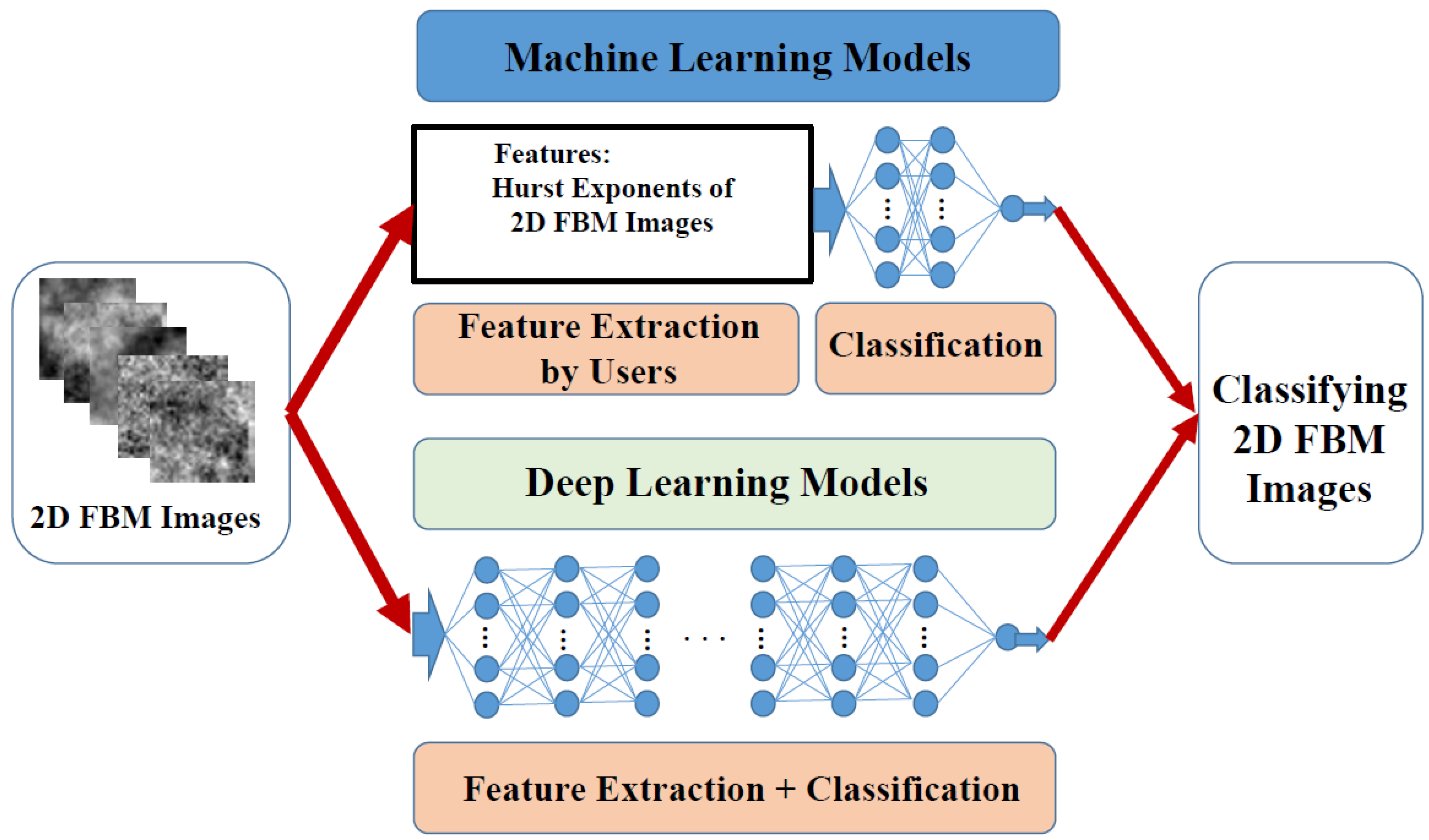
In the paper, we investigate the resolution of the Hurst exponent through machine learning and deep learning. For machine learning, we first estimate two kinds of data of Hurst exponents—fractional Brownian surfaces (FBSs; true data) and 2D FBM images (surfaces saved as images, thereby losing some details) or simply called fractional Brownian images (FBIs), and then classify these numeric estimates by four machine learning models. For deep learning, we directly classify these images by four deep learning models without feature selection and extraction performed by users.

3.1. Experimental Settings

To understand the effectiveness, we considered two groups of Hurst exponents or two kinds of classes—one has 11 Hurst exponents (11 classes) and the other 21 Hurst exponents (21 classes). The 11 Hurst exponents are composed of H = 1/22, 3/22, …, and 21/22; the 21 Hurst exponents are composed of H = 1/42, 3/42, …, and 41/42. Hence, the resolution of 11 classes is 1/11, and the resolution of 21 classes is 1/21.

Similar to Hoefer et al. [30], as our dataset, we generated 1000 realizations of 2D FBM of size 32 × 32 × 1 for each Hurst exponent or class and saved them as numerical data (called FBSs) as well as images (called 2D FBM images or FBIs). The procedure for each 2D FBM was as follows: First, we calculated the covariance matrix according to (4), which is related to (2). Second, we used the Cholesky factorization to decompose the covariance matrix in order to the lower triangular. Third, we generated a realization of white Gaussian noise with zero mean and unit variance. Finally, we generated a realization of 2D FBM by multiplying the lower triangular and the white noise. Hence, we generated 11,000 surfaces and images for 11 Hurst exponents and 21,000 surfaces and images for 21 Hurst exponents. Note that FBIs are approximate to FBSs with some details or information lost.

To understand some possible appearances of different Hurst exponents, Figure 3 shows three images, each with 16 patches of FBIs of size 32 × 32 × 1 generated from H = 1/22, H = 3/22, and H = 5/22; Figure 4 shows three images, each with 16 patches of FBIs of size 32 × 32 × 1 generated from H = 7/22, H = 9/22, and H = 11/22; Figure 5 shows three images, each with 16 patches of FBIs of size 32 × 32 × 1 generated from H = 13/22, H = 15/22, and H = 17/22; Figure 6 shows two images, each with 16 patches of FBIs of size 32 × 32 × 1 generated from H = 19/22 and H = 21/22.

From Figure 3, Figure 4, Figure 5 and Figure 6 (the images based on 11 Hurst exponents with resolution 1/11), we can obviously find that images of two neighboring Hurst exponents or classes are not easy to differentiate from each other by human beings, even for images of three neighboring Hurst exponents. Therefore, it can be easily understood that the images based on 21 Hurst exponents with resolution 1/21 are more difficult to classify from two to four neighboring Hurst exponents, especially for higher Hurst exponents.

3.2. Results and Discussion of Machine Learning Models

For four machine learning models, we experimented with five-fold cross-validation on the same estimates from the MLE for 2D FBM.

Table 1. The classification rates of four machine learning models on the estimates of FBSs of 11 Hurst exponents.

Models	Mean	Std.
LR	0.837	0.023
SVMs	0.839	0.023
KNNs	0.813	0.026
DT	0.826	0.025

shows the classification rate of four machine learning models that learned from the first numerical data—the estimates of the Hurst exponent from the MLE for FBSs of 11 Hurst exponents;

Table 2. The classification rates of four machine learning models on the estimates of FBIs of 11 Hurst exponents.

Models	Mean	Std.
LR	0.809	0.024
SVMs	0.814	0.023
KNNs	0.783	0.020
DT	0.800	0.023

shows the classification rate of four machine learning models that learned from the second numerical data—the estimates of the Hurst exponent from the MLE for FBIs of 11 Hurst exponents;

Table 3. The classification rates of four machine learning models on the estimates of FBSs of 21 Hurst exponents.

Models	Mean	Std.
LR	0.554	0.032
SVMs	0.560	0.033
KNNs	0.497	0.017
DT	0.496	0.021

shows the classification rate of four machine learning models that learned from the third numerical data—the estimates of the Hurst exponent from the MLE for FBSs of 21 Hurst exponents;

Table 4. The classification rates of four machine learning models on the estimates of FBIs of 21 Hurst exponents.

Models	Mean	Std.
LR	0.521	0.029
SVMs	0.532	0.031
KNNs	0.474	0.020
DT	0.475	0.020

shows the classification rate of four machine learning models that learned from the fourth numerical data—the estimates of the Hurst exponent from the MLE for FBIs of 21 Hurst exponents.

Among four machine learning models, we find from Table 1, Table 2, Table 3 and Table 4 that the SVM has the best classification rate of 0.839. Therefore, we chose the SVM as our compared subject to deep learning models. In line with our intuition, the classification rates based on the FBSs are better than those based on the FBIs because FBIs are saved as images from FBSs with some finer details lost.

Under the resolution of 1/11 of Hurst exponents, the classification rates are higher than 0.8 and acceptable; however, the classification rates are lower than 0.6 and generally unacceptable under the resolution of 1/21 of Hurst exponents.

For most situations, images are usually captured or acquired, and hence, for comparison with deep learning models that often use images as inputs, we run the SVM on the estimates of the Hurst exponent from the MLE for FBIs and produced the confusion matrix (

Table 5. The confusion matrix of SVMs on the estimates of FBIs of 11 Hurst exponents.

TC a\PC b	1	2	3	4	5	6	7	8	9	10	11
1	200	0	0	0	0	0	0	0	0	0	0
2	1	192	7	0	0	0	0	0	0	0	0
3	0	5	185	10	0	0	0	0	0	0	0
4	0	0	12	178	10	0	0	0	0	0	0
5	0	0	0	23	159	18	0	0	0	0	0
6	0	0	0	0	19	159	22	0	0	0	0
7	0	0	0	0	0	24	155	21	0	0	0
8	0	0	0	0	0	0	19	151	30	0	0
9	0	0	0	0	0	0	0	35	140	25	0
10	0	0	0	0	0	0	0	0	33	132	35
11	0	0	0	0	0	0	0	0	7	59	134

^a True Class; ^b Predicted Class.

) and the classification report (

Table 6. The classification report of SVMs on the estimates of FBIs of 11 Hurst exponents.

Classes	Precision	Recall	F1-Score	Support
1	1.00	1.00	1.00	200
2	0.97	0.96	0.97	200
3	0.91	0.93	0.92	200
4	0.84	0.89	0.87	200
5	0.85	0.80	0.82	200
6	0.79	0.80	0.79	200
7	0.79	0.78	0.78	200
8	0.73	0.76	0.74	200
9	0.67	0.70	0.68	200
10	0.61	0.66	0.63	200
11	0.79	0.67	0.73	200

). In the experiment, the SVM model used default parameters and was run under 80% data as the training set and 20% data as the test set.

Table 5 and Table 6 display a trend that lower Hurst exponents are easier to differentiate because they are much rougher to contain more details and much information; however, the worst case happens at Class 10 (H = 20/22) instead of the last class, Class 11 (H = 21/22) because the last class is not affected by its right neighboring Hurst exponent. Obviously, the best case is Class 1 (H = 1/22); its recall rate is 1, and its precision is almost 1.

3.3. Results and Discussion of Deep Learning Models

The MLE, as we know, is the best estimator for 2D FBM—it is an unbiased estimator and has the lowest mean-squared error. Even so, when its estimates are used to differentiate between the classes of the Hurst exponent or fractal dimension, the classification rate of the SVM classifier on these estimates is only 83.9% for FBSs and 81.4% for FBIs under the resolution of 1/11, and only 56.0% for FBSs and 53.2% for FBIs under the resolution of 1/21.

For images of size 32 × 32 × 1, the resolution is not very high, especially under the resolution of 1/21. Therefore, the first purpose of the paper is to investigate whether or not we can design a simple sequential network to achieve a higher classification rate, as well as whether some pretrained deep learning models can obtain higher classification rates. If so, the second purpose is to use these deep learning models to replace the role of the MLE for 2D FBM in order to efficiently and effectively recognize the classes of images—or equivalently estimate the Hurst exponent or its corresponding fractal dimension of images.

First, we designed a simple sequential network model and chose three pretrained models—AlexNet, GoogleNet, and Xception—as our compared subjects. Except for the AlexNet model, each model contains two types of modalities: one uses the size of the original images—32 × 32 × 1—as the size of the input layer, and hence no augmented operation is necessary; the other uses the size of the original model—for example, 227 × 227 × 3 for the AlexNet model—as the size of the input layer, and hence an augmented operation is needed. We call the first modality Type 1 and the second Type 2 and simply express them as AlexNet 1 and AlexNet 2, GoogleNet 1 and GoogleNet 2, as well as Xception1 and Xception 2.

Since the AlexNet model contains three pooling layers, making the size smaller and smaller, AlexNet 1 was not suitable for the size of our images. Therefore, the following four tables will not list their corresponding results. Totally, six models were considered and performed. All six models were run on the same FBIs or 2D FBM images and under five-fold cross-validation. The size of our images is 32 × 32 × 1.

In the case of Type 1, since our image size is different from those of the three pretrained models—227 × 227 × 3 for the AlexNet model (25 layers), 224 × 224 × 3 for the GoogleNet model (144 layers), and 299 × 299 × 3 for the Xception model (170 layers)—and the number of the output classes (11 or 21) is different from 1000 for three models, we adjusted the input layer, fully connected layer, and an output layer of the three pretrained models in order to run these models correctly. For convenience, when we refer to these adjusted models, we call them the adjusted AlexNet model, the adjusted GoogleNet model, and the adjusted Xception model, respectively, or simply AlexNet 1, GoogleNet 1, and Xception 1, respectively.

In the case of Type 2, we used an augmenter to make the image size (32 × 32 × 1) match the sizes (227 × 227 × 3, 224 × 224 × 3, or 299 × 299 × 3) of three pretrained models, and modified the corresponding fully-connected layer and output layer to meet the number of our classes, 11 or 21. We simply call them AlexNet 2, GoogleNet 2, and Xception 2, respectively. The augmenter was introduced only for resizing the original images to the corresponding sizes of three pretrained models.

For a fair comparison, all six models were performed in the same computing environment. (1) Hardware: a computer of Intel^® Xeon(R) W-2235 CPU @ 3.80 GHz with 48.0 GB RAM (47.7 GB available), together with a GPU processor (NVIDIA RTX A4000); (2) operating system: Windows 11 Professional Workstation, version 21 H2; (3) programming software: MATLAB R2022a; (4) training options: the solver was stochastic gradient descent with momentum (SGDM); the mini-batch size was 128; the initial learning rate was 0.001; the learning rate schedule was piecewise; the learning rate drop factor was 0.1; the learning rate drop period was 20; the shuffle was for every epoch; the validation frequency was 30; the number of epochs was 30; and the other options were set to default.

Since the mini-batch size was 128 and five-fold was performed, the number of iterations per epoch was 68 (11,000 × 0.8/128 = 68.75) for 11 Hurst exponents, 2040 iterations in total; the number of iterations per epoch was 131 (21,000 × 0.8/128 = 131.25) for 21 Hurst exponents, 3930 iterations in total.

Our proposed model is a 29-layer sequential network composed of an image input layer, five groups of a convolutional layer, a batch normalization layer, a ReLU layer, and a maximum pooling layer (in total, 20 layers), one group of a convolutional layer, a batch normalization layer, and a ReLU layer (in total, three layers), one group of a fully connected layer and a ReLU layer (in total, two layers), as well as the final group of a fully connected layer, a softmax layer, and a classification layer (in total, three layers).

According to the structures and characteristics of our FBIs, we adopted a simple design concept for our proposed model; that is, the filters were regularly configured, and their corresponding sizes were increased. Therefore, our proposed model was arranged as follows. The image input layer is of size 32 × 32 × 1; the first convolutional layer contains 128 filters of size 3 × 3; the second convolutional layer contains 128 filters of size 5 × 5; the third convolutional layer contains 128 filters of size 7 × 7; the fourth convolutional layer contains 128 filters of size 9 × 9; the fifth convolutional layer contains 128 filters of size 11 × 11; the sixth convolutional layer contains 128 filters of size 13 × 13. All maximum pooling layers are of size 2 × 2 with stride two. The output size of the first fully connected layer is 10 times 11 or 21 (110 or 210); the output size of the second fully connected layer is 11 or 21, depending on the number of classes. For clarity,

Table 7. The number of layers for our proposed model.

Group of Layers	Number of Layers per Group	Number of Groups	Number of Layers	Sizes or Number of Filters (Sizes of Convolutional Layers)
an image input layer	1	1	1	32 × 32 × 1
a convolutional layer + a batch normalization layer + a ReLU layer + a maximum pooling layer (2 × 2) (2)	4	5	20	128 (3 × 3) + 128(5 × 5) + 128 (7 × 7) + 128 (9 × 9) + 128 (11 × 11)
a convolutional layer + a batch normalization layer + a ReLU layer	3	1	3	128 (13 × 13)
a fully connected layer + a ReLU layer	2	1	2	10 times 11 or 21 (Output size of a fully connected layer)
a fully connected layer + a softmax layer + a classification layer	3	1	3	11 or 21 (Output size of a fully connected layer)

shows the architecture of our proposed model.

In the case of 11 classes,

Table 8. The mean and standard deviation of classification rates of four deep learning models for 11 classes.

Models	Mean	Std.
Our model	0.9600	0.0056
AlexNet 2	0.8943	0.0101
GoogleNet 1	0.9324	0.0026
GoogleNet 2	0.9085	0.0091
Xception 1	0.6551	0.0180
Xception 2	0.8940	0.0092

shows that our proposed model has the best accuracy at 0.9600, and its corresponding standard deviation is 0.0056; the second best is GoogleNet 1, with an accuracy of 0.9324 and the smallest standard deviation of 0.0026. The worst model for our FBIs is Xception 1, with an accuracy of 0.6551 and the largest standard deviation of 0.0180.

In the case of 21 classes,

Table 9. The mean and standard deviation of classification rates of four deep learning models for 21 classes.

Models	Mean	Std.
Our model	0.9370	0.0063
AlexNet 2	0.8358	0.0109
GoogleNet 1	0.9266	0.0046
GoogleNet 2	0.8515	0.0142
Xception 1	0.6410	0.0498
Xception 2	0.8918	0.0127

shows that our proposed model also has the best accuracy at 0.9370 and its corresponding standard deviation is 0.0063; the second best is also GoogleNet 1 with an accuracy of 0.9266 and the smallest standard deviation at 0.0046. The worst model for our FBIs is also Xception 1, with an accuracy of 0.6410 and the largest standard deviation at 0.0498. Similar to machine learning models, it is expected that the case of 21 classes is generally worse than the case of 11 classes.

Based on the same FBIs, five deep learning models (except for Xception 1) on 11 classes are better than the best accuracy of 0.814 (SVMs) from four machine learning models, where the only feature of the estimated Hurst exponents was considered. In the other case of 21 classes, six deep learning models are all better than the best accuracy of 0.56 (SVMs) from four machine learning models.

When training time is important, our proposed model is also the first choice.

Table 10. The training time (in minutes) and the ratio of four deep learning models for 11 classes.

Models	Time	Ratio
Our model	1.31	1.00
AlexNet 2	12.71	9.66
GoogleNet 1	3.99	3.04
GoogleNet 2	19.62	14.92
Xception 1	11.78	8.96
Xception 2	664.21	505.13

and

Table 11. The training time (in minutes) and the ratio of four deep learning models for 21 classes.

Models	Time	Ratio
Our model	2.73	1.00
AlexNet 2	29.39	10.78
GoogleNet 1	8.10	2.97
GoogleNet 2	42.36	15.53
Xception 1	24.47	8.98
Xception 2	1352.69	496.13

shows that the training times of 11 classes and 21 classes are 1.41 and 2.71 min, respectively. In addition, these two tables also show the time ratios of other models to our model. The second efficient model is GoogleNet 1, with 4.15 and 8.54 min for 11 classes and 21 classes. The worst efficient model is Xception 2 with 664.21 and 1352.69 min for 11 classes and 21 classes.

To further analyze the distribution of the incorrectly classified classes, we show two promising models—our proposed model and GoogleNet 1—for discussion. For our proposed model, we list the confusion matrix of the first fold of five-fold cross-validation for 11 classes in Figure 7 and the complete confusion matrix and its lower right part for clarity for 21 classes in Figure 8a,b (when zoomed in, the figure will be easy to read). The diagonal cells show the number of cases that were correctly classified, and the off-diagonal cells show the misclassified cases.

Similar to Table 5 for SVMs, the worst sensitivity or recall (79.5%) among 11 classes occur in the last but one class, Class 10, and the worst precision (84.1%) also occurs in the last but one class. Therefore, the worst classification rate also occurs in the last but one class. Relatively, lower Hurst exponents or rougher images are easier to differentiate; the boundary lies in the middle class, Class 6 (H = 1/2).

The worst sensitivity or recall (49.0%) among 21 classes occurs in the last to one class, Class 20; likewise, the worst precision (58.3%) also occurs in the last but one class; therefore, the worst classification rate also occurs in the last but one class. Relatively, higher Hurst exponents or smoother images are more difficult to differentiate because their hidden features get lesser. The boundary lies about in the middle class, Class 11; that is, the classes of Hurst exponents lower than 0.5 can be correctly classified. Generally, the classification rate gets lower as the Hurst exponent gets larger.

As a comparison, we also list the confusion matrix of the first fold of the five-fold cross-validation of GoogleNet 1 for 11 classes in Figure 9 and the complete confusion matrix and its lower right part for clarity for 21 classes in Figure 10a,b (when zoomed in, the figure will be easy to read).

The worst sensitivity or recall (74.0%) among 11 classes occur in the last but one class, Class 10; likewise, the worst precision (76.7%) also occurs in the last but one class; therefore, the worst classification rate occurs in the last but one class. Likewise, lower Hurst exponents or rougher images are easier to differentiate; the diagonal cells show smaller numbers as the Hurst exponent gets larger.

The worst sensitivity or recall (55.0%) among 21 classes occur in the last but one class, Class 20; likewise, the worst precision (57.0%) also occurs in the last but one class; therefore, the worst classification occurs in the last but one class. Similarly, higher Hurst exponents or smoother images are more difficult to differentiate. In general, the classification rate gets lower as the Hurst exponent increases.

3.4. Comprehensive Discussion

Traditionally, when we want to estimate the fractal dimensions of images, we use an estimator to compute. If necessary, we also can further use the fractal dimensions to classify their classes or types. In the past, the box-counting method was often used to estimate because of its simplicity; however, its accuracy is considerably low, and hence it is often unreliable, thereby resulting in a low recognition rate.

Recently, Chang [22] proposed an efficient MLE for 2D FBM, which is the most accurate estimator and, so far, the most efficient estimator among the MLEs. However, its computational time is still high for applications with larger image sizes and/or database sizes, and hence it is not appropriate for tasks of quick evaluation and analysis, especially for real-time systems.

Therefore, when we want to get the feature map of an original image by transforming the sub-images of the image to a matrix with the corresponding Hurst exponent as an entry or element, it is essential to find out an alternative estimation tool for a wide range of use. This is the second purpose of the paper.

In the paper, we have experimentally confirmed in the images of size 32 × 32 × 1 that the classification rates of suitably designed or chosen deep learning models can outperform those of machine learning models that receive the only feature—the estimated Hurst exponents from the efficient MLE. The computational cost of machine learning models can be neglected, but taking the only feature is terribly high.

In general, directly estimating the Hurst exponent of images is enough to analyze the differences between images; the classification is practically not necessary. Performed on the estimated Hurst exponents, machine learning models aim to compare with deep learning models as well as to further evaluate the benefits of deep learning models. If workable, we can use well-trained deep learning models to replace the role of the efficient MLE as estimation or further feature transformation.

At present, the comparison may not be considered fair because we use only one indicator as our feature for machine learning models, but deep learning models can implicitly and automatically extract or capture as more and more features as possible. However, the comparison tells us that deep learning models do work well even for the 2D FBM images from a 2D random process—various appearances coming from different realizations with the same parameter, as shown in Figure 3, Figure 4, Figure 5 and Figure 6. In the future, we can manually select other promising indicators as our features, for example, entropy and spectrum, to raise the classification rate.

Surprisingly, the chosen three pretrained networks—AlexNet, GoogleNet, and Xception—also work well for 2D FBM images (or FBIs) of size 32 × 32 × 1; in addition, the adjusted GoogleNet model is better than the adjusted AlexNet model and the adjusted Xception model in terms of the computational cost and classification rate.

These pretrained networks, as we know, were designed for 1000 common object categories, such as keyboard, mouse, pencil, and many animals. They did not see the hidden features of FBIs and were not trained with them, and hence, intuitively, they should not perform well. However, they not only work better than machine learning models with the only feature of the estimated Hurst exponents, but they also give us a promising prospect for the future, especially GoogleNet 1. As for other image sizes, further experiments are needed in order to find out the most suitable deep-learning model for different cases or situations.

In the experiments, we find that the models of Type 1—with the original images as the input images—can work better than machine learning models with the best estimates of the Hurst exponent as the only feature except Xception 1. Xception 1 cannot work well for a small image size. It is reasonable because Xception 1 cannot capture enough features for its large input size of 299 × 299 × 3 and its high layer number of 170. For the models of Type 2—with resizing the original images as the input images, they give similar results and are all better than machine learning models with the best estimates of the Hurst exponent as the only feature. However, the computational cost of model Type 2 is much higher than that of its corresponding model Type 1 because model Type 2 needs resizing and always performs on larger images.

The success of the pretrained models illustrates that 2D FBM images, even being random characteristics, can still be learned from concrete lines and/or curves to abstract patterns through low-level to high-level layers.

With the success of pretrained networks, on the other hand, we establish a regular structure of network layers according to the characteristics of 2D FBM images. It turns out that our proposed simple sequential deep learning model does work well for 11 and 21 classes under the images of size 32 × 32 × 1. In addition, our proposed model is the best in terms of the classification rate and computational cost. GoogleNet 1 is the second.

For further applications to the estimation of the Hurst exponent, we also want to know whether these promising deep learning models are still equivalently better than the MLE in terms of the mean absolute error (MAE) and mean square error (MSE) as ordinal classification metrics, especially as numerical ordinal classification metrics like our dataset.

Since our dataset is balanced and was stratified for the five-fold cross-validation, as well as all classes are equally spaced, each corresponding to a number, we simply chose the general, not weighted, MAE and MSE as our comparison metrics.

Table 12. Comparison among four methods in terms of the MAE and MSE.

		MAE		MSE
Methods	No. of Classes	Mean	Std.	Mean	Std.
Our model	11	3.64 × 10−3	5.02 × 10−4	3.33 × 10−4	4.47 × 10−5
	21	3.22 × 10−3	3.42 × 10−4	1.74 × 10−4	2.15 × 10−5
GoogleNet 1	11	6.16 × 10−3	2.55 × 10−4	5.61 × 10−4	2.60 × 10−5
	21	3.68 × 10−3	1.91 × 10−4	1.93 × 10−4	7.81 × 10−6
MLE (FBSs)	11	2.60 × 10−2	2.05 × 10−2	1.09 × 10−3	1.68 × 10−3
	21	2.59 × 10−2	2.05 × 10−2	1.09 × 10−3	1.69 × 10−3
MLE (FBIs)	11	2.83 × 10−2	2.45 × 10−2	1.40 × 10−3	2.73 × 10−3
	21	2.93 × 10−2	2.83 × 10−2	1.66 × 10−3	4.46 × 10−3

shows the comparison among four methods—the MLE was estimated on two datasets (FBSs and FBIs)—in terms of the MAE and MSE.

It is obvious from Table 12 that our model is also the best and the second is GoogleNet 1 in terms of the MAE and MSE. In addition, the results of 21 classes are better than those of 11 classes for our model and GoogleNet 1. Therefore, we choose our proposed model and GoogleNet 1 with 21 classes as tools for estimation or feature transformation and further compare both models with the efficient MLE in the following Applications section.

4. Applications

For medical images, there often appear some fractal characteristics—especially in the small regions—and hence if we want to recognize the differences between tissues, in the past, we only used estimators to compute their fractal dimensions or their corresponding Hurst exponents, and then judged them by their estimates. Under the images of size 32 × 32 × 1, experimental results show that some pretrained or well-designed deep learning models can “equivalently” outperform the efficient MLE—the best estimator—in an efficient and effective way; therefore, in the future, we can adopt some promising deep learning models to classify—or equivalently estimate—the Hurst exponent.

For comparison, we chose one medical image database—the chest X-ray database—from Kaggle [40]; they are grayscale images. First, we find out the smallest size of all images—127 × 384—as our input size. According to the size, we then clipped the central parts of all images because other parts generally contain some unimportant and unrelated components. Finally, we chose one clipped image as our subject, shown in Figure 11.

Among experimental models, our proposed model and GoogleNet 1 run on 21 classes suitably serve the role of transforming the original image to two feature maps of the Hurst exponent. For estimation or feature transformation, we first chose the size of each sub-image as 32 × 32—the size of our model design. Second, we chose 1 as our stride or shift in the horizontal and vertical directions. For all sub-images, on the one hand, we classified them through our proposed model and GoogleNet 1 and then converted these classes to their corresponding Hurst exponents—for example, the first class is equivalent to H = 1/42 and the last (or 21st) class equivalent to H = 41/42. On the other hand, we estimated them through the efficient MLE. Figure 12 shows their resultant images or feature maps (96 × 353) (top) and their corresponding negatives (bottom). The darker points correspond to the smaller Hurst exponents; the lighter points, the larger Hurst exponents. The black point is equivalent to H = 0, and the white point is equivalent to H = 1.

It is obvious from Figure 12 that these three sets of feature maps are different from one another because all sub-images are not exactly images from 2D FBM, but they are just modeled as 2D FBM. Different deep learning models, as we know, generally learn and extract various hidden features from different perspectives. For exact images from 2D FBM, they eventually can organize all learned parameters well into the correct classes. However, when the sub-images are not exactly images from 2D FBM, the final results may be different from one another, except that different models have similar learning structures.

Even though the three methods—two deep learning models and one estimator—give different appearances or explanations for the same image, they all follow their own unique rules to classify or estimate the Hurst exponent based on the learned parameters, and hence, each will give its own consistent interpretation.

Therefore, in terms of feature maps, the different appearances should be a good thing because real-world images are often not perfect for their claimed model, such as 2D FBM. We can extract diverse features from various perspectives through different models, and then we will fuse these features together for better analysis.

Figure 12 shows that we can extract diverse features from different trained learning models, and these feature maps are simpler in structure than their original image. That is the essence of feature engineering [29]: making a problem easier by expressing it in a simpler way. For effectiveness, feature engineering usually requires understanding the problem in depth [29]. That is why we choose to learn the Hurst exponent—or equivalently, the fractal dimension—features from 2D FBM because it is considered suitable for describing the characteristics of medical images and natural scenes.

As a tool of feature engineering, the trained deep learning models on the Hurst exponent of 2D FBM are effective. Furthermore, we would like to know whether they are efficient because the MLE has already been available for the role of feature engineering.

Table 13. Classifying or estimating time (in seconds) and its ratio.

Models	Mean	Ratio
Our model	0.0034	1.00
GoogleNet 1	0.0138	4.09
MLE	0.4996	148.36

lists the computational times of three methods. Obviously, our proposed model is the smallest—classifying each sub-image only spends 0.0034 s, the second is GoogleNet 1, and the largest is the efficient MLE with a ratio of 148.36 to our proposed model. Therefore, our proposed model is suitable for estimation or feature transformation for larger databases and/or larger image sizes. GoogleNet 1 is also suitable. Therefore, it is considered meaningful to implement the idea of classifying 2D FBM images through deep learning as a tool of feature engineering for replacing the role of the MLE.

With the success of effectively and efficiently classifying 2D FBM images through deep learning, we can make more use of these trained deep learning models for an automatic tool as feature engineering. Therefore, in the future, we will try hard to find out other more suitable deep learning models, and then, we can use these diverse models to extract various features. With these diverse sources of feature information, we can further design some multiple-input and/or multiple-stream deep learning models to recognize complicated images in order to obtain a higher classification rate than a single-input model with the original images as input.

5. Conclusions

Recently, an efficient MLE for 2D FBM has been proposed to estimate Hurst exponents or their corresponding fractal dimensions of fractal surfaces or images. The MLE for 2D FBM is an unbiased estimator and the best in mean-squared error, but it is inevitable to contain estimation error. That is, the exact value of any estimated Hurst exponent is not absolutely reliable. Accordingly, in the paper, we replace estimated Hurst exponents with the corresponding Hurst exponents of their classes or equivalent Hurst exponents. For the Hurst exponent, three ranges or cases are meaningful: H < 0.5, H = 0.5, and H > 0.5, and different values tell different levels of seriousness. The exact H = 0.5, however, cannot be evaluated. Therefore, we considered two cases of 11 classes and 21 classes of the Hurst exponent to contain the three ranges mentioned above.

Experimental results show that the best classification rate of 11 classes through four machine learning models run on the estimated Hurst exponents is 81.4%; that of 21 classes is 53.2%. Therefore, the exact value of any estimated Hurst exponent has lost its true meaning under the resolution of 1/21. On the other hand, when deep learning models were run on the same images, the best classification rate of 11 classes through three deep learning models was 96.00%; that of 21 classes was 93.70%.

Since deep learning models, if well designed or chosen, can learn more from various hidden features, the results of deep learning models are better than those of machine learning models learning from the only feature—the estimated Hurst exponents. In the future, except for the estimated Hurst exponents, we would like to find out other useful features to raise the classification rate of machine learning models and further compare the results to those of deep learning models by further adjusting or choosing hyperparameters. With the success of deep learning models, more inputs will also be developed to improve the whole performance in the upcoming future.

Based on their high classification accuracies, these well-designed or well-chosen pretrained deep learning models can be used to “equivalently” estimate the Hurst exponent or fractal dimension—first, determine the class of an image and then calculate its corresponding Hurst exponent. Consequently, the time saving can be up to 148 times that of the best estimator—the MLE. In addition, different models will learn various hidden features; hence, when they are applied to “equivalently” estimate the Hurst exponents of practical images—modeled as 2D FBM, but not the exact one, they can find out various appearances that contribute to explaining diverse details from various perspectives.

More importantly, the concept of feature maps—in our case, transforming an original image to a feature map of the Hurst exponent—can be widely used to develop other feature maps, such as spectrum or entropy maps, in order to raise the whole recognition rate.

References

1. Huang, P.-W.; Lee, C.-H. Automatic classification for pathological prostate images based on fractal analysis. IEEE Trans. Med. Imaging 2009, 28, 1037–1050. [Google Scholar] [CrossRef] [PubMed]
2. Lin, P.-L.; Huang, P.-W.; Lee, C.-H.; Wu, M.-T. Automatic classification for solitary pulmonary nodule in CT image by fractal analysis based on fractional Brownian motion model. Pattern Recognit. 2013, 46, 3279–3287. [Google Scholar] [CrossRef]
3. He, D.; Liu, C. An online detection method for coal dry screening based on image processing and fractal analysis. Appl. Sci. 2022, 12, 6463. [Google Scholar] [CrossRef]
4. Yakovlev, G.; Polyanskikh, I.; Belykh, V.; Stepanov, V.; Smirnova, O. Evaluation of changes in structure of modified cement composite using fractal analysis. Appl. Sci. 2021, 11, 4139. [Google Scholar] [CrossRef]
5. Di Crescenzo, A.; Martinucci, B.; Mustaro, V. A model based on fractional Brownian motion for temperature fluctuation in the Campi Flegrei Caldera. Fractal Fract. 2022, 6, 421. [Google Scholar] [CrossRef]
6. Hu, H.; Zhao, C.; Li, J.; Huang, Y. Stock prediction model based on mixed fractional Brownian motion and improved fractional-order particle swarm optimization algorithm. Fractal Fract. 2022, 6, 560. [Google Scholar] [CrossRef]
7. Falconer, K. Fractal Geometry: Mathematical Foundations and Applications; John Wiley & Sons: New York, NY, USA, 1990. [Google Scholar]
8. Barnsley, M.F.; Devaney, R.L.; Mandelbrot, B.B.; Peitgen, H.-O.; Saupe, D.; Voss, R.F. The Science of Fractal Images; Springer: New York, NY, USA, 1988. [Google Scholar]
9. Mandelbrot, B.B. The Fractal Geometry of Nature; W. H. Freeman and Company: New York, NY, USA, 1983. [Google Scholar]
10. Gonçalves, W.N.; Bruno, O.M. Combining fractal and deterministic walkers for texture analysis and classification. Pattern Recognit. 2013, 46, 2953–2968. [Google Scholar] [CrossRef]
11. Zuñiga, A.G.; Florindo, J.B.; Bruno, O.M. Gabor wavelets combined with volumetric fractal dimension applied to texture analysis. Pattern Recognit. Lett. 2014, 36, 135–143. [Google Scholar] [CrossRef] [Green Version]
12. Pentland, A.P. Fractal-based description of natural scenes. IEEE Trans. Pattern Anal. Mach. Intell. 1984, 6, 661–674. [Google Scholar] [CrossRef]
13. Chen, C.-C.; Daponte, J.S.; Fox, M.D. Fractal feature analysis and classification in medical imaging. IEEE Trans. Med. Imaging 1989, 8, 133–142. [Google Scholar] [CrossRef]
14. Gagnepain, J.J.; Roques-Carmes, C. Fractal approach to two-dimensional and three dimensional surface roughness. Wear 1986, 109, 119–126. [Google Scholar] [CrossRef]
15. Sarkar, N.; Chaudhuri, B.B. An efficient differential box-counting approach to compute fractal dimension of image. IEEE Trans. Syst. Man Cybern. 1994, 24, 115–120. [Google Scholar] [CrossRef] [Green Version]
16. Sarkar, N.; Chaudhuri, B.B. An efficient approach to estimate fractal dimension of textural images. Pattern Recognit. 1992, 25, 1035–1041. [Google Scholar] [CrossRef]
17. Chen, S.S.; Keller, J.M.; Crownover, R.M. On the calculation of fractal features from images. IEEE Trans. Pattern Anal. Mach. Intell. 1993, 15, 1087–1090. [Google Scholar] [CrossRef]
18. Jin, X.C.; Ong, S.H.; Jayasooriah. A practical method for estimating fractal dimension. Pattern Recognit. Lett. 1995, 16, 457–464. [Google Scholar] [CrossRef]
19. Bruce, E.N. Biomedical Signal Processing and Signal Modeling; John Wiley & Sons: New York, NY, USA, 2001. [Google Scholar]
20. Li, J.; Du, Q.; Sun, C. An improved box-counting method for image fractal dimension estimation. Pattern Recognit. 2009, 42, 2460–2469. [Google Scholar] [CrossRef]
21. Peleg, S.; Naor, J.; Hartley, R.; Avnir, D. Multiple resolution texture analysis and classification. IEEE Trans. Pattern Anal. Mach. Intell. 1984, 6, 518–523. [Google Scholar] [CrossRef] [PubMed] [Green Version]
22. Chang, Y.-C. An efficient maximum likelihood estimator for two-dimensional fractional Brownian motion. Fractals 2021, 29, 2150025. [Google Scholar] [CrossRef]
23. Russell, S.; Norvig, P. Artificial Intelligence: A Modern Approach, 4th ed.; Pearson Education Limited: Harlow, UK, 2021. [Google Scholar]
24. Lowndes, A.B. Deep Learning with GPUs: For the Beginner; LAP LAMBERT: London, UK, 2016. [Google Scholar]
25. Géron, A. Hands-On Machine Learning with Scikit-Learn and TensorFlow: Concepts, Tools, and Techniques to Build Intelligent Systems; O’Reilly: Sebastopol, CA, USA, 2017. [Google Scholar]
26. Raschka, S.; Mirjalili, V. Python Machine Learning: Machine Learning and Deep Learning with Python, Scikit-Learn, and TensorFlow 2, 3rd ed.; Packt: Birmingham, UK, 2019. [Google Scholar]
27. Beale, M.H.; Hagan, M.T.; Demuth, H.B. Deep Learning Toolbox: User’s Guide; MathWorks: Natick, MA, USA, 2022. [Google Scholar]
28. Rivas, P. Deep Learning for Beginner’s Guide to Getting Up and Running with Deep Learning from Scratch Using Python; Packt: Birmingham, UK, 2020. [Google Scholar]
29. Chollet, F. Deep Learning with Python; Manning: New York, NY, USA, 2018. [Google Scholar]
30. Hoefer, S.; Hannachi, H.; Pandit, M.; Kumaresan, R. Isotropic two-dimensional Fractional Brownian Motion and its application in Ultrasonic analysis. In Proceedings of the Engineering in Medicine and Biology Society, 14th Annual International Conference of the IEEE, Paris, France, 29 October–1 November 1992; pp. 1267–1269. [Google Scholar]
31. Balghonaim, A.S.; Keller, J.M. A maximum likelihood estimate for two-variable fractal surface. IEEE Trans. Image Process. 1998, 7, 1746–1753. [Google Scholar] [CrossRef] [Green Version]
32. McGaughey, D.R.; Aitken, G.J.M. Generating two-dimensional fractional Brownian motion using the fractional Gaussian process (FGp) algorithm. Phys. A 2002, 311, 369–380. [Google Scholar] [CrossRef]
33. Schilling, R.J.; Harris, S.L. Applied Numerical Methods for Engineers: Using MATLAB and C; Brooks/Cole: New York, NY, USA, 2000. [Google Scholar]
34. Chang, Y.-C. N-Dimension Golden Section Search: Its Variants and Limitations. In Proceedings of the 2nd International Conference on BioMedical Engineering and Informatics (BMEI2009), Tianjin, China, 17–19 October 2009. [Google Scholar]
35. Ballester, P.; Araujo, R.M. On the performance of GoogLeNet and AlexNet applied to sketches. In Proceedings of the AAAI Conference on Artificial Intelligence, Phoenix, AZ, USA, 12–17 February 2016; pp. 1124–1128. [Google Scholar]
36. Szegedy, C.; Liu, W.; Jia, Y.; Sermanet, P.; Reed, S.; Anguelov, D.; Erhan, D.; Vanhoucke, V.; Rabinovich, A. Going deeper with convolutions. arXiv 2014, arXiv:1409.4842. [Google Scholar]
37. Chollet, F. Xception: Deep learning with depthwise separable convolutions. In Proceedings of the 2017 IEEE Conference on Computer Vision and Pattern Recognition (CVPR), Honolulu, HI, USA, 21–26 July 2017; pp. 1800–1807. [Google Scholar]
38. Szymak, P.; Piskur, P.; Naus, K. The effectiveness of using a pretrained deep learning neural networks for object classification in underwater video. Remote Sens. 2020, 12, 3020. [Google Scholar] [CrossRef]
39. Maeda-Gutiérrez, V.; Galván-Tejada, C.E.; Zanella-Calzada, L.A.; Celaya-Padilla, J.M.; Galván-Tejada, J.I.; Gamboa-Rosales, H.; Luna-García, H.; Magallanes-Quintanar, R.; Méndez, C.A.G.; Olvera-Olvera, C.A. Comparison of convolutional neural network architectures for classification of tomato plant diseases. Appl. Sci. 2020, 10, 1245. [Google Scholar] [CrossRef]
40. Chest X-ray Images (Pneumonia). Available online: https://www.kaggle.com/paultimothymooney/chest-xray-pneumonia (accessed on 24 September 2021).
Figure 1. The two adopted procedures for classifying 2D FBM images based on the same 2D FBM images.
Applsci 13 00803 g001
Figure 2. The procedure for transfer learning of pretrained models.
Applsci 13 00803 g002
Figure 3. Three images, each with 16 patches from different realizations of H = 1/22 (a) and H = 3/22 (b), and H = 5/22 (c).
Applsci 13 00803 g003
Figure 4. Three images, each with 16 patches from different realizations of H = 7/22 (a) and H = 9/22 (b), and H = 11/22 (c).
Applsci 13 00803 g004
Figure 5. Three images, each with 16 patches from different realizations of H = 13/22 (a) and H = 15/22 (b), and H = 17/22 (c).
Applsci 13 00803 g005
Figure 6. Two images, each with 16 patches from different realizations of H = 19/22 (a) and H = 21/22 (b).
Applsci 13 00803 g006
Figure 7. The confusion matrix of the first fold of the five-fold cross-validation of our proposed model for 11 classes.
Applsci 13 00803 g007
Figure 8. The complete confusion matrix (a) and its lower right part (b) for clarity of the first fold of the five-fold cross-validation of our proposed model for 21 classes.
Applsci 13 00803 g008
Figure 9. The confusion matrix of the first fold of the five-fold cross-validation of GoogleNet 1 for 11 classes.
Applsci 13 00803 g009
Figure 10. The complete confusion matrix (a) and its lower right part (b) for clarity of the first fold of the five-fold cross-validation of GoogleNet 1 for 21 classes.
Applsci 13 00803 g010
Figure 11. A sample of clipped chest X-ray images (127 × 384).
Applsci 13 00803 g011
Figure 12. The feature image or map (96 × 353) (top) and its corresponding negative (bottom) of transforming a clipped chest X-ray image (127 × 384) to Hurst exponents through our proposed model (a), GoogleNet 1 (b), and MLE (c).
Applsci 13 00803 g012aApplsci 13 00803 g012b