Article

Stiffening Cello Bridges with Design

Musical Acoustics Lab at the Violin Museum of Cremona, DEIB, Politecnico di Milano, Cremona Campus, 26100 Cremona, Italy
*
Author to whom correspondence should be addressed.
Appl. Sci. 2023, 13(2), 928; https://doi.org/10.3390/app13020928
Submission received: 7 December 2022 / Revised: 4 January 2023 / Accepted: 5 January 2023 / Published: 10 January 2023
(This article belongs to the Special Issue Mechanics, Dynamics and Acoustics of Musical Instruments)

Abstract

:
In instruments of the violin family, the bridge is the part in charge of transferring the vibrational energy of the strings into the body and therefore contributes greatly to the sound of the instrument. The bridge needs to be light enough to efficiently transmit the strings’ movement yet rigid enough to support the static load of the strings. Historically, there have been several attempts at solving this problem with different designs, arriving in the early 1800s at the two current models: the French and the Belgian. Recently, in Cremona, Italy, the Amorim family of luthiers has developed a new cello bridge design. Inspired by their work, we study the influence of the shape of the legs of the cello bridge on its static and vibrational behavior through parametric modeling and simulations using the Finite Element Method. In particular, we perform displacement and modal analysis for different boundary conditions, providing in addition a detailed description of the mode shapes. We also compute and compare Frequency Response Functions for the different geometries. Our results show that shape can indeed be used to control the vibrational and static responses of the cello and consequently tune its sound.

1. Introduction

The modern cello bridge’s design has remained pretty much intact since its introduction in the late 1700s [1]. The upper shape of the bridge is determined by playability—the musician needs to be able to bow in each of the strings—whereas the lower part needs to perfectly match the belly of the instrument. The middle part, however, has seen the most variation in design during its history. One wants a bridge that is light enough to transfer as much energy as possible to the body of the instrument, yet strong enough to support the load of the strings without breaking or deforming [2,3].
Bridges commonly used nowadays fall into the “French” or the “Belgian” model, the former being shorter and wider, while the latter is more slender and has longer legs. It is known by makers that different designs favor different sounds, yet there is no clear scientific understanding of this phenomenon. Recently, the Cremonese luthier Luiz Amorim started designing and using a revised version of the bridge in which the legs, rather than being curved, are carved straight from the center of the bridge towards the instrument. Pictures of a traditional bridge and Amorim’s cello bridge are shown in Figure 1.
Only a small portion of the literature in musical acoustics focus specifically on the cello bridge. The most relevant and complete review of the behavior of bridges is given by Fletcher and Rossings in [2] and by Rossings in [3]. Most of their discussion considers violin bridges and is extended to cello bridges only partially. In all instruments of the violin family, the bridge serves two main purposes. It statically sustains the strings, holding them in place at the correct height and at the correct distance from the fingerboard, effectively determining their vibrating length and guaranteeing the possibility for the player to bow each string individually. Moreover, the bridge also acts as very necessary impedance adapter between the strings and the body, and transforms the mainly lateral motion of the firsts into mainly vertical forces on the top. This filter can be controlled by the addition of mass or the stiffening of the bridge [4].
Inspired by the design modifications of the Amorim family, we study the relationship between the shape of the legs in a cello bridge and its mechanical properties: dynamic as well as static. By parameterizing the shape variation, we can easily study how the design determines the vibrational response of the bridge. This relationship between shape and vibrational behavior has been greatly studied in the case of the violin and the guitar [5,6,7] but has not yet been applied to the cello. In this article, we aim to set that record straight.

2. Materials and Methods

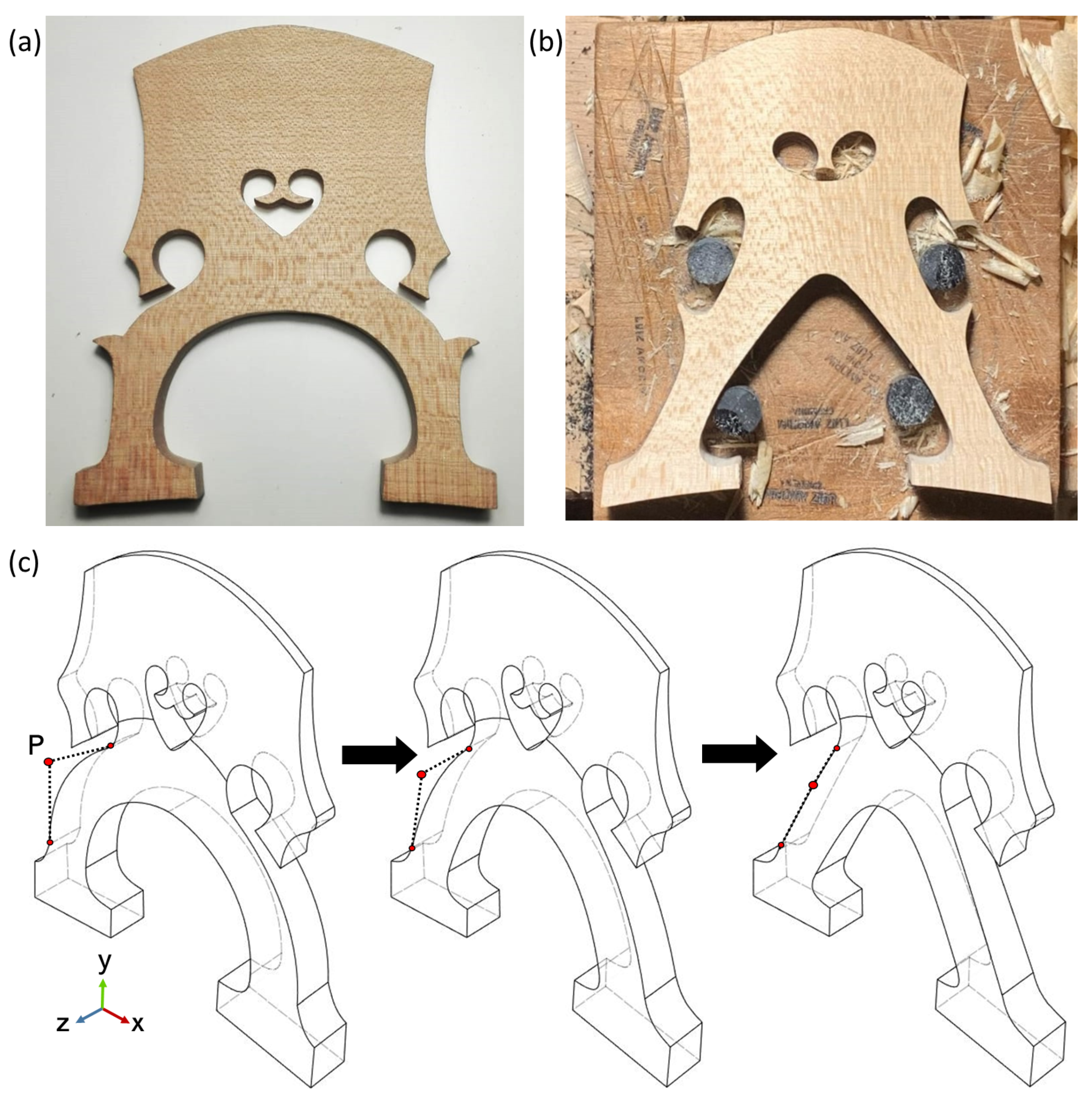
2.1. Modeling of the Bridge

In the study, we considered a parametric interpolation between two different models: on the one hand is a traditional French model, and on the other hand, the bridge design proposed by the Amorim family, referred to as “Model X” (Figure 1b). The 3D geometry of the bridges has been modeled through the CAD software Fusion 360.
The terminology used in the description of the bridge can be found in Figure A1. To build the Normal Model, we drew the outline of a generic French bridge blank, using Bézier curves for the outlines of the legs and splines for all the remaining boundaries, similarly to what was carried out in [8]. The main advantage of using Bézier curves for the legs was the possibility to manipulate them through the control points with more ease. The side of the bridge that on a cello would face the tailpiece was left flat, while the front side of the bridge was instead tapered linearly from the feet to the waist; above the waist, it was modeled with a slanted cylindrical surface. On a cello, this side would face the fingerboard. The cylindrical taper was added to reproduce the constant thickness found in real bridges at the contact area with the strings.
The Bézier curve used for the external outline of the legs on one side of the bridge was defined with three control points, obtaining a quadratic polynomial. We set the position of the control point P of the Bézier curve (Figure 1c) as the geometrical parameter. For ease of parameterization, we removed the greaves and made the bridge symmetrical with respect to the y-axis. The absence of the greaves proved to have negligible effects, which was considered the aim of the study, and allowed a smooth transition between the different shapes.
The geometry of the models was obtained by a linear modification of the position (in mm) of the control point P accordingly to the following relations:
p x = p x , 0 + 0.5 i p y = p y , 0
where, again, i is the number of the model and p x , 0 , p y , 0 are the coordinates of the control point in the Normal Model. Note that the initial coordinate p x , 0 < 0 as we arbitrarily set the point P in the second quadrant of the xy-plane. The Beziér curve defining the internal outline of the legs was a third-degree polynomial, with control points’ positions either fixed or constrained to P to maintain a constant width in the legs.
The feet and the upper section of the bridge (above the waist) were kept unchanged, in contrast to Amorim’s model, whose feet are slightly larger and whose wings are less ornate. Neither the feet nor the upper arch curvature were fitted to a reference cello.

2.2. Material Properties

The standard wood for bridges is Bosnian maple. We modeled it as a homogeneous and orthotropic material defined by its density and nine other mechanical parameters. We set a reference system of axes x , y , z corresponding to the direction along grain of the wood, the radial direction, and the tangential direction. The values considered for each mechanical parameter are shown in Table 1.
The mechanical behavior of the bridges was simulated with COMSOL Multiphysics using Finite Element Method, performing stationary studies and eigenfrequency studies in solid mechanics physics. Each geometry was imported and analyzed with a tetrahedron mesh automatically generated by the software. This is the same method used and validated in previous studies [6,7,10,11,12]. A review of studies using FEM for musical instruments can be found in [13].

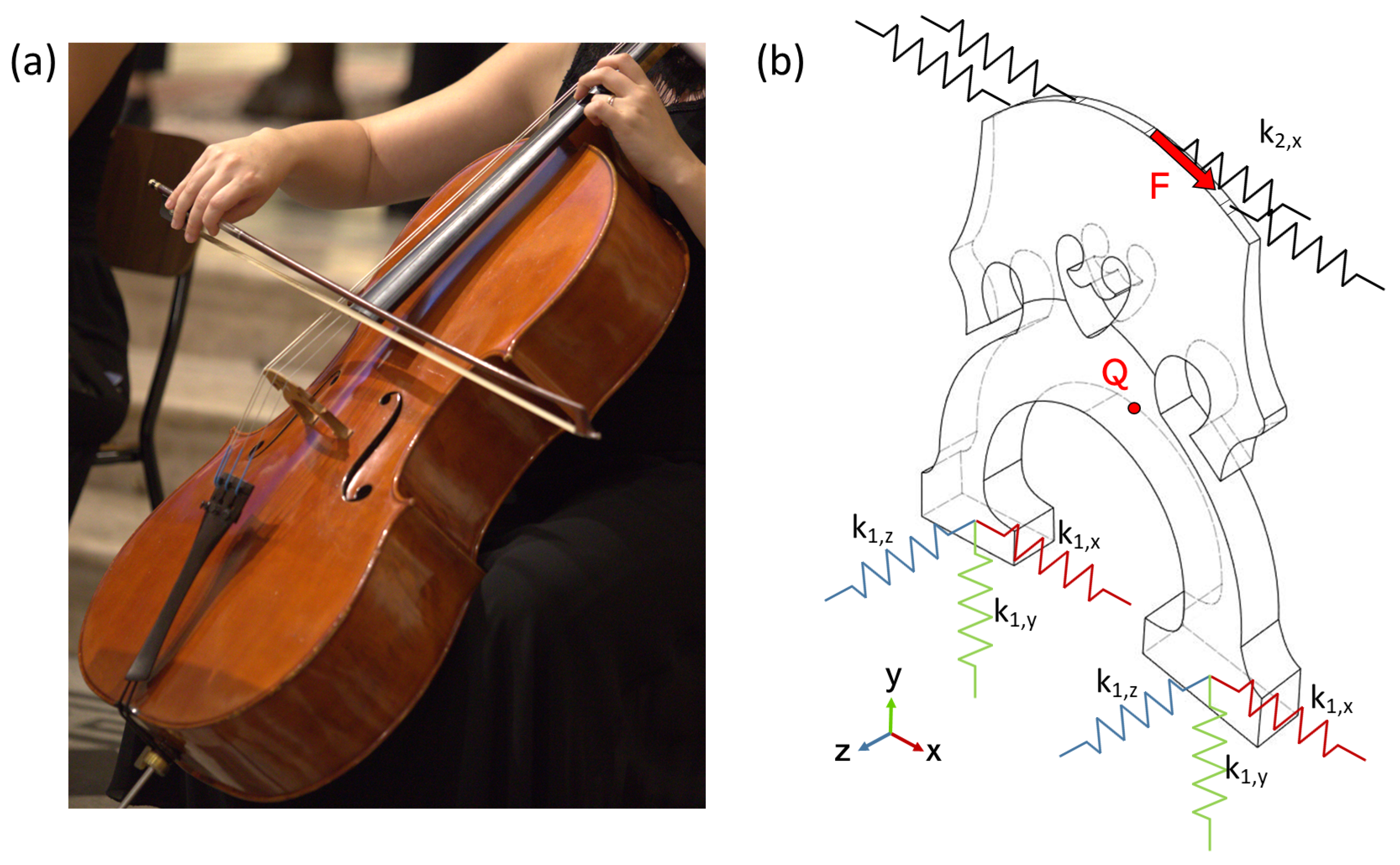
2.3. Boundary Conditions

We have studied four different boundary conditions to have an idea of the dynamic effect that the stiffening of the legs has on the vibrational response. The first case is the free boundary conditions, which correspond to the bridge blank not interacting with any other part of the cello. Then we modeled the interaction between the bridge, the body, and the strings in different ways, inspired by [14]. We defined u , v , w as the displacement in the directions of the x , y , z axes, respectively. First, we imposed a fixed boundary condition at the base of the feet ( u = v = w = 0 ), but we set no constraint on the point of contact with the strings. In a more realistic approach, instead of fixed boundary conditions, we implemented springs in three dimensions so as to represent the movement of the top plate, as depicted in Figure 2. Note that this is a coarse approximation, as we know that a cello has many more degrees of freedom. The spring constants in this case are k x 1 = 1.8 × 10 6 N/m, k y 1 = 0.1 × 10 6 N/m, and k z 1 = 7.7 × 10 6 N/m. We also set a scalar damping loss factor η s = 0.1 , such that the total force exerted by the springs with loss is f s l = ( 1 + i η ) f s , where f s is the elastic spring force. Finally, we implemented the boundary condition at the point of contact with the strings. Here, the bridge plate cannot move in the z direction, so we imposed w = 0 on the upper arch. Furthermore, a spring along the x direction was used to represent the force that the strings apply on the bridge. For the sake of simplicity, we modeled all the strings as exerting the same force, so that a single spring constant k x 2 = 0.1 × 10 6 N/m was needed. The values used have been taken from [14].

2.4. Forcing Term and Measure Point

To obtain the Frequency Response Function of the different models, and therefore a more complete picture of their behavior in frequency, we simulated a harmonic excitation force F of amplitude 1 N . F was applied to a small section of the upper arch of the bridge, modeling the notch that would accommodate the D string; it was tangential to the surface, with no component in the z direction (Figure 2). In this case, the feet were set as fixed. We also defined a point Q on the surface of the bridge and computed its displacement.

3. Results

We focused on the parametric dependence of the bridge response in two cases: the displacement under load and the vibrational response. Our idea was to understand how the modification of the legs curve affects the behavior of the bridge and if this change could help explain the subjective perception of the Amorim family, who observes that their model has a faster response.

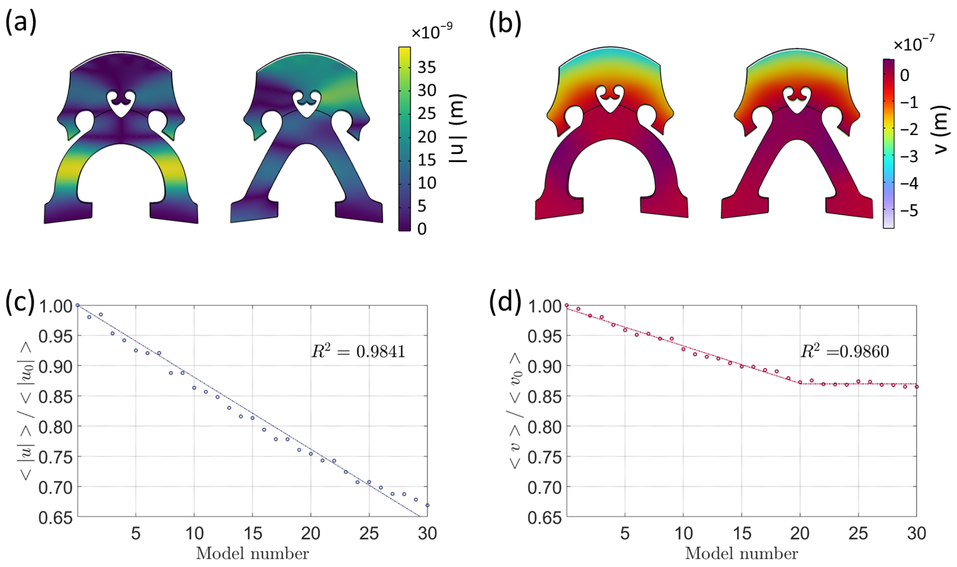
3.1. Static Behavior

Figure 3 shows the displacement of the bridge when the force of the strings is modeled through a nominal compression force, applied at the string notches in the y direction. The bridge displacement is a three-dimensional field, but most of it is observed on the x y plane. Figure 3a shows the displacement field | u | for the two extreme cases (Normal and Model 30) while Figure 3b shows the value of v in each point of the bridge. The two models present clear differences, especially in the distribution of | u | in the area of the legs.
In Figure 3c, the spatial average of | u | is plotted as a function of the model number. The displacement decays linearly with the model number. If we recall that in a spring the displacement is inversely proportional to the stiffness, we can conclude that the straightening of the legs corresponds to a stiffening of the bridge. In particular, the stiffness along the x direction increases by more than 50%. The v component shows a similar behavior but in a smaller range, as shown in Figure 3d. The displacement reaches a plateau around model 20, and the overall decrease is around 17% instead.

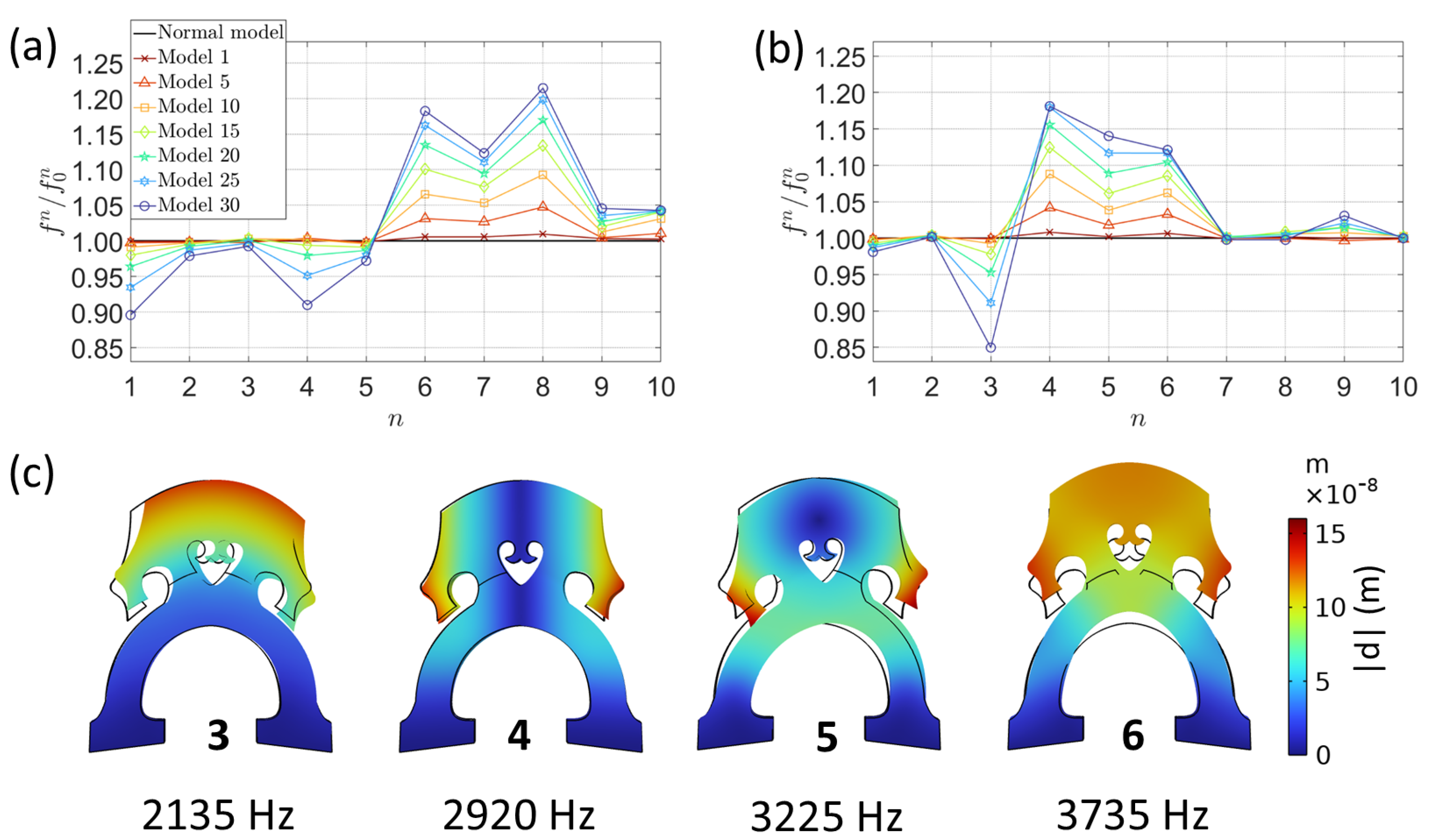
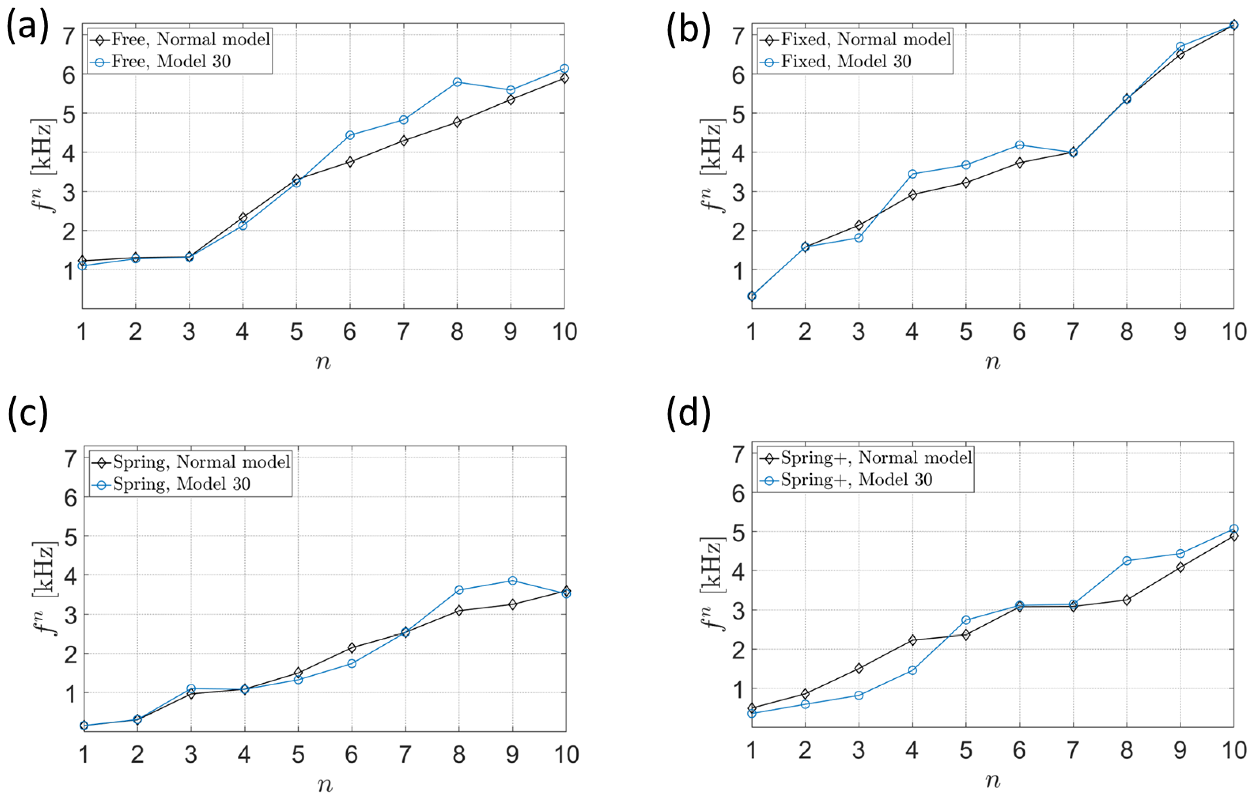
3.2. Eigenfrequency Study

Figure 4 shows the relative variation in the first ten eigenfrequencies for the (a) free and (b) fixed feet boundary conditions. In particular, the variation in the eigenfrequencies is normalized with respect to the Normal Model.
In free boundary conditions, the modal frequencies that change the most when varying the shape of the legs are associated with modes 1, 4, 6, 7, 8. The mode shapes associated with these modes present a displacement concentrated in the legs (Figure A2 and Figure A3). In particular, the mode shapes of modes 6 and 7 exhibit the most different mode shapes if we compare the Normal Model to Model 30.
In fixed boundary conditions, modes 3, 4, 5, and 6 are the most affected in terms of frequency by the change in the shape of the legs. The mode shapes associated with modes 3, 5, and 6 that occur in plane x y are also reported in other studies [9,15] as the most relevant.
A summary of the eigenfrequencies of the first 10 modes under different boundary conditions is given in Table 2 and Table 3. Figure 5 allows one to visualize the same eigenfrequencies and to compare them for each boundary condition. It is apparent that the boundary conditions have the largest impact on the natural frequencies. If the feet are fixed, the first frequency decreases by almost 1000 Hz with respect to the free boundary conditions. Something similar happens when using springs for the boundary conditions and there are many more modes in the mid-frequency range (1–4 kHz) than in the free boundary case. This dependence on the boundary conditions shows that it is not possible to directly obtain insights into how the bridge behaves in the cello from its free body behavior. Accurately describing the boundary conditions of a real instrument goes far beyond the scope of this article and should be tackled in future research.

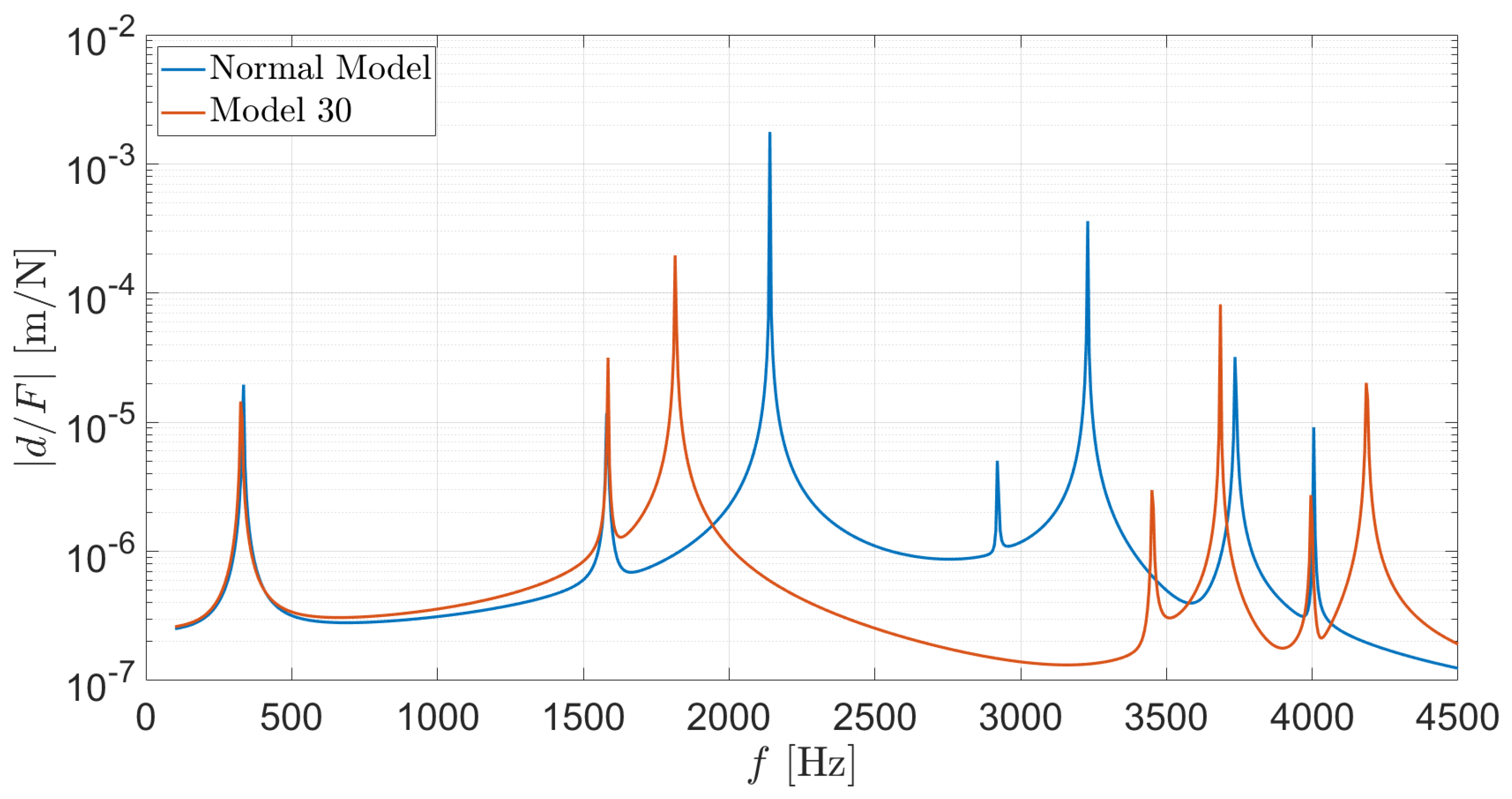
3.3. Frequency Response Function

Figure 6 shows the amplitude of the FRF of the bridge, obtained from the displacement d of the point Q when the force F is applied. Consistently with the previous results, the FRF peaks correspond to the values of eigenfrequencies of Table 2 and Table 3. The first two modes are not particularly affected by the leg modification, while in the frequency range 1500–3500 Hz, aside from the differences in the locations of the peaks, a decrease in magnitude is clearly noticeable from the Normal Model to Model 30. From the eigenfrequency analysis, we know there is a continuous (albeit non-linear) shifting of the third mode as the parametric model changes. The eigenfrequency does not practically change for the first 10 models and has a rapid variation in the last five. The vibrational response for the intermediate models is consistent with this change in eigenfrequency, and the amplitude follows suit. This particular variation in a single mode is quite relevant as it would allow the instrument maker to tune the response of the instrument in the middle range without having to modify the structure of the instrument, only the set-up.

4. Conclusions

In this article, we have shown by means of finite element modeling that changing the design of the cello bridge is akin to stiffening its material. The variation in apparent stiffness has a linear dependence with the parameter controlling the shape variation of the legs. The range of values of the stiffness reachable with this varying geometry corresponds to a 50% increase in the longitudinal stiffness and a 17% increase in the radial stiffness. Furthermore, when looking at the admittance of the bridge, we have found that the response in the mid-range can be continuously controlled by changing the geometric parameter. This would allow the instrument maker to fine tune the response of an instrument in a particular frequency range without having to make structural changes to the instrument, only to the setup.
An aspect that we have not studied in this article is the influence on the sound and playability due to design variations. We know that changing the shape of the bridge will shift the position of the modes in the so-called “bridge hill” region [16], so we expect a change in the mid-range components of the sound. According to the musicians who have tried this model, the cello has a faster response and it is “easier” to play. This points towards a change in the minimum bow force due to the change in bridge resonances [17]. These are exciting subjects of research we are currently pursuing experimentally. To facilitate studies like this by other groups, our code and models are freely available online (See Data Availability Statement).
The implications of this research in instrument-making could be far reaching: we have found a simple way to compensate for variations in the material by a continuous geometrical parameter. The material parameters of a given blank can be easily estimated by tapping experiments, and thanks to the results presented here, the shape required for the desired stiffness can be easily computed. This is another step in our efforts of bringing cutting edge technology to a 300-year-old craft.
This paper has shown how the intuition and embodied knowledge of luthiers can help guide scientific research and how science can give an objective correlate to the subjective intuitions of the experts in the field. Rather than disregarding the know-how of instrument makers, this article aims to show that both kinds of knowledge can work together and complement each other to achieve new insights.

Author Contributions

Conceptualization, project administration, and supervision, S.G.; investigation, software, data curation, and visualization, L.L.; methodology and formal analysis, S.G. and L.L.; writing—original draft, S.G and L.L.; writing—review and editing, L.L and S.G.; funding acquisition, F.A. and A.S. All authors have read and agreed to the published version of the manuscript.

Funding

This research was funded by the MSCA EF 2020 grant of Politecnico di Milano.

Institutional Review Board Statement

Not applicable.

Informed Consent Statement

Not applicable.

Data Availability Statement

Data relevant to the study (for example, CAD and COMSOL Multiphysics files) are available at https://github.com/LauraLodetti/Cello_bridges (Accessed: 4 January 2023). Moreover, a short video containing animations can be viewed on YouTube https://youtu.be/JTxqf4hO2vA (Accessed: 4 January 2023).

Acknowledgments

We thank the Amorim family for their openness and willingness to engage in this research and C. Espinoza for the critical reading of the manuscript.

Conflicts of Interest

The authors declare no conflict of interest.

Appendix A

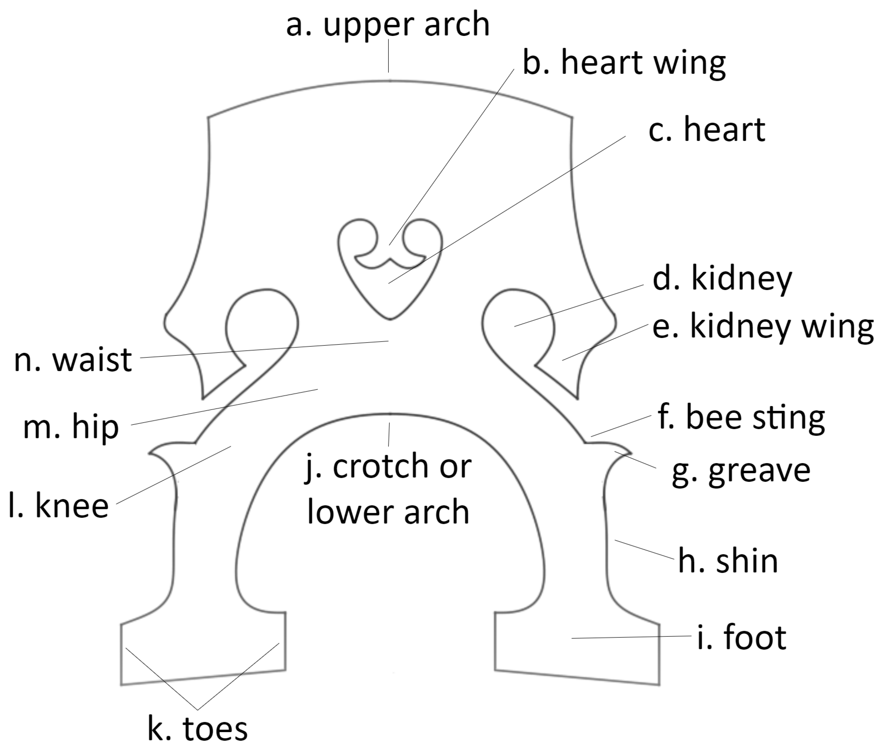
Appendix A.1. Terminology

Figure A1. Outline of a French cello bridge and the names of the different parts.
Applsci 13 00928 g0a1

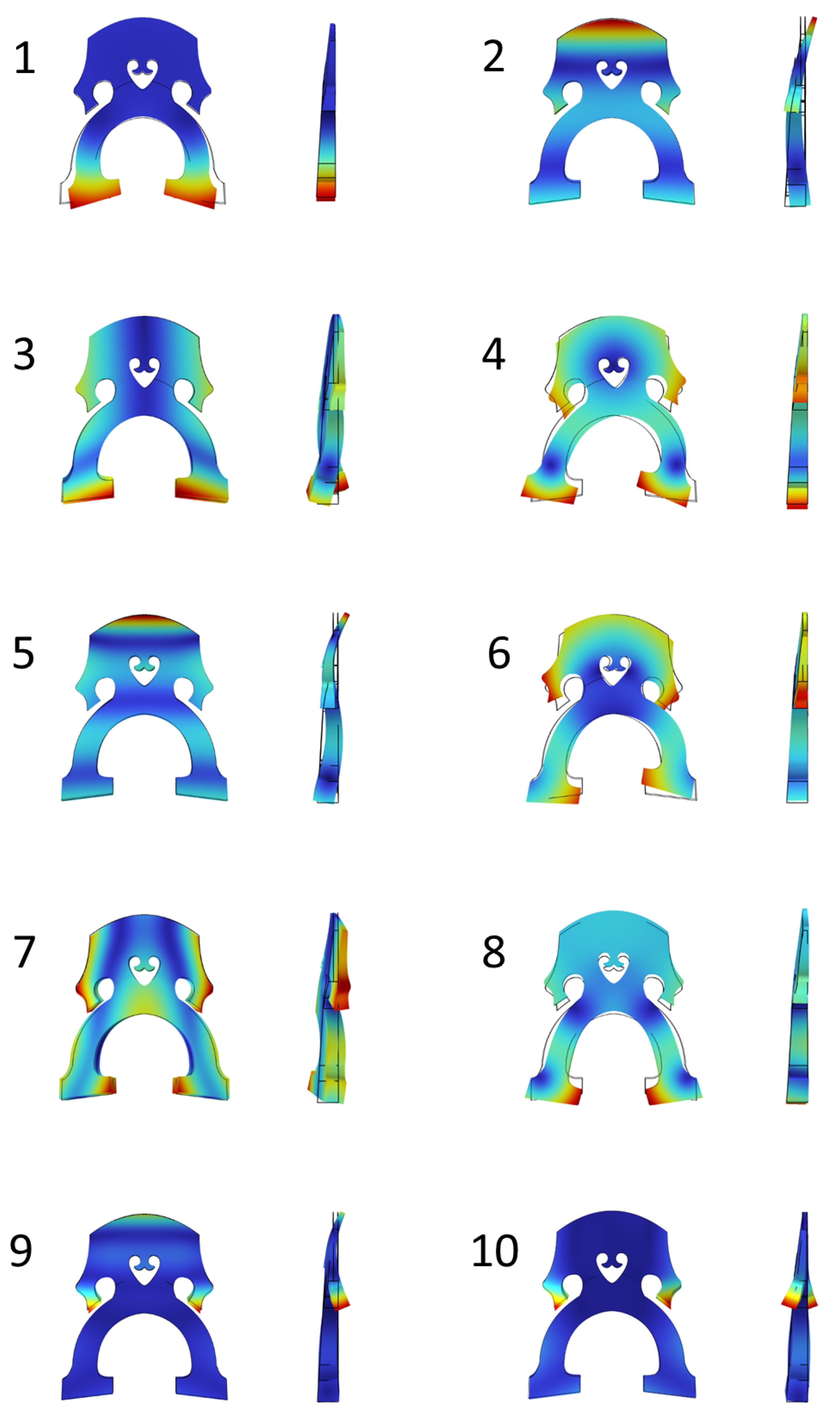
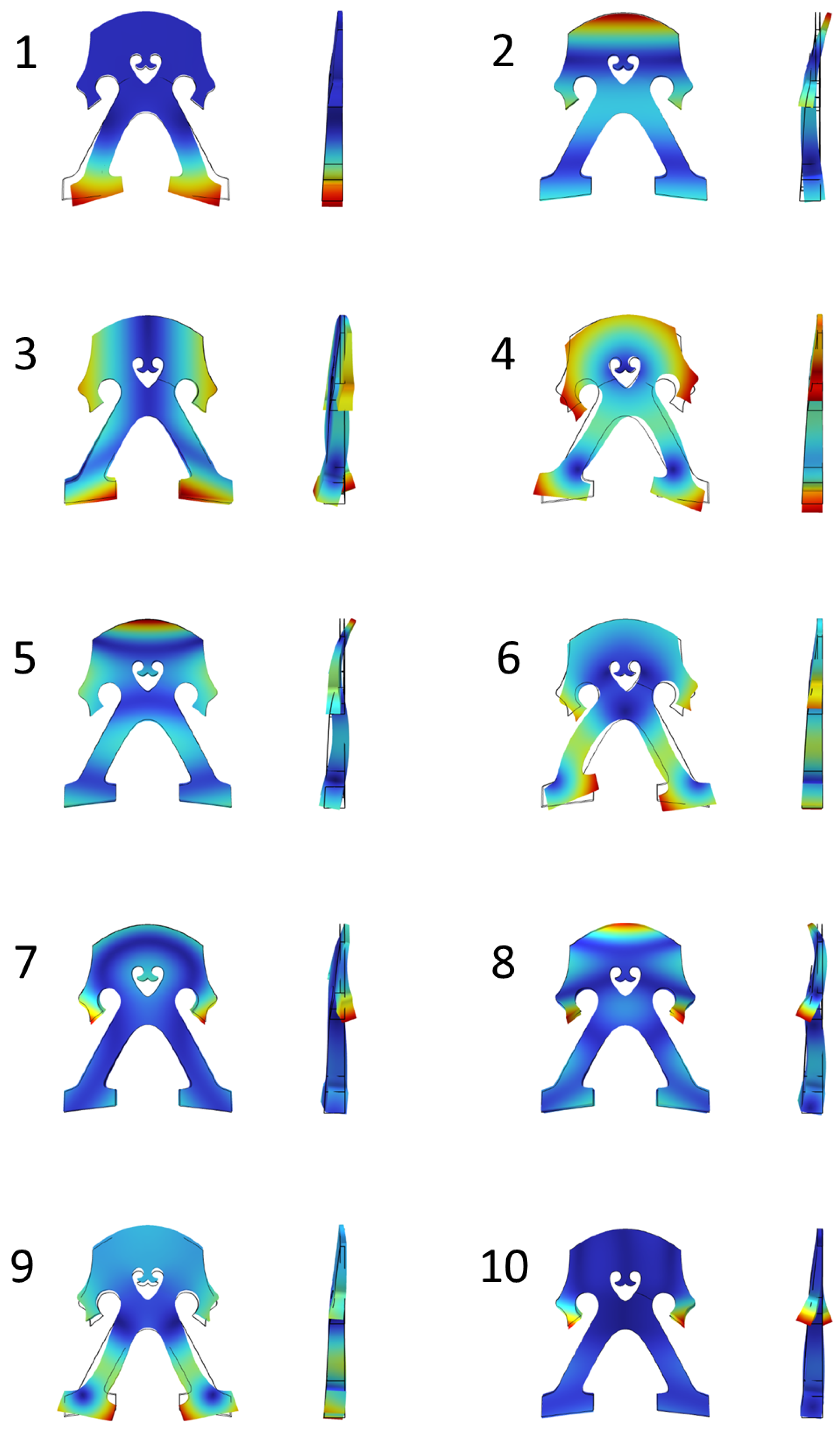
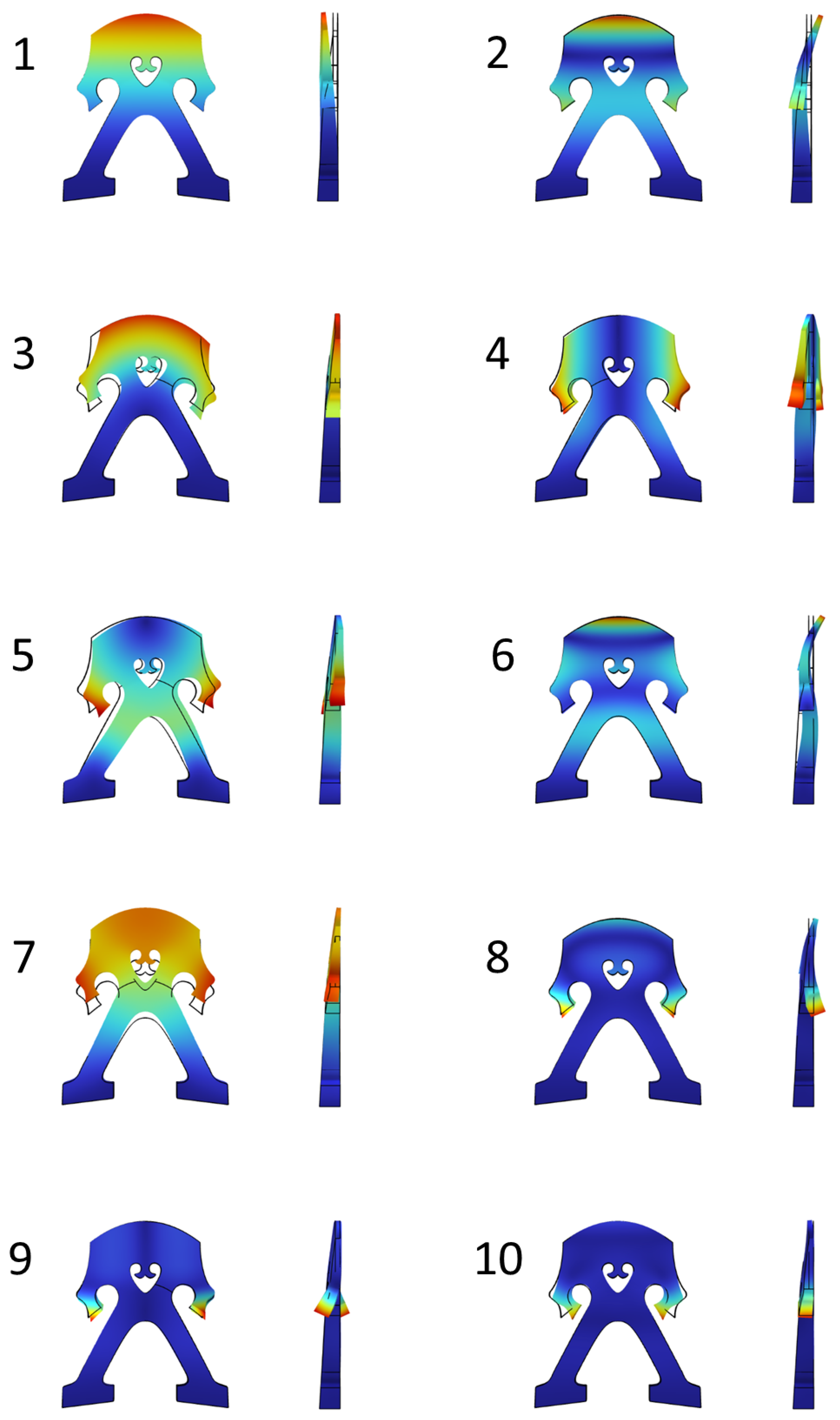
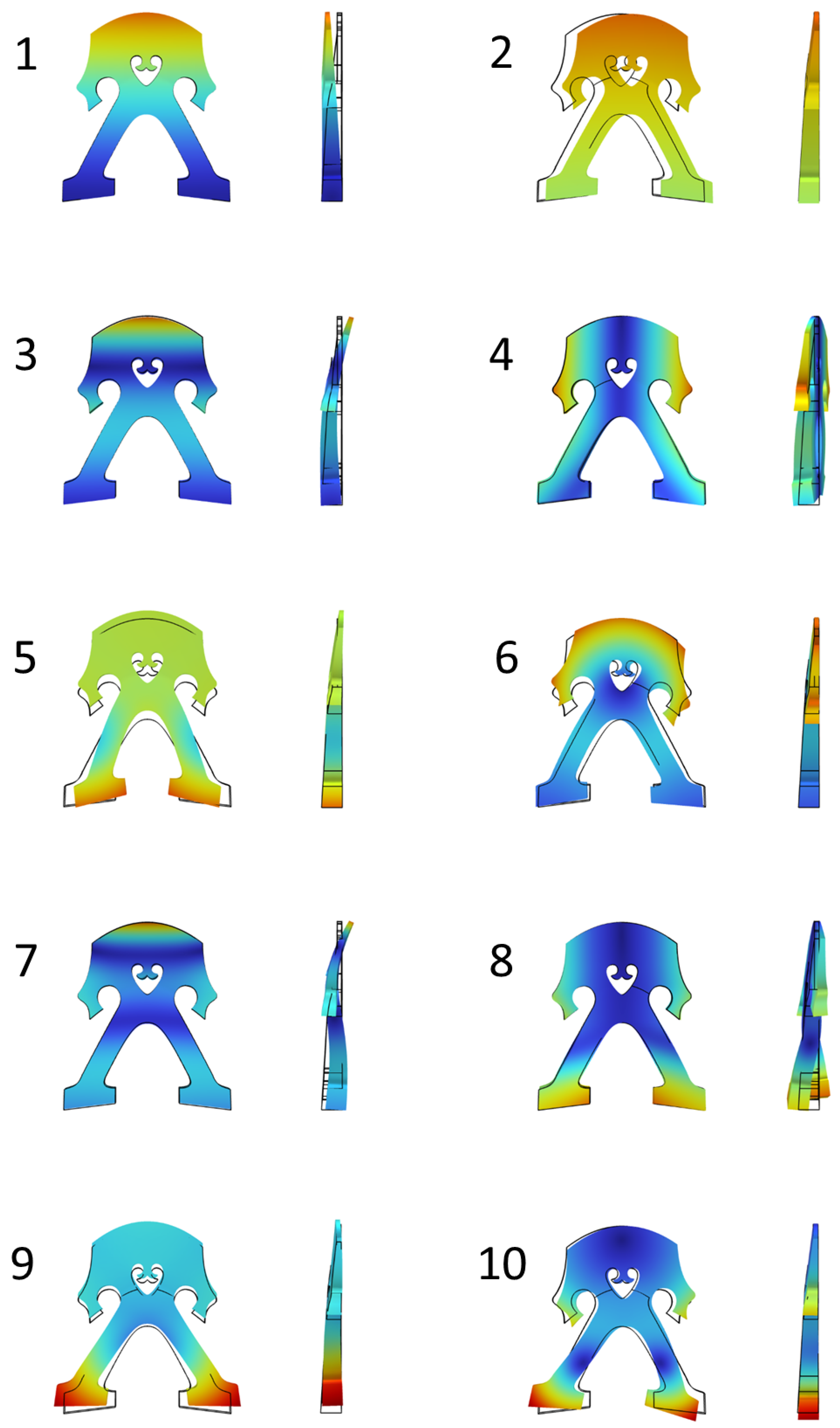
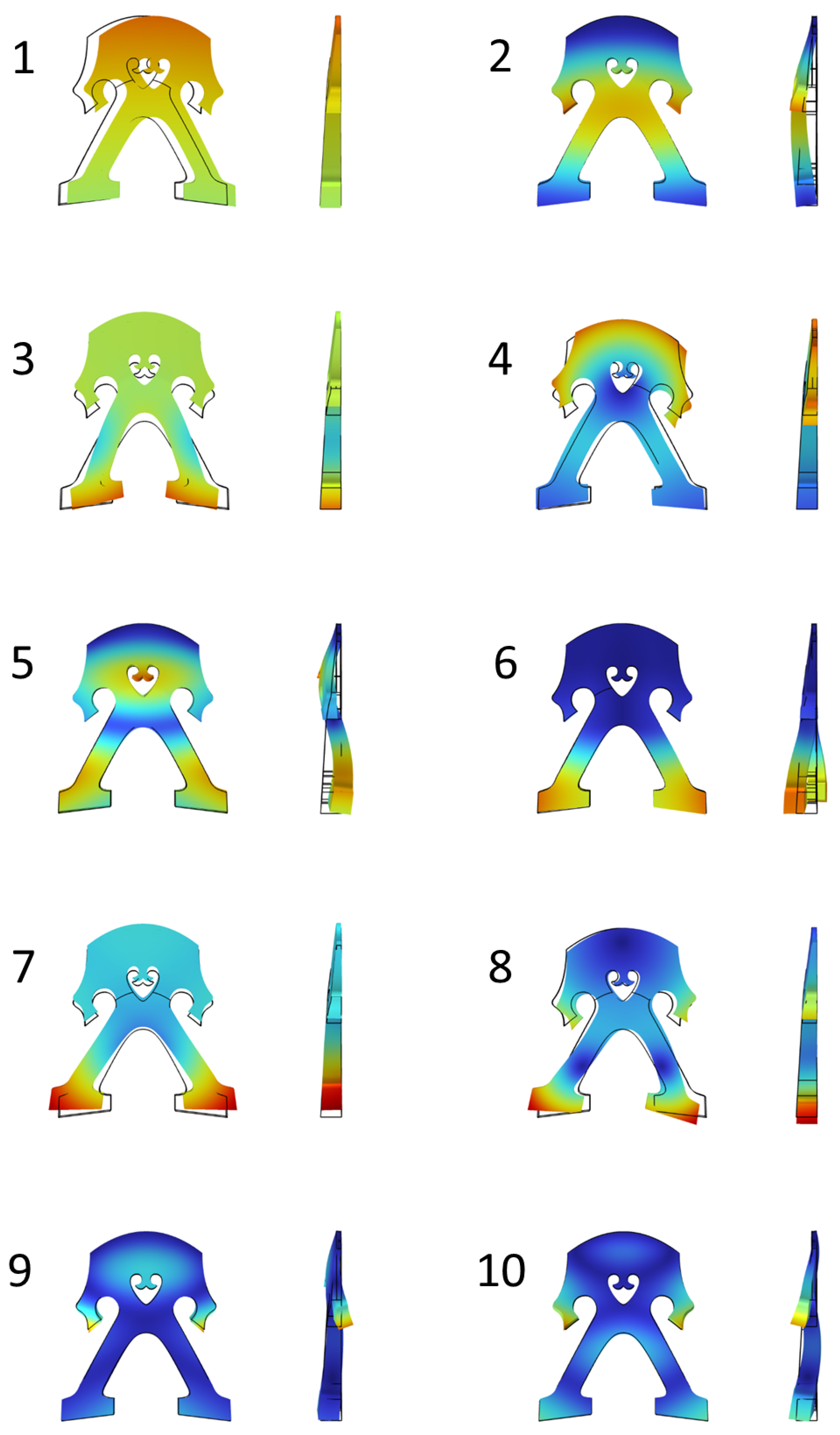
Appendix A.2. Mode Shapes

The figures in this section contain all the mode shapes for the Normal Model and Model 30 in all the different boundary conditions considered. We also describe the modes in the case of free boundary conditions and point out mode switches and/or relevant observations.
The images are meant to be used as a reminder of what the mode shape looks like and to help the comparison between different models and boundary conditions in a quick way; however, they might prove hard to follow. A video that shows animations for all of them is available online on https://youtu.be/JTxqf4hO2vA (Accessed: 4 January 2023) or at https://github.com/LauraLodetti/Cello_bridges (Accessed: 4 January 2023).
Figure A2 shows mode shapes in free boundary conditions, for the Normal model. Mode 1: The feet move inward and outward in the xy-plane, symmetrically with respect to the y-axis.
Mode 2: Two horizontal nodal lines are noticeable at the shins and at the heart of the bridge, respectively. The upper arch of the bridge has greater displacement with respect to the waist and the feet.
Mode 3: A central vertical nodal line is combined with two nodal lines at the shins. A sort of “walking” mode, where the left side (mostly the kidney wing, the knee, the foot) and the right side move in opposite phase in the z direction.
Mode 4: Three nodal points are present (one over the heart, two on the shins). The feet oscillate around the nodal points on the xy-plane, in phase with each other. The portion of the bridge around the waist rotates in counter phase around the nodal point over the heart.
Mode 5: Similar to Mode 2, but with three horizontal nodal lines (above the heart, at the waist, at the shins).
Mode 6: One nodal point at the waist and two nodal points at the outer conjunction between the shins and the feet. The inner toes move up and down, with opposite phase. The upper arch rotates around the nodal point.
Mode 7: Two symmetrical nodal lines start from the upper arch, pass beside the heart and the hip, and continue down the legs. The motion is out of the xy-plane, with kidney wings in phase with each other and in opposite phase with the crotch and the inner toes.
Mode 8: Internal toes displace symmetrically around a nodal point on the outer shin and are accompanied by an up-and-down motion (with opposite phase) of the whole region above the waist.
Mode 9: Four horizontal node lines (one above the heart, one just below the heart and above the kidney wings, one just below the waist and one at the connection of shins and feet). The displacement of the kidney wing is noticeably greater than the one of the legs.
Mode 10: Movement in the z direction of the kidney wings, accompanied by smaller z movement of the legs. Opposite leg and kidney wing are in phase, in a sort of “walking in place” mode.
Figure A3 shows the mode shapes for Model 30, again in free boundary conditions. Mode shapes for modes 1, 2, 3, and 10 are very similar to the Normal Model. Modes 4, 5 and 6 present small differences: in mode 4, the nodal points move slightly upwards in y direction; in mode 5, the nodal lines appear more curved, as if going towards an x shape; and in mode 6, the movement of the legs and of the feet is more enhanced. There is a mode switch between mode 8 and 9, where in mode 8, the nodal lines go towards an x shape, and in mode 9, the nodal points in the feet move towards the center.
Figure A4 shows the mode shapes of the Normal Model, in case of fixed boundary conditions. As expected, mode shapes differ from the ones in free boundary conditions. Mode 1: Back-and-forth, out-of-plane motion of the upper portion of the bridge.
Mode 2: One horizontal nodal line.
Mode 3: Sideways rotation of the portion above the heart.
Mode 4: Motion similar to mode 3 in free boundary conditions, with a vertical nodal line at the center and alternated back-and-forth motion of the kidney wings.
Mode 5: Rocking motion of the waist of the bridge, with a nodal point slightly above the heart.
Mode 6: Up and down motion of the upper portion of the bridge.
Mode 7: Out-of-plane mode shape with two horizontal nodal lines.
Mode 8: Ring mode, with kidney wings and upper arch moving out of phase with respect to the heart.
Mode 9: Back-and-forth alternate motion of the kidney wings, with a vertical nodal line.
Mode 10: In-plane inwards and outwards motion of the kidney wings, symmetrical with respect to the y-axis.
Figure A5 shows the mode shapes of Model 30, in case of fixed boundary conditions. Mode shapes remain very similar to the Normal Model, except for a mode switch between mode 6 and mode 7.
Figure A6 and Figure A7 show the mode shapes of the Normal Model and Model 30 respectively, in case of Spring feet boundary conditions (defined as case (c)). Mode shapes in this case present similarities to the previous ones, but interestingly, a rigid motion (translation in x direction) appears in mode 2.
Figure A8 and Figure A9 show the mode shapes of the Normal Model and Model 30 respectively, in case of Spring boundary conditions both on the feet and the upper arch of the bridge (defined as case (d)). A rigid motion, similar to the one of the second mode of the previous case, appears here on the first mode.
Figure A2. Mode shapes in free boundary conditions (case (a)) for the Normal Model.
Applsci 13 00928 g0a2
Figure A3. Mode shapes in free boundary conditions (case (a)) for Model 30.
Applsci 13 00928 g0a3
Figure A4. Mode shapes in fixed boundary conditions (case (b)) for the Normal Model.
Applsci 13 00928 g0a4
Figure A5. Mode shapes in fixed boundary conditions (case (b)) for Model 30.
Applsci 13 00928 g0a5
Figure A6. Mode shapes in spring boundary conditions (case (c)) for the Normal Model.
Applsci 13 00928 g0a6
Figure A7. Mode shapes in spring boundary conditions (case (c)) for Model 30.
Applsci 13 00928 g0a7
Figure A8. Mode shapes in spring boundary conditions (case (d)) for the Normal Model.
Applsci 13 00928 g0a8
Figure A9. Mode shapes in spring boundary conditions (case (d)) for Model 30.
Applsci 13 00928 g0a9

References

  1. Raymaekers, W. Bridge shapes of the violin and other bowed instruments, 1400–1900: The origin and evolution of their design. Early Music 2020, 48, 225–250. [Google Scholar] [CrossRef]
  2. Fletcher, N.H.; Rossing, T.D. The Physics of Musical Instruments; Springer Science & Business Media: New York, NY, USA, 2012. [Google Scholar]
  3. Rossing, T.D. (Ed.) The Science of String Instruments; Springer: New York, NY, USA, 2010. [Google Scholar]
  4. Müller, H. The function of the violin bridge. Catgut Acoust. Soc. Newsl. 1979, 31, 19–22. [Google Scholar]
  5. Gough, C. Violin plate modes. J. Acoust. Soc. Am. 2015, 137, 139–153. [Google Scholar] [CrossRef] [PubMed] [Green Version]
  6. Gonzalez, S.; Salvi, D.; Baeza, D.; Antonacci, F.; Sarti, A. A Data-driven Approach to Violin Making. Sci. Rep. 2021, 11, 9455. [Google Scholar] [CrossRef] [PubMed]
  7. Salvi, D.; Gonzalez, S.; Antonacci, F.; Sarti, A. Parametric optimization of violin top plates using machine learning. In Proceedings of the 27th International Congress on Sound and Vibration, ICSV 2021, Virtual, 11–16 July 2021. [Google Scholar]
  8. Marschke, S.; Wunderlich, L.; Ring, W.; Achterhold, K. An approach to construct a three-dimensional isogeometric model from µ-CT scan data with an application to the bridge of a violin. Comput. Aided Geom. Des. 2020, 78, 1–19. [Google Scholar] [CrossRef]
  9. Rodgers, O.; Masino, T. The effect of wood removal on bridge frequencies. Catgut Acoust Soc. J. 1990, 1, 6–10. [Google Scholar]
  10. Gonzalez, S.; Salvi, D.; Antonacci, F.; Sarti, A. Eigenfrequency Optimisation of Free Violin Plates. J. Acoust. Soc. Am. 2021, 149, 1400–1410. [Google Scholar] [CrossRef] [PubMed]
  11. Lercari, M.; Gonzalez, S.; Espinoza, C.; Longo, G.; Antonacci, F.; Sarti, A. Using Metamaterials in Guitar Top Plates: A Numerical Study. Appl. Sci. 2022, 12, 8619. [Google Scholar] [CrossRef]
  12. Gonzalez, S.; Chacra, E.; Carreño, C.; Espinoza, C. Wooden Mechanical Metamaterials: Towards tunable wood plates. Mater. Des. 2022, 221, 110952. [Google Scholar] [CrossRef]
  13. Kaselouris, E.; Bakarezos, M.; Tatarakis, M.; Papadogiannis, N.A.; Dimitriou, V. A Review of Finite Element Studies in String Musical Instruments. Acoustics 2022, 4, 183–202. [Google Scholar] [CrossRef]
  14. Kabała, A.; Niewczyk, B.K.; Gapiński, B. Violin bridge vibrations—FEM. Vib. Phys. Syst. 2018, 29, 1–7. [Google Scholar]
  15. Gi-Sang, C. Analysis of Vibration in Cello Bridge. J. Acoust. Soc. Korea 2006, 25, 197–206. [Google Scholar]
  16. Woodhouse, J. On the “bridge hill” of the violin. Acta Acust. United Acust. 2005, 91, 155–165. [Google Scholar]
  17. Mansour, H.; Woodhouse, J.; Scavone, G.P. On minimum bow force for bowed strings. Acta Acust. United Acust. 2017, 103, 317–330. [Google Scholar] [CrossRef]
Figure 1. (a) Picture of a French model cello bridge blank (courtesy of luthier Matteo Pontiggia). (b) Picture of Amorim’s Model X blank during the final construction stages (courtesy of luthier Luiz Amorim). (c) Three examples of our 3D model and its evolution as we vary the control parameter of the legs.
Applsci 13 00928 g001
Figure 2. (a) Picture of a cellist playing the D string sul tasto, meaning that the bow is near the fingerboard. Ideally, when bowing the instrument, the player applies a force F perpendicular to the string. (b) Schematic representation of spring locations used as boundary conditions. In addition, the figure shows the location of point Q and the force vector F, used for the FRF. The figure shows the Normal Model but is valid for all models.
Applsci 13 00928 g002
Figure 3. Displacement fields on the bridge under load. (a) Magnitude of the displacement along the x direction. (b) Displacement along the y direction. (c) Spatial average of the displacement along the x direction normalized for the Normal Model, as a function of the model number. The equation of the linear fitting curve is f ( m ) = 0.0119 m + 1 . (d) Spatial average of the displacement along the y direction normalized for the Normal Model, as a function of the model number. The equation of the piecewise linear fitting curve is f ( m ) = 0.0062 m + 0.9946 for m 20 , f ( m ) = 0.8699 for m > 20 . The R-squared refers to the first portion of the fit, as the constant value in the second portion is the mean.
Applsci 13 00928 g003
Figure 4. (a) Changes in natural frequencies f n in free boundary conditions. (b) Variation in natural frequencies f n in fixed boundary condition. Frequencies from different models are shown as a function of the mode number n; f 0 n is the frequency of the nth mode for the Normal Model. (c) Mode shapes and corresponding natural frequencies for n = 3 , , 6 in constrained boundary conditions, | d | being the norm of displacement, shown on the Normal Model.
Applsci 13 00928 g004
Figure 5. Modal frequencies as a function of the mode number, from Table 2 and Table 3. Note that in this case, eigenfrequencies are rearranged in order to take care of mode switches. Each plot compares the values obtained for the Normal model and Model 30 in a specific boundary condition. (a) Free boundary conditions. (b) Fixed boundary conditions. (c) Boundary condition with springs at the feet only. (d) Boundary condition with both springs at the feet and at the upper arch.
Applsci 13 00928 g005
Figure 6. Frequency Response Function of the Normal Model and of Model 30. The FRF is computed between the nominal excitation force F and the displacement d of point Q, located at the hip of the bridge. The frequency resolution is 5 Hz.
Applsci 13 00928 g006
Table 1. Mechanical parameter values of the simulated material, taken from [9]. Density ρ is assumed to be equal to 700 kg/m 3 .
Young’s ModulusRigidity ModulusPoisson’s Ratio
E x = 10.00 GPa G x y = 1.60 GPa ν x y = 0.38
E y = 2.00 GPa G y z = 0.72 GPa ν y z = 0.47
E z = 1.20 GPa G z x = 1.60 GPa ν z x = 0.48
Table 2. Values of the first 10 natural frequencies (in H z ) of the Normal Model in different boundary conditions. Case (c) only includes springs at the feet, while case (d) both springs at the feet and at the upper arch. Modes where the bridge moves rigidly are denoted with r m . All mode shapes are available in Figure A2, Figure A4, Figure A6, and Figure A8.
Mode Number(a) Free(b) Fixed(c) Spring(d) Spring+
11227333160498 r m
213111580309 r m 861
3133123169681597
42337291810902231
53306322415072364
63753373421493076
74298400325353083
84768536930873250
95347650432464082
105889725235924887
Table 3. Values of the first 10 natural frequencies (in H z ) of Model 30 in different boundary conditions. Modes where the bridge moves rigidly are denoted with r m . Mode switches with respect to the Normal Model in the same boundary conditions are in bold. All mode shapes are available in Figure A3, Figure A5, Figure A7, and Figure A9.
Mode Number(a) Free(b) Fixed(c) Spring(d) Spring+
11099327162317 r m
212831583317 r m 870
31320181511061331
42126344710851747
53212367713302459
64437418617443145
74827399425363617
85590535638563859
95791670435164127
106140725136144643
Disclaimer/Publisher’s Note: The statements, opinions and data contained in all publications are solely those of the individual author(s) and contributor(s) and not of MDPI and/or the editor(s). MDPI and/or the editor(s) disclaim responsibility for any injury to people or property resulting from any ideas, methods, instructions or products referred to in the content.

