Abstract
The reptile search algorithm is a newly developed optimization technique that can efficiently solve various optimization problems. However, while solving high-dimensional nonconvex optimization problems, the reptile search algorithm retains some drawbacks, such as slow convergence speed, high computational complexity, and local minima trapping. Therefore, an improved reptile search algorithm (IRSA) based on a sine cosine algorithm and Levy flight is proposed in this work. The modified sine cosine algorithm with enhanced global search capabilities avoids local minima trapping by conducting a full-scale search of the solution space, and the Levy flight operator with a jump size control factor increases the exploitation capabilities of the search agents. The enhanced algorithm was applied to a set of 23 well-known test functions. Additionally, statistical analysis was performed by considering 30 runs for various performance measures like best, worse, average values, and standard deviation. The statistical results showed that the improved reptile search algorithm gives a fast convergence speed, low time complexity, and efficient global search. For further verification, improved reptile search algorithm results were compared with the RSA and various state-of-the-art metaheuristic techniques. In the second phase of the paper, we used the IRSA to train hyperparameters such as weight and biases for a multi-layer perceptron neural network and a smoothing parameter (σ) for a radial basis function neural network. To validate the effectiveness of training, the improved reptile search algorithm trained multi-layer perceptron neural network classifier was tested on various challenging, real-world classification problems. Furthermore, as a second application, the IRSA-trained RBFNN regression model was used for day-ahead wind and solar power forecasting. Experimental results clearly demonstrated the superior classification and prediction capabilities of the proposed hybrid model. Qualitative, quantitative, comparative, statistical, and complexity analysis revealed improved global exploration, high efficiency, high convergence speed, high prediction accuracy, and low time complexity in the proposed technique.
1. Introduction
Metaheuristics are stochastic search algorithms inspired by the natural phenomenon of biological evolution and human behaviors. Metaheuristics (MH) are simple, flexible, and derivative-free techniques that can efficiently solve various challenging, non-convex optimization problems. The meta-heuristic algorithm solves the optimization problem by considering only the input and output of the base system defined as an optimization problem and does not require a strict mathematical model. Therefore, metaheuristic algorithms are very successful in solving real-world optimization problems with complex information [1,2,3].
The meta-heuristic techniques can be divided into two main classes: evolutionary algorithms (EA) and swarm intelligence (SI) algorithms. EAs are based on the theory of evolution and natural selection, which is a way of explaining how species change over time. Examples of classical evolutionary computing techniques are genetic algorithm (GA), evolution strategy (ES), simulated annealing (SA), differential evolution (DE), and genetic programming (GP) [4,5]. SI algorithms mimic social interactions in nature (such as animals, birds, and insects) [6]. Some of the well-known SI methods include particle swarm optimization (PSO), salp swarm optimization (SSA) [7], ant colony optimization (ACO) [8], firefly algorithm (FA), and whale optimization algorithm (WOA) [9].
There has been a sudden rise in the popularity of machine learning-based techniques within the past few decades. The performance of many areas, such as self-driving vehicles, medical, industrial manufacturing, image recognition, etc., has been greatly improved because of machine learning [10]. Machine learning is a computational process, and its main objective is to recognize different patterns in a relatively random set of data. Several machine learning methods like logical regression, naïve Bayes (NB), k-nearest neighbors (k-NN), decision trees, artificial neural network (ANN), and support vector machines (SVM) [11,12,13] are available in the literature for solving various classification and regression problems.
ANNs are one of the most famous and practical machine learning methods developed to solve complex classification and regression problems. An ANN is a computational model which is biologically inspired. It consists of neurons, which are the processing elements, and the connections between them, which have some values known as weights [14]. Neurons are usually connected by these weighted links over which information can be processed. The main characteristics of a neural network are learning and adaptation, robustness, storage of information, and information processing [15]. ANNs are widely used in areas where traditional analytical models fail because either the data is not precise or the relationship between different elements is very complex. ANNs are used in pattern recognition [16,17,18], signal processing [19], intelligent control [20], and fault detection in electrical power systems [21,22,23]. Therefore, by applying ANNs to different fields, we can optimize the performance, and this has been a major research focus for the last few years.
The performance of a neural network depends upon the construction of the network, the algorithms used for training, and the choice of the parameters involved. Usually, gradient-based methods like backpropagation, gradient descent, Levenberg Marquardt back propagation (LM), and scaled conjugate gradient (SCG) are used to train neural networks. However, these classical methods are highly dependent on initial solutions and may trap in the local minima resulting in performance degradation [24]. Therefore, to enhance performance, evolutionary computing techniques can be applied to train neural networks. These networks are known as Evolutionary Neural Networks.
With the rapid development in computing techniques, a variety of metaheuristic search methods have been used for the optimal training of neural networks [24,25,26]. The basic inspiration for these metaheuristic search methods is the natural phenomenon of biological evolution and human behaviors. Metaheuristic algorithms consider different parameters of ANN as an optimization model and then make an effort to find a near-optimal solution [27]. Due to the added benefit of the powerful global and local searching capabilities of metaheuristic algorithms, the hybrid ANN is becoming a great tool for solving different classification and regression problems.
1.1. Contributions and Organization
According to the no free lunch theorem (NFL) [28], no metaheuristic algorithm can efficiently solve all optimization problems. An algorithm that gives excellent results for one optimization problem may perform poorly when applied to another optimization problem. This inequality was the motivation for this research. The main work of this paper was based on the refinement of the biologically inspired reptile search algorithm (RSA) [29]. In an extensive application, we applied this algorithm to solving various regression and classification problems.
RSA is a newly developed optimization technique that can efficiently solve various optimization problems. However, when applied to highly multidimensional nonconvex optimization problems like neural network training, the algorithm shows prominent shortcomings, such as stagnation at local minima, slow convergence speed, and high computational complexity. Therefore, in this paper, some improvements are proposed to make up for the above-mentioned drawbacks.
The reason for local minima stagnation is the lack of exploration in the high-walking stage of the RSA algorithm. Local minima trapping can be avoided if the solution candidates explore the search space as widely as possible. Therefore, to enhance exploration, a sine operator was included in the high walking stage of the RSA algorithm. The modified sine operator with enhanced global search capabilities avoids local minima trapping by conducting a full-scale search of the solution space.
The second innovation was designed to enhance the convergence capabilities in the hunting phase of the RSA algorithm. The Levy flight operator with jump size control factor was used to increase the exploitation capabilities of the search agents. The lower value of results in small random steps in the hunting phase of IRSA. This enables the solution candidates to search the area nearest to the obtained solution, which greatly improves the convergence capabilities of the algorithm.
As compared to the other state-of-the-art optimization algorithms, the computational complexity of RSA is very high. This time complexity limits the application of the algorithm in solving high-dimensional complex optimization algorithms. In the original RSA, the major causes of the complexity are the hunting operator and the reduce function . Especially while computing , division by a small value, , greatly increases the computational time of the algorithm. However, in the proposed algorithm with the above-mentioned improvisation, there was no need to calculate these complex operators, and they were excluded from the algorithm. This results in an almost 3-to-4-fold reduction in time complexity.
Thus, the proposed novel IRSA algorithm gives two benefits. First, there was a 10 to 15% improved performance as compared to the original RSA (experimentally verified in Section 3.2). Second, there was a 3-to-4-fold reduction in time complexity as compared to the original RSA (experimentally verified in Section 3.3). The major contributions of the research are:
- An improved reptile search algorithm (IRSA) based on a sine operator and Levy flight was proposed to enhance the performance of the original RSA.
- The proposed IRSA was evaluated using 23 benchmark test functions. Various qualitative, quantitative, comparative, statistical, and complexity analyses were performed to validate the positive effects of the improvisations.
- This research also proposed a hybrid methodology that integrates Multi-Layer Perceptron Neural Network with the improvised RSA for solving various classification problems.
- Finally, the IRSA was applied to train a radial basis function neural network (RBFNN) for short-term wind and solar power predictions.
The remaining article is assembled into seven sections. The proposed methodology is explained in Section 3. Section 4 delineates the effectiveness of the proposed IRSA through the performance of various experimental and statistical studies, along with comparisons. Section 4 also gives a brief rundown on the theoretical basis of the multi-layer perceptron neural network (MLPNN), radial basis function neural network (RBFNN), and proposed improved reptile search algorithm based neural network (IRSANN). Section 5 and Section 6 describe applications of the proposed technique in solving real-world classification and regression problems. Finally, Section 7 concludes the research.
1.2. Literature Survey
In the literature, various metaheuristic optimization techniques have been proposed and investigated for the training of the artificial neural network. The research in [30] used a hybrid AI model to predict the speed of wind at different coastal locations where PSO was applied to train an ANN. A comparison was made between the support vector machine, ANN, and hybrid ANN based wind speed prediction models, and it was observed that the root mean square error (RMSE) was the minimum for the hybrid PSOANN model. In [31], a hybrid ANN-PSO model was used to extract maximum power from PV systems. Different test scenarios were considered, and it was observed that the maximum power was tracked by the ANN-PSO technique. The research in [32] explored a hybridized ANN-BPSO (binary PSO) model to control renewable energy resources in a virtual power plant. Simulation results clearly showed that the best energy management schedule was obtained by the hybrid ANN-BPSO algorithm. The work in [33] developed a hybrid model of an ANN and ant lion optimization (ALO) algorithm for the prediction of suspended sediment load (SSL). In [34], a new hybrid intelligent artificial neural network (NHIANN) with a cuckoo search algorithm (CS) was proposed to develop a forecasting model of criminal-related factors. Based on different performance parameters like mean absolute percentage error (MAPE), it was observed that not only did CS-NIHANN train the model faster but also obtained the optimal global solution.
In recent years, the trend of combining various metaheuristic techniques for improved performance has risen, and many cooperative metaheuristics techniques have been proposed in the literature [35]. To predict energy demand, the genetic algorithm and particle swarm optimization were combined in [36]. Different parameters, like electricity consumption per capita, income growth rate, etc., were used as input for the hybrid prediction model. It was concluded that the performance of the ANN-GA-PSO based model was better than the ANN-GA or ANN-PSO models. In [37], a modified butterfly optimization (MBO) position updating mechanism was improved by utilizing the exploitation capabilities of the multi-verse optimizer (MVO). The work in [38] combined the exploration capabilities of a sine cosine algorithm (SCA) with a dynamic group-based cooperative optimization algorithm (DGCO) for efficient training of a radial basis function neural network. In [39], the performance of a salp swarm algorithm was greatly improved by integrating Levy flight and sine cosine operators. In [40], an improved Jaya algorithm was proposed, which used Levy flight to provide a perfect balance between exploration and exploitation.
2. Proposed Methodology
2.1. Reptile Search Algorithm
The reptile search algorithm is a metaheuristic technique inspired by the hunting behaviors of crocodiles in nature [29]. The working of the RSA depends upon two phases: the encircling phase and the hunting phase. The RSA switches between the encircling phase and the hunting search phase, and the shifting between different phases is performed by dividing the number of iterations into four parts.
2.1.1. Initialization
The reptile search algorithm starts by generating a set of initial solution candidates stochastically using the following equation:
where = initialization matrix, j = 1,2…. P. P represents population size (rows of the initialization matrix), and n represents dimensions (columns of the initialization matrix) of the given optimization problem. , , and represent the lower bound limit, upper bound limit, and randomly generated values.
2.1.2. Encircling Phase (Exploration)
The encircling phase is essentially an exploration of a high-density area. In the course of the encircling phase, high walking and belly walking, which are based on crocodile movements, play a very important role. These movements do not help in catching prey but help in discovering a wide search space.
where is the optimal solution obtained at the position, rand represents a random number, shows the present iteration number, and the maximum number of iterations is represented by T. is the value of the hunting operator of the solution at the position. The value of is determined as shown below:
where is a sensitivity parameter, and it explains the exploration accuracy. Another function named , whose purpose is to reduce the search space area, can be calculated as follows:
where is the value of the random number that lies between 1 and N. Here, N represents the total number of candidate solutions. represents a random position for the solution. is also an arbitrary (random) number ranging between 1 and N, while represents a value of a small magnitude. , known as Evolutionary Sense, is a probability-based ratio. The Evolutionary Sense can be mathematically represented as follows:
where represents a random number. can be computed as:
where is a sensitivity limit that controls the exploration accuracy. is the average position of the solution and can be calculated as:
2.1.3. Hunting Phase (Exploitation)
The hunting phase, like the encircling phase, has two strategies, namely hunting coordination and cooperation. Both these strategies are used to traverse the search space locally and help target the prey (find an optimum solution). The hunting phase is also divided into two portions based on the iteration. The hunting coordination strategy is conducted for iterations ranging from 3 and , while the hunting cooperation is conducted from and . Stochastic coefficients are used to traverse the local search space to generate optimal solutions. Equations (9) and (10) are used for the exploitation phase:
where is the position in the best-obtained solution in the current iteration. Similarly, represents the hunting operator, which is calculated by Equation (4).
2.2. Proposed Improved Reptile Search Algorithm (IRSA)
The RSA is a newly developed optimization technique that can efficiently solve various optimization problems. However, while solving high dimensional nonconvex optimization problems, the RSA poses some drawbacks, such as slow convergence speed, high computational complexity, and local minima trapping [41,42]. Therefore, to overcome these issues, some adjustments are proposed to the original RSA algorithm.
Avoiding local minima trapping requires the solution candidates to explore the search space as widely as possible. Therefore, to enhance exploration, a sine operator was included in the high walking stage of the RSA algorithm. This adjustment was inspired by the dynamic exploration mechanism in the sine cosine algorithm (SCA) [43]. The sine operator provides a global exploration capability. Therefore, the inclusion of a sine operator in the IRSA can avoid local minima trapping by conducting a full-scale search of the solution space. Using the sine operator, in IRSA Equation (2) was replaced with the following equation.
where , , and rand are randomly chosen numbers between 0 and 1. is the current position, and is the best solution. The Levy flight [44] is a random process that follows the Levy distribution function. As suggested by yang [45]:
where u and v obey normal distribution.
where is the standard gamma function. is an important parameter in Levy fight that determines jump size. The lower value of results in small random steps. This enables the solution candidates to search the area nearest to the obtained solution, which improves exploitation capabilities. This improved exploitation guarantees global convergence. Therefore, instead of Equation (10) the Levy operator is used to update the position in the final stages of IRSA
where ⊕ designates entry-wise multiplication, and randn is a uniformly distributed random number. The Levy random walk is represented in Figure 1.
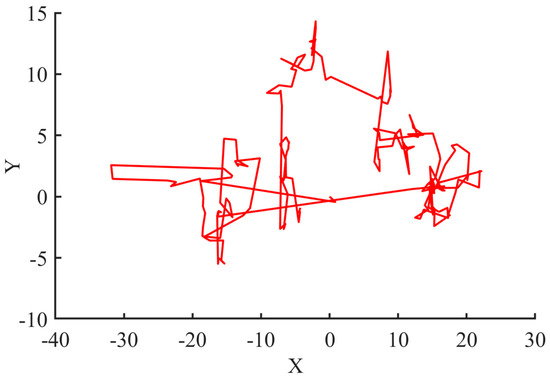
Figure 1.
2-Dimensional Levy random walk along X and Y axis.
These improvisations greatly reduce the complexity of the algorithm. In the original RSA, Equations (4) and (5) are highly complex and increase the time complexity of the algorithm. However, with the above-mentioned adaptations, we can exclude these equations from the algorithm. This means that the proposed IRSA algorithms do not have to compute these equations, which results in an almost 3-to-4-fold reduction in time complexity.
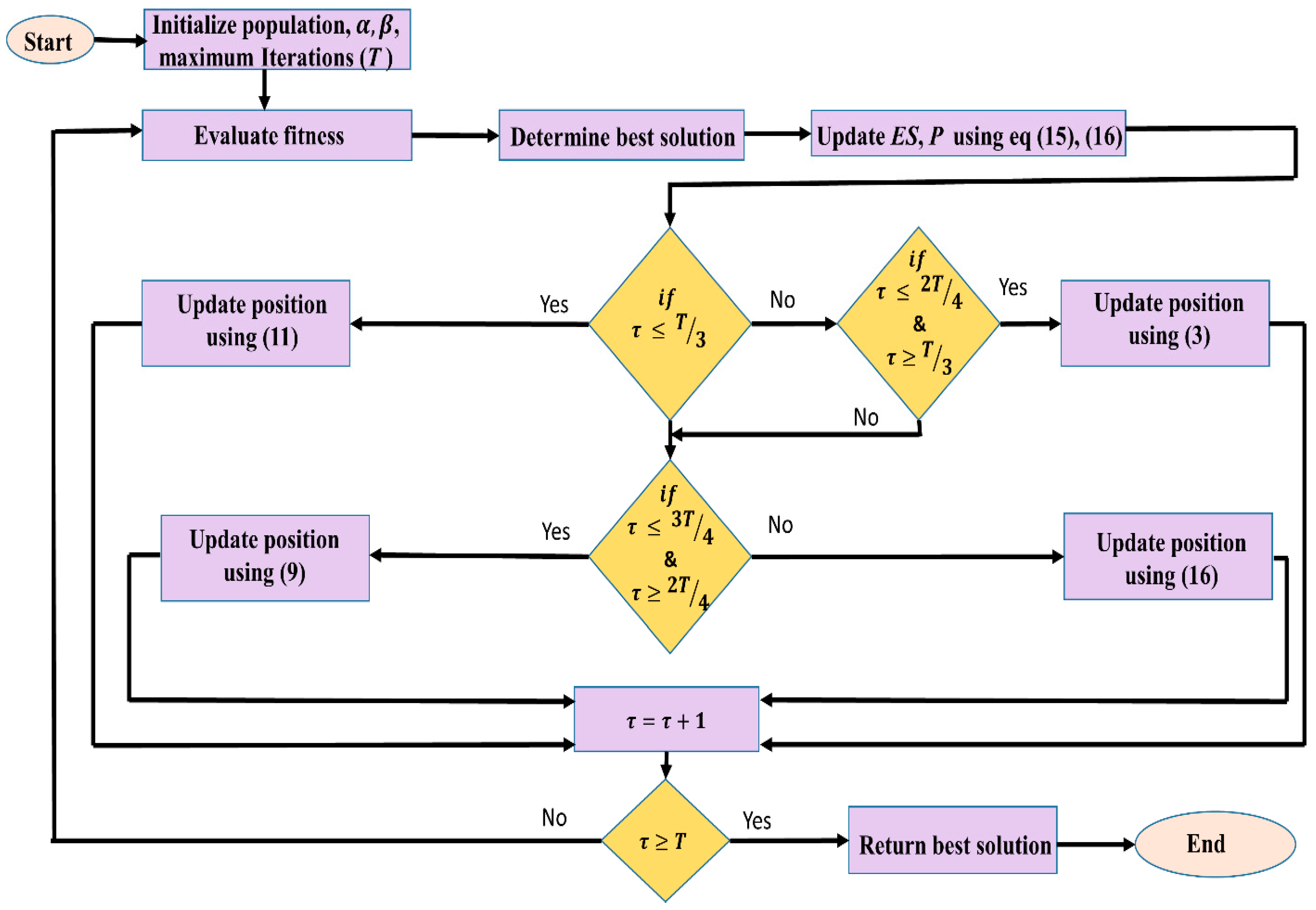
Improved global exploration, high efficiency, high convergence speed, and low time complexity are the improvements observed in the proposed technique. Taken together, the pseudocode and flowchart of the IRSA are shown in Algorithm 1 and Figure 2.
| Algorithm 1 Pseudocode of IRSA |
| Initialize random population x Initialize iteration counter= 0, maximum iteration T, alpha, beta while< T Evaluate fitness of potential candidates Determines the best solution Update Es,using Equations (6) and (7) for j = 1: p for k = 1: n If Solve using Equation (11) else if Solve using Equation (3) else if Solve using Equation (9) else Solve using Equation (16) end if end for end for t = t + 1 end while Return best solution |
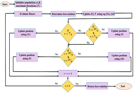
Figure 2.
Flow chart of IRSA.
3. Experimental Verification Using Benchmark Test Functions
In this section, the improved reptile search algorithm (IRSA) was tested using 23 standard benchmark functions [46]. These functions were unimodal, multimodal, and fixed-dimension minimization problems. The specifications of the test functions are provided in Table A1, Table A2 and Table A3. For further verification, the IRSA results were compared with the RSA algorithm and also with other classical and state-of-the-art metaheuristic techniques, like barnacle mating optimizer (BMO) [47], particle swarm optimization (PSO) [48], grey wolf optimizer (GWO) [49], arithmetic optimization algorithm (AOA) [50], and dynamic group-based cooperative optimization algorithm (DGCO) [51]. The numbers of iterations taken were 500 and 350, with a fixed population size of 50. For IRSA, 𝛼 and 𝛽 were set to 0.1. Furthermore, statistical analysis was performed by considering 30 runs for various performance measures like best, worse, and average values and standard deviation (STD). Lastly, time complexity analysis was performed on CEC-2019 test functions. The simulations were performed using a desktop computer Core i5 with 12 GB RAM. The software used for the simulation was MATLAB (R2018a).
3.1. Qualitative Analysis
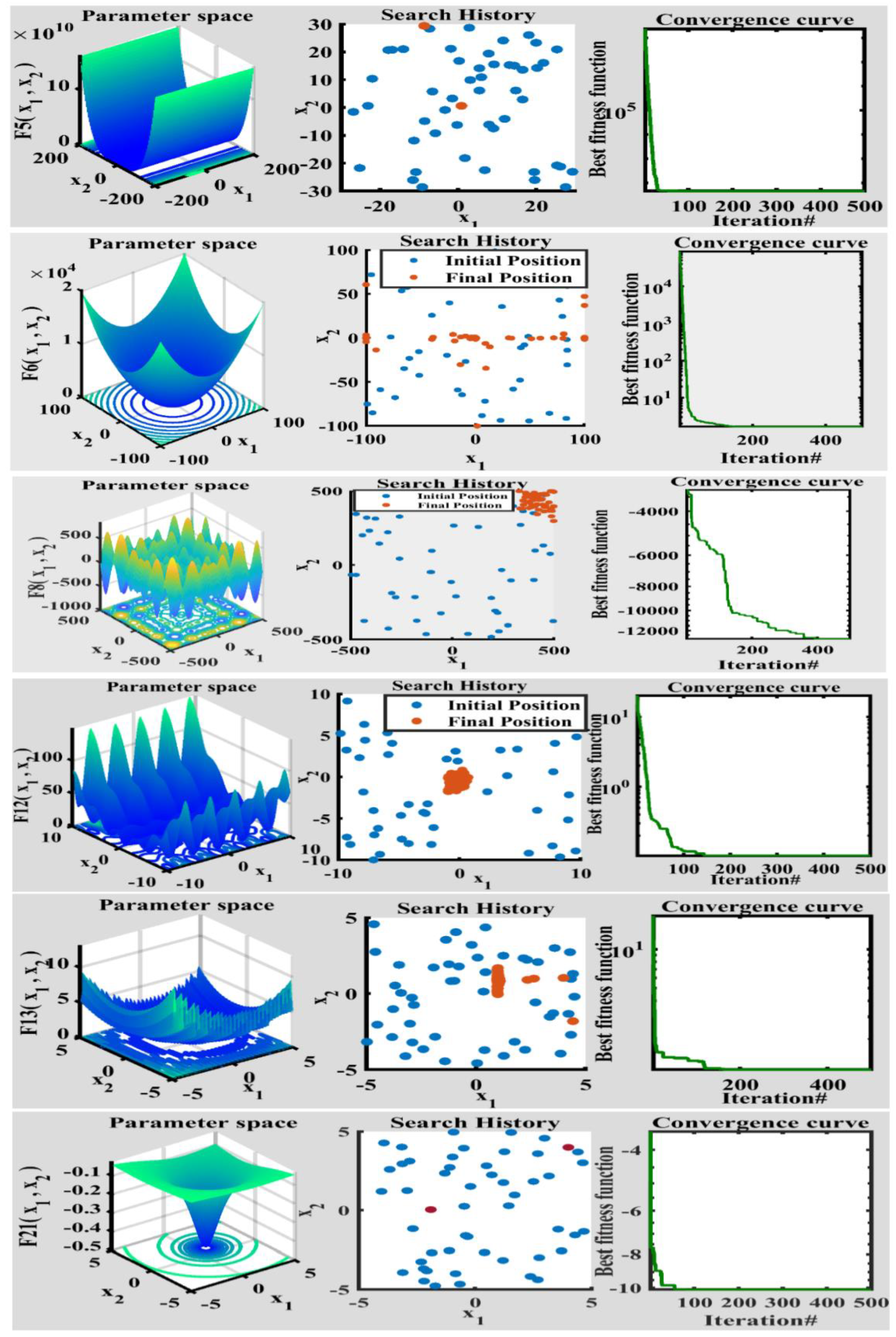
Figure 3 gives an indication of different qualitative measures used to evaluate the convergence of the RSA. The first column of each figure indicates the shape of the test functions in two dimensions to depict the topographic anatomy. The second column shows the search history, which depicts the exploration and exploitation behavior of the algorithm. The convergence curve of unimodal functions was fluid and continuous, while for multimodal functions, the curve improved in steps as they were more complex functions. It is clearly visible that the performance of the IRSA in finding an optimum solution improved significantly with an increase in the number of iterations.
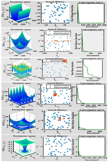
Figure 3.
Qualitative results for unimodal, multimodal, and fixed-dimension functions.
3.2. Comparative Analysis
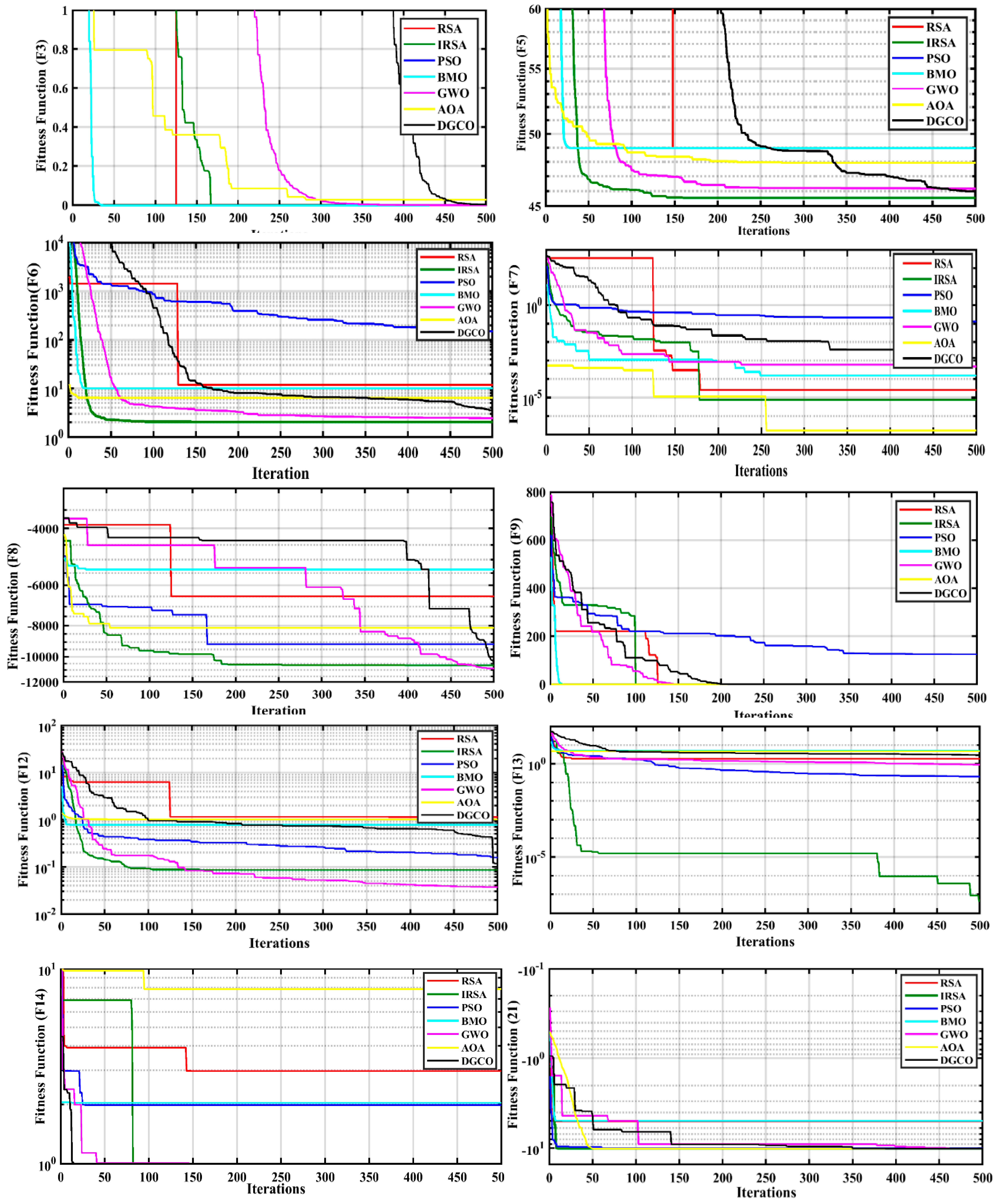
Table 1 and Table 2 show the comparative analysis between the IRSA and other MH algorithms for unimodal, multimodal, and fixed-dimension functions. For unimodal and multimodal functions, each algorithm was evaluated considering population size and iterations of 50 and 500, respectively. For statistical analysis, each algorithm ran 30 times to compute the best value, average value, worst value, and standard deviations [52]. The IRSA showed a great ability to find the optimum value on 16 out of 23 test functions, which represented nearly 70%, and it ranked second among five other test functions. The convergence curves are depicted in Figure 4. These results demonstrate the positive effects of the improvisations in the form of improved global convergence, enhanced optimization accuracy, and increased stability.

Table 1.
Results for unimodal and multimodal functions for 50 dimensions, 500 iterations.

Table 2.
Results for fixed-dimension functions considering 500 iterations.
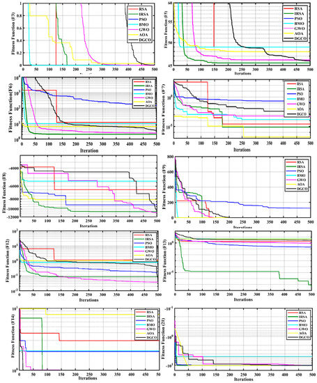
Figure 4.
Convergence curves for F1–F23.
Table 3 delineates the performance of the IRSA and other MH techniques at varying dimensions of 30, 100, and 500, considering 300 iterations. From the table, it can be observed that the IRSA provides the best results on 33 out of a total of 39 test evaluations, which represented nearly 84%, and it ranks second of five other evaluations. These results clearly demonstrate the effectiveness of the proposed algorithm in solving high-dimensional complex optimization problems.

Table 3.
Results for unimodal and multimodal functions for 30, 100, and 500 dimensions, 300 iterations.
3.3. Time Complexity Analysis
Time complexity usually depends on the initialization process, the number of iterations, and the solution update mechanism. In this section, we performed a time complexity analysis of the IRSA to determine the effect of improvisations on the computational time of the algorithm. For this purpose, we used standard benchmark test functions called CEC-2019. Table A4 delineates the specifications of these functions. The following equation is used to determine the complexity of the algorithm [53,54].
where is the computational time of a specific mathematical algorithm. was calculated to be 0.09 s; is the computational time of a CEC-2019 test function for 15,000 iterations; is the mean computational time of the MH technique used to solve CEC-2019 test functions for 10 runs considering 15,000 iterations
These computations were performed using a desktop computer Core i5 with 12 GB RAM considering a population size of 10. Table 4 and Table 5 describe the result of the analysis. The tabular results clearly show that the improvisations greatly reduce the complexity of the RSA algorithm.

Table 4.
calculation for various metaheuristic algorithms.

Table 5.
calculation for various metaheuristic algorithms.
4. IRSA for Neural Network Training
4.1. Multi-Layer Perceptron Neural Network (MLPNN)
Multi-Layer Perceptron Neural Network (MLPNN) implementing backpropagation is one of the most widely used neural network models. In MLPNN, the input layer acts as a receiver and provides the received information to the first hidden layer by passing through weights and bias, as shown in Figure 5. The information is then processed by one or multiple hidden layers and is provided to the output layer. The job of the output layers is to provide results by combining all the processed information. The activation signal for each neuron present in the hidden layer is:
where weight coefficient matrix between input, and hidden layer neurons and can be written as:
Assuming the input layer has neurons, the input vector can be written as:
If the hidden layer has neurons, then the activation signal vector can be written as:
These activation signals are applied to the neuron of the hidden layer. Based on the type of activation function, the active neuron will generate a decision signal :
For the sigmoid function, the decision signal can be calculated as:
Once decision signals for each neuron in the hidden layers are determined, these signals are multiplied with the output weight coefficient matrix to generate an estimated output as represented by the equation:
The purpose of training the MLP neural network is to find the best weight and biases to maximize classification accuracy.
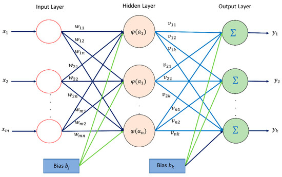
Figure 5.
MLP Neural Network.
Figure 5.
MLP Neural Network.

4.2. Radial Basis Function Neural Network (RBFNN)
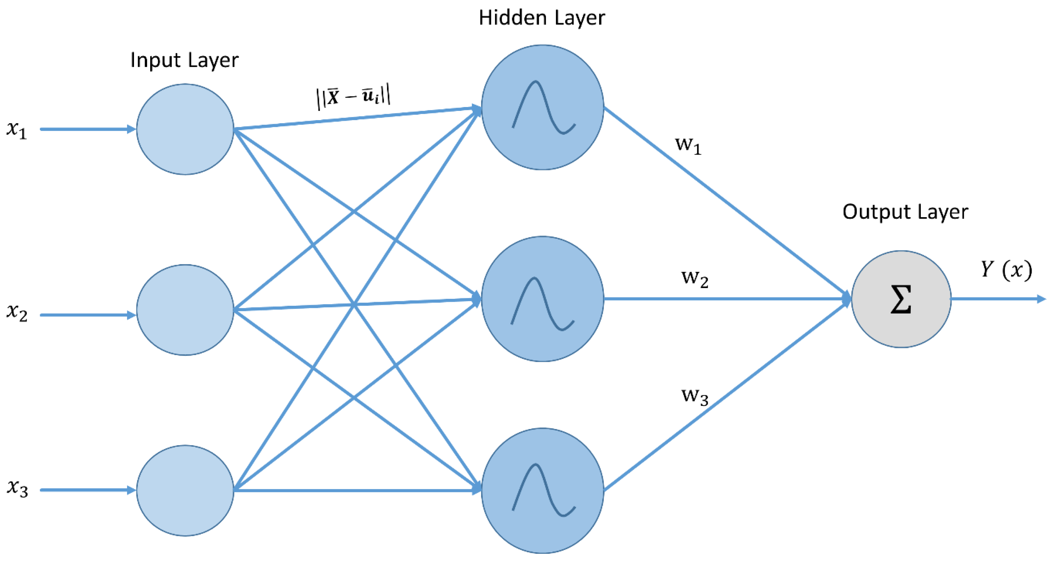
Radial Basis Function Neural Network is a three-layered universal approximator. The input layer serves as a means to connect with the environment. No computation is performed at this layer. The hidden layer consists of neurons and performs a non-linear transformation using a radial basis function. Essentially, the hidden layer transforms the pattern into higher dimensional space to make it linearly separable. The value of the ith hidden layer neuron can be written as follows:
where is the input vector, is the ith neuron’s prototype vector, is the ith neuron’s bandwidth, and is the ith neuron’s output.
The output layer performs different linear computations, which is a combination of the input and weight vector. These computations can be represented mathematically as:
where is the weight connection, is the ith neuron’s output from the hidden layer, and is the prediction result. The structure of the RBFNN is shown in Figure 6.
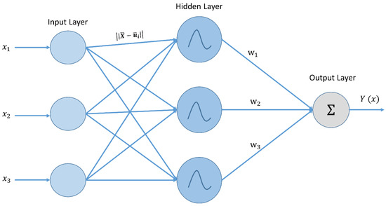
Figure 6.
Radial Basis Function Neural Network.
4.3. Training of MLPNN and RBFNN Using the Proposed IRSA
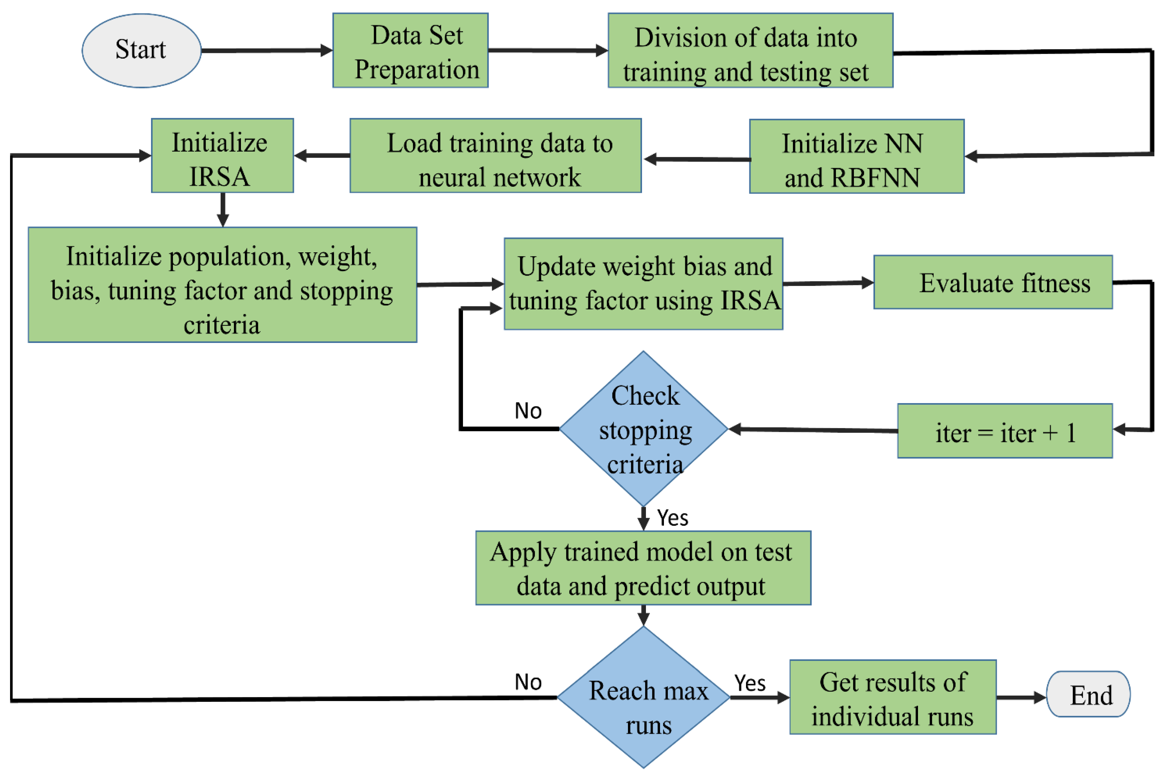
The training of parameters, such as weight and biases for MLPNN and the smoothing parameter (σ) for RBFNN, is a highly complex optimization problem. Inefficient training of these parameters results in low classification and prediction accuracy. Usually, gradient-based methods are used to train neural networks. However, these classical methods are highly dependent on initial solutions and may trap in the local minima resulting in performance degradation. Therefore, to minimize the prediction errors, the IRSA was used to determine weight, biases, and σ. Figure 7 shows the flowchart for the proposed IRSANN algorithm.
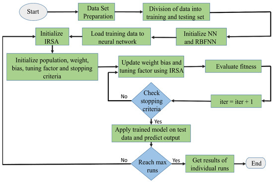
Figure 7.
Flow chart of IRSANN algorithm.
5. IRSA for Solving Classification Problems
In order to evaluate the performance of the IRSA, eight datasets obtained from [55,56] were used. Table 6 gives a brief description of the datasets. Each dataset was divided into a training set and a testing set. Almost 67% of the data was used for training the ANN, and the remaining 33% was used for testing. Sigmoid was used as an activation function for the hidden layers. Normalized mean squared error, as described by Equation (27), was used as a cost function.
where and are the true and predicted values. represents the mean of true value. N represents the total number of data samples. As there is no fixed rule to select the number of neurons, we selected neurons based on the formula [37]:
where represents the number of input features, and h shows the number of selected neurons.

Table 6.
Description of used dataset.
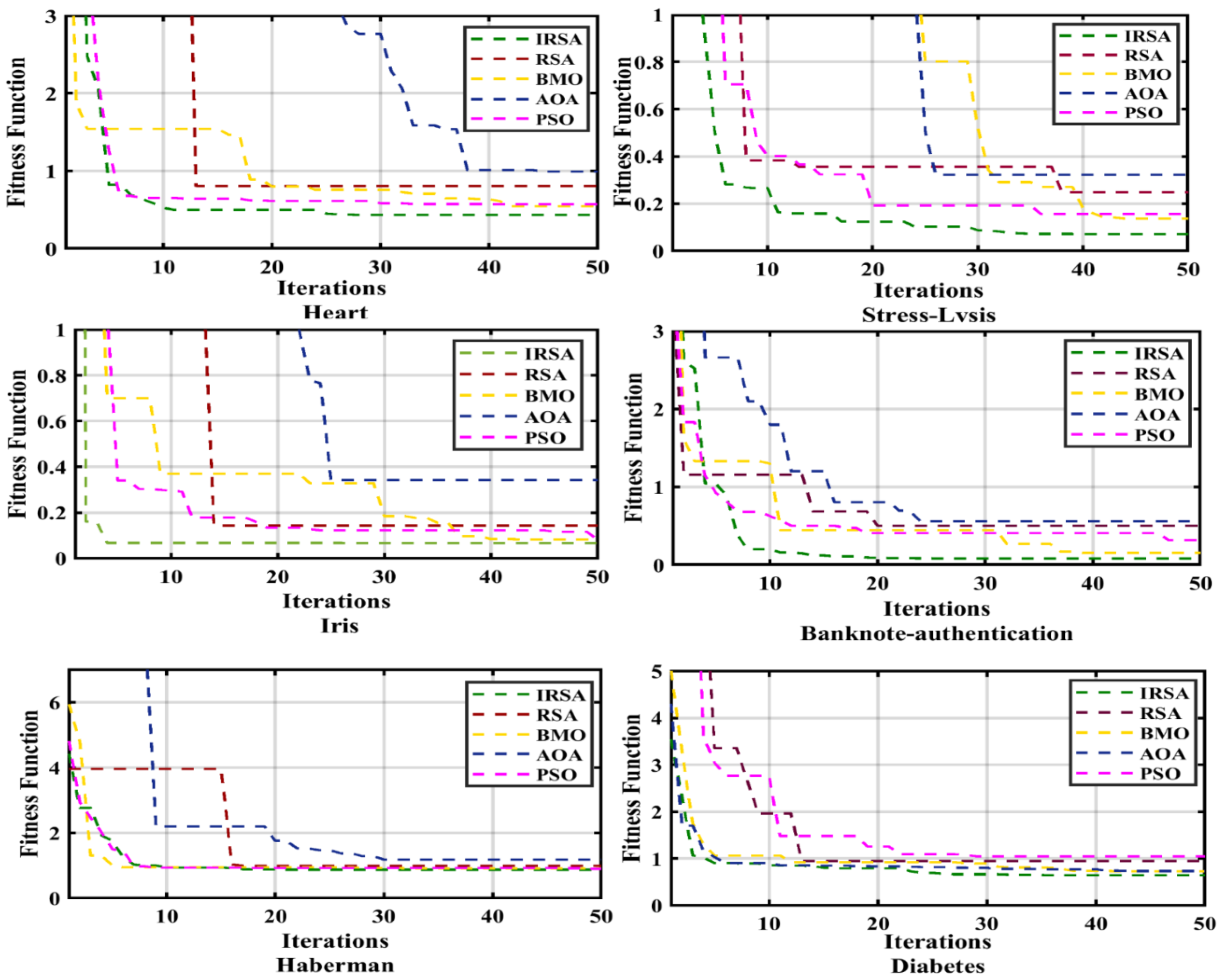
After training the MLP network, different convergence curves for IRSA, RSA, BMO, AOA, and PSO are displayed in Figure 8. The convergence of IRSA is at par with all the other metaheuristic algorithms. On the other hand, the convergence of the classical RSA was average. The accuracy while using the IRSA algorithm was better than the accuracy of other algorithms. The IRSA provided the best results for most of the datasets. Additionally, the low standard deviation of the IRSA was an indication of its strength and stability. The results in Table 7 clearly show that the accuracy of the proposed method is higher than the other four classifiers. Table 8 shows the performance of the comparative techniques in testing the dataset, and Table 9 shows the cost function comparison of all the techniques with best, average, and STD values.
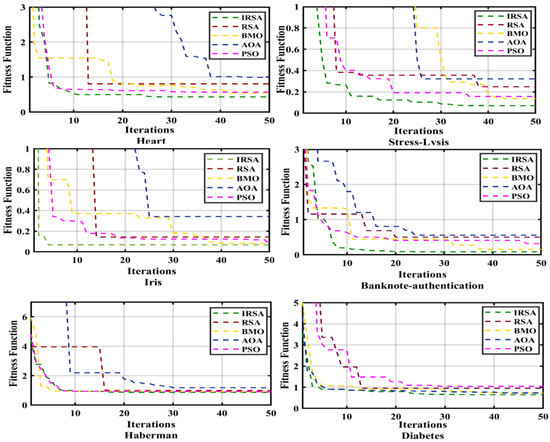
Figure 8.
Convergence curves for classification.

Table 7.
Training accuracy.

Table 8.
Testing accuracy.

Table 9.
Cost evaluation of classification dataset.
Statistical Indicators for Classification
Precision, recall, and F1 score are the parameters used to evaluate the performance of the different techniques used in this paper. Precision and recall are defined in (29) and (30) respectively:
where TP (true positive), FP (False Positive), and FN (False Negative) are determined by computing the confusion matrix. The ideal value for precision and recall is one. The F1 score can be defined as:
Table 10 represents the statistical results for the eight selected datasets. The precision, Recall, and of the proposed method were higher for six out of the eight datasets. Considering all the parameters mentioned above, we can conclude that the proposed IRSANN method provides optimum results and outperforms all other comparable MH techniques.

Table 10.
Statistical measures for classification.
6. IRSA for Solving the Regression Problems
Wind and solar energy are amongst the most promising renewable energy sources. However, wind and solar energy production are highly dependent on stochastic weather conditions. This uncertainty makes it challenging to integrate these renewable energy resources with the grid. Accurate energy prediction results in economical market operations, reliable operation planning, and efficient generation scheduling [57]. This demands highly efficient forecasting of wind and solar energy. Therefore, the IRSA is proposed to train a radial basis neural network (RBFNN) for short-term wind and solar power prediction. Normalized mean squared error, as described by equation (27), was used as a cost function. Almost 67% of the data was used for training the ANN, and the remaining 33% was used for testing.
6.1. Wind Power Prediction
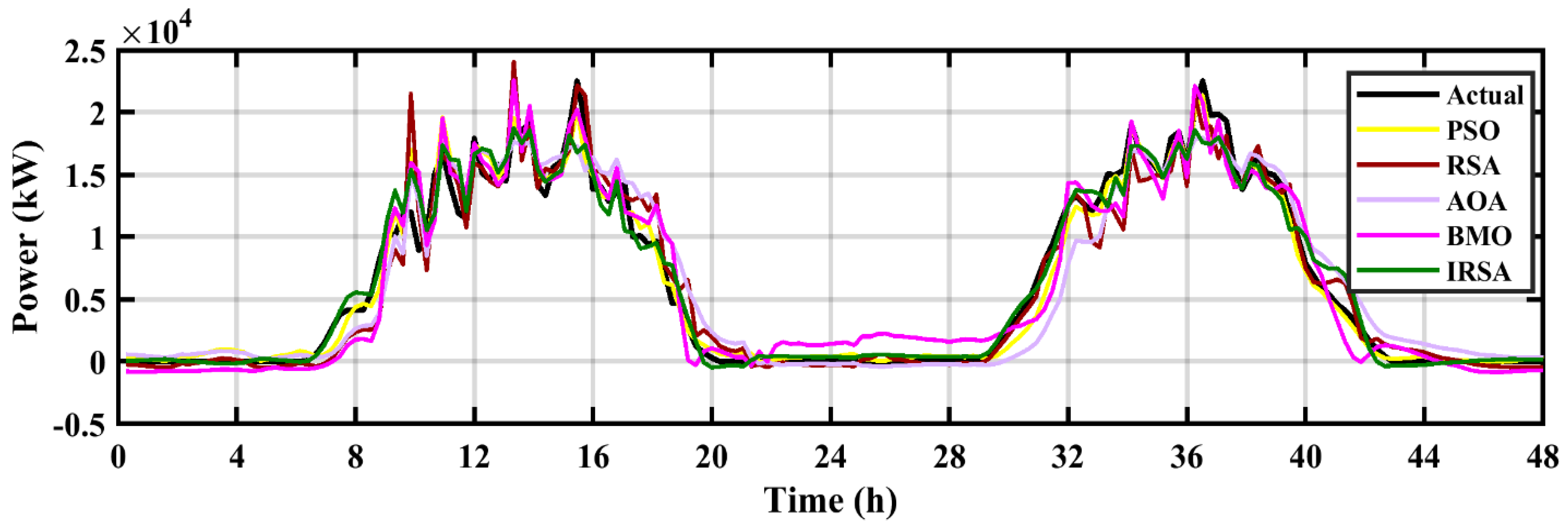
For wind power prediction, SCADA systems were used to record the wind speed, wind direction, and power generated by the wind turbine [58,59]. The measurements were taken at 10-min intervals. Figure 8 and Figure 9 show examples of the 48 h-ahead power predictions obtained by the proposed IRSA for both winter and summer seasons. A comparison between true wind power and predicted wind power by all five techniques for the winter and summer seasons is also depicted in Figure 9 and Figure 10. Simulation results clearly indicate the superior prediction capabilities of the proposed technique for both winter and the highly uncertain summer season.

Figure 9.
Wind Prediction (Winter).

Figure 10.
Wind Prediction (Summer).
6.2. Solar Power Prediction
The data set used for solar power prediction is available at [60]. The data consisted of two files. The first file contained dc and ac power generation data, and the second file contained sensor readings of ambient temperature, module temperature, and irradiance [61]. For this work, both files were combined using MATLAB code to create a dataset for solar power prediction. The readings were taken at a time interval of 15 min. The input features included ambient temperature, module temperature, and irradiance, while the output feature was the ac power. Figure 11 shows an example of the 48 h-ahead power predictions obtained by using various MH techniques. Simulation results clearly indicate the superior prediction capabilities of the proposed technique.
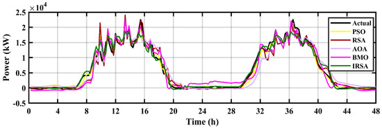
Figure 11.
Solar Power Prediction.
6.3. Statistical Indicators for Regression
In order to compare the predictive capabilities of the selected models, we used several statistical measures, such as root mean square error (RMSE), relative error (RE), and the coefficient of determination () [38]. These indicators are described by the following equations:
where and are the true and predicted values, respectively. is the mean of the value, and n represents the total number of data samples.
The small values of RMSE and RE and the higher values of give clear indications of the improved accuracy of the proposed model. These values are represented in Table 11. According to this table, the IRSA-RBFNN provides the highest values of and lowest values of RMSE for both wind and solar prediction, proving that the performance of IRSA is best when compared to other prediction models. The PSO-RBFNN model provides a slightly lower prediction efficiency. BMO-RBFN and RSA-RBFN are ranked third and fourth in terms of prediction performance [62,63].

Table 11.
Statistical evaluation for wind and solar prediction.
7. Conclusions
The main work of this paper was based on the refinement of the biologically inspired reptile search algorithm (RSA). The main objective was to enhance the exploration phase so that local minima convergence could be avoided. This was achieved by including a sine operator, which avoids local minima trapping by conducting a full-scale search of the solution space. Furthermore, the Levy flight with small steps was introduced to enhance exploitations. These improvisations enhanced not only the performance but also the results via a 3 to 4-fold reduction in the time complexity of the algorithm. The proposed improved reptile search algorithm (IRSA) was tested using various unimodal, multimodal, and fixed-dimension test functions. Finally, as an extensive application, we applied this algorithm to solving real-world classification and regression problems. The model successfully tackled the classification and regression tasks. Statistical, qualitative, quantitative, and computational complexity tests were performed to validate the effectiveness of the proposed improvisations. Based on the results, we can positively conclude that the proposed improvisations are effective in enhancing the performance of the RSA algorithm.
In the future, the IRSA could be explored to train various types of neural networks. Furthermore, applying the IRSA to solve various optimization problems in different domains (i.e., feature selection, maximum power point tracking (MPPT), smart grids, image processing, power control, robotics, etc.) would be a valuable contribution.
Author Contributions
Conceptualization, methodology, software, M.K.K.; validation, formal analysis, M.H.Z.; investigation, resources, S.R.; data curation, visualization, M.M. and S.K.R.M.; supervision, project administration, funding acquisition, F.S. All authors have read and agreed to the published version of the manuscript.
Funding
This research was funded by the Top Research Centre Mechatronics (TRCM), University of Agder (UiA), Norway, https://www.uia.no/en/research/priority-research-centres/top-researchcentre-mechatronics-trcm (accessed on 15 December 2022).
Institutional Review Board Statement
Not Applicable.
Informed Consent Statement
Not Applicable.
Data Availability Statement
The datasets generated during and/or analyzed during the current study are available from the corresponding author on reasonable request.
Conflicts of Interest
The authors declare no conflict of interest.
Appendix A

Table A1.
Utilized Unimodal Test Functions.
Table A1.
Utilized Unimodal Test Functions.
| Function Description | Dim | Range | |
|---|---|---|---|
| 500, 100, 50, 30 | [−100, 100] | 0 | |
| 500, 100, 50, 30 | [−10, 10] | 0 | |
| 500, 100, 50, 30 | [−100, 100] | 0 | |
| 500, 100, 50, 30 | [−100, 100] | 0 | |
| 500, 100, 50, 30 | [−30, 30] | 0 | |
| 500, 100, 50, 30 | [−100, 100] | 0 | |
| 500, 100, 50, 30 | [−1.28, 1.28] | 0 |

Table A2.
Utilized Multimodal Test Functions.
Table A2.
Utilized Multimodal Test Functions.
| Function Description | Dim | Range | |
|---|---|---|---|
| 500, 100, 50, 30 | [−100, 100] | −418.980 × Dim | |
| 500, 100, 50, 30 | [−10, 10] | 0 | |
| 500, 100, 50, 30 | [−100, 100] | 0 | |
| 500, 100, 50, 30 | [−100, 100] | 0 | |
here, , | 500, 100, 50, 30 | [−30, 30] | 0 |
| 500, 100, 50, 30 | [−100, 100] | 0 |

Table A3.
Utilized Fixed Dimension Test Functions.
Table A3.
Utilized Fixed Dimension Test Functions.
| Function Description | Dim | Range | |
|---|---|---|---|
| 2 | [−65, 65] | 0.998 | |
| 4 | [−1, 1] | 0 | |
| 2 | [−5, 5] | −1.0316 | |
| 2 | [−4, 4] | 0.398 | |
| 2 | [−5, 5] | 3 | |
| 3 | [−5, 5] | −3.86 | |
| 6 | [−5, 5] | −1.170 | |
| 4 | [−5, 5] | −10.153 | |
| 4 | [−5, 5] | −10.4028 | |
| 4 | [−1, 1] | −10.536 |

Table A4.
Utilized CEC 2019 Test Functions.
Table A4.
Utilized CEC 2019 Test Functions.
| Function | Description | Range | Dim | |
|---|---|---|---|---|
| CEC-1 | Storn’s Chebyshev polynomial fitting problem | 1 | [−8192, 8192] | 9 |
| CEC-2 | Inverse Hilbert matrix problem | 1 | [−16,384, 16,384] | 16 |
| CEC-3 | Lennard–Jones minimum energy cluster | 1 | [−4, 4] | 18 |
| CEC-4 | Rastrigin function | 1 | [−100, 100] | 10 |
| CEC-5 | Grienwank function | 1 | [−100, 100] | 10 |
| CEC-6 | Weierstrass function | 1 | [−100, 100] | 10 |
| CEC-7 | Modified Schwefel function | 1 | [−100, 100] | 10 |
| CEC-8 | Expanded Schaffer function | 1 | [−100, 100] | 10 |
| CEC-9 | Happy CAT function | 1 | [−100, 100] | 10 |
References
- Chong, H.Y.; Yap, H.J.; Tan, S.C.; Yap, K.S.; Wong, S.Y. Advances of metaheuristic algorithms in training neural networks for industrial applications. Soft Comput. 2021, 25, 11209–11233. [Google Scholar] [CrossRef]
- Osaba, E.; Villar-Rodriguez, E.; Del Ser, J.; Nebro, A.J.; Molina, D.; LaTorre, A.; Suganthan, P.N.; Coello, C.A.C.; Herrera, F. A Tutorial On the design, experimentation and application of metaheuristic algorithms to real-World optimization problems. Swarm Evol. Comput. 2021, 64, 100888. [Google Scholar] [CrossRef]
- Khan, M.K.; Zafar, M.H.; Mansoor, M.; Mirza, A.F.; Khan, U.A.; Khan, N.M. Green energy extraction for sustainable development: A novel MPPT technique for hybrid PV-TEG system. Sustain. Energy Technol. Assess. 2022, 53, 102388. [Google Scholar]
- Holland, J.H. Genetic algorithms. Sci. Am. 1992, 267, 66–73. [Google Scholar] [CrossRef]
- Knowles, J.; Corne, D. The Pareto archived evolution strategy: A new baseline algorithm for Pareto multiobjective optimization. In Proceedings of the 1999 Congress on Evolutionary Computation-CEC99 (Cat. No. 99TH8406), Washington, DC, USA, 6–9 July 1999. [Google Scholar]
- Mansoor, M.; Mirza, A.F.; Ling, Q. Harris hawk optimization-based MPPT control for PV Systems under Partial Shading Conditions. J. Clean. Prod. 2020, 274, 122857. [Google Scholar] [CrossRef]
- Mirjalili, S.; Gandomi, A.H.; Mirjalili, S.Z.; Saremi, S.; Faris, H.; Mirjalili, S.M. Salp Swarm Algorithm: A bio-inspired optimizer for engineering design problems. Adv. Eng. Softw. 2017, 114, 163–191. [Google Scholar] [CrossRef]
- Dorigo, M.; Birattari, M.; Stutzle, T. Ant colony optimization. IEEE Comput. Intell. Mag. 2006, 1, 28–39. [Google Scholar] [CrossRef]
- Mirjalili, S.; Lewis, A. The Whale Optimization Algorithm. Adv. Eng. Softw. 2016, 95, 51–67. [Google Scholar] [CrossRef]
- Wu, Q.; Ma, Z.; Xu, G.; Li, S.; Chen, D. A novel neural network classifier using beetle antennae search algorithm for pattern classification. IEEE Access 2019, 7, 64686–64696. [Google Scholar] [CrossRef]
- Amari, S.; Wu, S. Improving support vector machine classifiers by modifying kernel functions. Neural Netw. 1999, 12, 783–789. [Google Scholar] [CrossRef]
- Peterson, L.E. K-nearest neighbor. Scholarpedia 2009, 4, 1883. [Google Scholar] [CrossRef]
- Rish, I. An empirical study of the I Bayes classifier. In Proceedings of the IJCAI 2001 Workshop on Empirical Methods in Artificial Intelligence, Seattle, WA, USA, 8 August 2001. [Google Scholar]
- El Naqa, I.; Murphy, M. What Is Machine Learning? In Machine Learning in Radiation Oncology: Theory and Applications; El Naqa, I., Li, R., Murphy, M., Eds.; Springer International Publishing: Cham, Switzerland, 2015; pp. 3–11. [Google Scholar]
- Shanmuganathan, S. Artificial Neural Network Modelling: An Introduction. In Artificial Neural Network Modelling; Shanmuganathan, S., Samarasinghe, S., Eds.; Springer International Publishing: Cham, Switzerland, 2016; pp. 1–14. [Google Scholar]
- Sinha, A.K.; Hati, A.S.; Benbouzid, M.; Chakrabarti, P. ANN-based pattern recognition for induction motor broken rotor bar monitoring under supply frequency regulation. Machines 2021, 9, 87. [Google Scholar] [CrossRef]
- D’Addona, D.M.; Ullah, A.M.M.S.; Matarazzo, D. Tool-wear prediction and pattern-recognition using artificial neural network and DNA-based computing. J. Intell. Manuf. 2017, 28, 1285–1301. [Google Scholar] [CrossRef]
- Wu, J.; Xu, C.; Han, X.; Zhou, D.; Zhang, M.; Li, H.; Tan, K.C. Progressive Tandem Learning for Pattern Recognition with Deep Spiking Neural Networks. IEEE Trans. Pattern Anal. Mach. Intell. 2021, 44, 7824–7840. [Google Scholar] [CrossRef] [PubMed]
- Kiranyaz, S.; Avci, O.; Abdeljaber, O.; Ince, T.; Gabbouj, M.; Inman, D.J. 1D convolutional neural networks and applications: A survey. Mech. Syst. Signal Process. 2021, 151, 107398. [Google Scholar] [CrossRef]
- Poznyak, A.; Chairez, I.; Poznyak, T. A survey on artificial neural networks application for identification and control in environmental engineering: Biological and chemical systems with uncertain models. Annu. Rev. Control. 2019, 48, 250–272. [Google Scholar] [CrossRef]
- Hussain, M.; Dhimish, M.; Titarenko, S.; Mather, P. Artificial neural network based photovoltaic fault detection algorithm integrating two bi-directional input parameters. Renew. Energy 2020, 155, 1272–1292. [Google Scholar] [CrossRef]
- Veerasamy, V.; Wahab, N.I.A.; Othman, M.L.; Padmanaban, S.; Sekar, K.; Ramachandran, R.; Hizam, H.; Vinayagam, A.; Islam, M.Z. LSTM Recurrent Neural Network Classifier for High Impedance Fault Detection in Solar PV Integrated Power System. IEEE Access 2021, 9, 32672–32687. [Google Scholar] [CrossRef]
- Jiang, J.; Li, W.; Wen, Z.; Bie, Y.; Schwarz, H.; Zhang, C. Series Arc Fault Detection Based on Random Forest and Deep Neural Network. IEEE Sens. J. 2021, 21, 17171–17179. [Google Scholar] [CrossRef]
- Han, F.; Jiang, J.; Ling, Q.H.; Su, B.Y. A survey on metaheuristic optimization for random single-hidden layer feedforward neural network. Neurocomputing 2019, 335, 261–273. [Google Scholar] [CrossRef]
- Spurlock, K.; Elgazzar, H. A genetic mixed-integer optimization of neural network hyper-parameters. J. Supercomput. 2022, 78, 14680–14702. [Google Scholar] [CrossRef]
- Abd Elaziz, M.; Dahou, A.; Abualigah, L.; Yu, L.; Alshinwan, M.; Khasawneh, A.M.; Lu, S. Advanced metaheuristic optimization techniques in applications of deep neural networks: A review. Neural Comput. Appl. 2021, 33, 14079–14099. [Google Scholar] [CrossRef]
- Darwish, A.; Hassanien, A.E.; Das, S. A survey of swarm and evolutionary computing approaches for deep learning. Artif. Intell. Rev. 2020, 53, 1767–1812. [Google Scholar] [CrossRef]
- Ho, Y.-C.; Pepyne, D.L. Simple explanation of the no-free-lunch theorem and its implications. J. Optim. Theory Appl. 2002, 115, 549–570. [Google Scholar] [CrossRef]
- Abualigah, L.; Abd Elaziz, M.; Sumari, P.; Geem, Z.W.; Gandomi, A.H. Reptile Search Algorithm (RSA): A nature-inspired meta-heuristic optimizer. Expert Syst. Appl. 2022, 191, 116158. [Google Scholar] [CrossRef]
- Bou-Rabee, M.; Lodi, K.A.; Ali, M.; Ansari, M.F.; Tariq, M.; Sulaiman, S.A. One-month-ahead wind speed forecasting using hybrid AI model for coastal locations. IEEE Access 2020, 8, 198482–198493. [Google Scholar] [CrossRef]
- Farayola, A.M.; Sun, Y.; Ali, A. ANN-PSO Optimization of PV systems under different weather conditions. In Proceedings of the 2018 7th International Conference on Renewable Energy Research and Applications (ICRERA), Paris, France, 14–17 October 2018; IEEE: Piscataway, NJ, USA, 2018. [Google Scholar]
- Abdolrasol, M.G.; Mohamed, R.; Hannan, M.A.; Al-Shetwi, A.Q.; Mansor, M.; Blaabjerg, F. Artificial neural network based particle swarm optimization for microgrid optimal energy scheduling. IEEE Trans. Power Electron. 2021, 36, 12151–12157. [Google Scholar] [CrossRef]
- Banadkooki, F.B.; Ehteram, M.; Ahmed, A.N.; Teo, F.Y.; Ebrahimi, M.; Fai, C.M.; Huang, Y.F.; El-Shafie, A. Suspended sediment load prediction using artificial neural network and ant lion optimization algorithm. Environ. Sci. Pollut. Res. 2020, 27, 38094–38116. [Google Scholar] [CrossRef]
- Wongsinlatam, W.; Buchitchon, S. Criminal cases forecasting model using a new intelligent hybrid artificial neural network with cuckoo search algorithm. IAENG Int. J. Comput. Sci. 2020, 47, 481–490. [Google Scholar]
- Mehrabi, P.; Honarbari, S.; Rafiei, S.; Jahandari, S.; Alizadeh Bidgoli, M. Seismic response prediction of FRC rectangular columns using intelligent fuzzy-based hybrid metaheuristic techniques. J. Ambient. Intell. Humaniz. Comput. 2021, 12, 10105–10123. [Google Scholar] [CrossRef]
- Anand, A.; Suganthi, L. Hybrid GA-PSO optimization of artificial neural network for forecasting electricity demand. Energies 2018, 11, 728. [Google Scholar] [CrossRef]
- Faris, H.; Aljarah, I.; Mirjalili, S. Improved monarch butterfly optimization for unconstrained global search and neural network training. Appl. Intell. 2018, 48, 445–464. [Google Scholar] [CrossRef]
- Zafar, M.H.; Khan, N.M.; Mansoor, M.; Mirza, A.F.; Moosavi, S.K.R.; Sanfilippo, F. Adaptive ML-based technique for renewable energy system power forecasting in hybrid PV-Wind farms power conversion systems. Energy Convers. Manag. 2022, 258, 115564. [Google Scholar] [CrossRef]
- Zhang, J.; Wang, J.S. Improved salp swarm algorithm based on levy flight and sine cosine operator. IEEE Access 2020, 8, 99740–99771. [Google Scholar] [CrossRef]
- Iacca, G.; Junior, V.C.D.S.; de Melo, V.V. An improved Jaya optimization algorithm with Lévy flight. Expert Syst. Appl. 2021, 165, 113902. [Google Scholar] [CrossRef]
- Dahou, A.; Abd Elaziz, M.; Chelloug, S.A.; Awadallah, M.A.; Al-Betar, M.A.; Al-qaness, M.A.; Forestiero, A. Intrusion Detection System for IoT Based on Deep Learning and Modified Reptile Search Algorithm. Comput. Intell. Neurosci. 2022, 2022, 6473507. [Google Scholar] [CrossRef]
- Xiong, J.; Peng, T.; Tao, Z.; Zhang, C.; Song, S.; Nazir, M.S. A dual-scale deep learning model based on ELM-BiLSTM and improved reptile search algorithm for wind power prediction. Energy 2023, 266, 126419. [Google Scholar] [CrossRef]
- Mirjalili, S. SCA: A Sine Cosine Algorithm for solving optimization problems. Knowl. Based Syst. 2016, 96, 120–133. [Google Scholar] [CrossRef]
- Chechkin, A.; Metzler, R.; Klafter, J.; Gonchar, V.Y. Introduction to the Theory Lévy Flights. In Anomalous Transport: Foundations and Applications; Wiley-VCH: Weinheim, Germany, 2008. [Google Scholar]
- Yang, X.-S.; Deb, S. Multiobjective cuckoo search for design optimization. Comput. Oper. Res. 2013, 40, 1616–1624. [Google Scholar] [CrossRef]
- Xin, Y.; Yong, L.; Guangming, L. Evolutionary programming made faster. IEEE Trans. Evol. Comput. 1999, 3, 82–102. [Google Scholar] [CrossRef]
- Sulaiman, M.H.; Mustaffa, Z.; Saari, M.M.; Daniyal, H. Barnacles mating optimizer: A new bio-inspired algorithm for solving engineering optimization problems. Eng. Appl. Artif. Intell. 2020, 87, 103330. [Google Scholar] [CrossRef]
- Kennedy, J.; Eberhart, R. Particle swarm optimization. In Proceedings of the ICNN’95—International Conference on Neural Networks, Perth, Australia, 27 November–1 December 1995. [Google Scholar]
- Mirjalili, S.; Mirjalili, S.M.; Lewis, A. Grey Wolf Optimizer. Adv. Eng. Softw. 2014, 69, 46–61. [Google Scholar] [CrossRef]
- Abualigah, L.; Diabat, A.; Mirjalili, S.; Abd Elaziz, M.; Gandomi, A.H. The Arithmetic Optimization Algorithm. Comput. Methods Appl. Mech. Eng. 2021, 376, 113609. [Google Scholar] [CrossRef]
- Fouad, M.M.; El-Desouky, A.I.; Al-Hajj, R.; El-Kenawy, E.S.M. Dynamic Group-Based Cooperative Optimization Algorithm. IEEE Access 2020, 8, 148378–148403. [Google Scholar] [CrossRef]
- Zafar, M.H.; Khan, N.M.; Moosavi, S.K.R.; Mansoor, M.; Mirza, A.F.; Akhtar, N. Artificial Neural Network (ANN) trained by a Novel Arithmetic Optimization Algorithm (AOA) for Short Term Forecasting of Wind Power. In Proceedings of the International Conference on Intelligent Technologies and Applications (INTAP), Grimstad, Norway, 11–13 October 2022; Springer: Berlin/Heidelberg, Germany, 2022; pp. 197–209. [Google Scholar]
- Liang, J.J.; Suganthan, P.N.; Chen, Q. Problem definitions and evaluation criteria for the CEC 2013 special session on real-parameter optimization. Comput. Intell. Lab. Zhengzhou Univ. Zhengzhou China Nanyang Technol. Univ. Singap. Tech. Rep. 2013, 201212, 281–295. [Google Scholar]
- Mansoor, M.; Ling, Q.; Zafar, M.H. Short Term Wind Power Prediction using Feedforward Neural Network (FNN) trained by a Novel Sine-Cosine fused Chimp Optimization Algorithm (SChoA). In Proceedings of the 2022 5th International Conference on Energy Conservation and Efficiency (ICECE), Lahore, Pakistan, 16–17 March 2022; IEEE: Piscataway, NJ, USA, 2022. [Google Scholar]
- Available online: https://archive.ics.uci.edu/ml/index.php (accessed on 17 September 2022).
- Available online: https://www.kaggle.com/datasets (accessed on 30 September 2022).
- Al-Dahidi, S.; Ayadi, O.; Alrbai, M.; Adeeb, J. Ensemble approach of optimized artificial neural networks for solar photovoltaic power prediction. IEEE Access 2019, 7, 81741–81758. [Google Scholar] [CrossRef]
- Şahin, S.; Türkeş, M. Assessing wind energy potential of Turkey via vectoral map of prevailing wind and mean wind of Turkey. Theor. Appl. Climatol. 2020, 141, 1351–1366. [Google Scholar] [CrossRef]
- Available online: https://www.kaggle.com/datasets/berkerisen/wind-turbine-scada-dataset (accessed on 13 October 2022).
- Available online: https://www.kaggle.com/datasets/anikannal/solar-power-generation-data (accessed on 10 October 2022).
- Zafar, M.H.; Khan, U.A.; Khan, N.M. Hybrid Grey Wolf Optimizer Sine Cosine Algorithm based Maximum Power Point Tracking Control of PV Systems under Uniform Irradiance and Partial Shading Condition. In Proceedings of the 2021 4th International Conference on Energy Conservation and Efficiency (ICECE), Lahore, Pakistan, 16–17 March 2021; IEEE: Piscataway, NJ, USA, 2021. [Google Scholar]
- Zafar, M.H.; Khan, N.M.; Mirza, A.F.; Mansoor, M.; Akhtar, N.; Qadir, M.U.; Khan, N.A.; Moosavi, S.K.R. A novel meta-heuristic optimization algorithm based MPPT control technique for PV systems under complex partial shading condition. Sustain. Energy Technol. Assess. 2021, 47, 101367. [Google Scholar]
- Mansoor, M.; Mirza, A.F.; Duan, S.; Zhu, J.; Yin, B.; Ling, Q. Maximum energy harvesting of centralized thermoelectric power generation systems with non-uniform temperature distribution based on novel equilibrium optimizer. Energy Convers. Manag. 2021, 246, 114694. [Google Scholar] [CrossRef]
Disclaimer/Publisher’s Note: The statements, opinions and data contained in all publications are solely those of the individual author(s) and contributor(s) and not of MDPI and/or the editor(s). MDPI and/or the editor(s) disclaim responsibility for any injury to people or property resulting from any ideas, methods, instructions or products referred to in the content. |
© 2023 by the authors. Licensee MDPI, Basel, Switzerland. This article is an open access article distributed under the terms and conditions of the Creative Commons Attribution (CC BY) license (https://creativecommons.org/licenses/by/4.0/).


